Application of Statistical Distribution Models to Predict Health Index for Condition-Based Management of Transformers

Abstract

In this study, statistical distribution model (SDM) is used to predict the health index (HI) of transformers by utilizing the condition parameters data from dissolved gas analysis (DGA), oil quality analysis (OQA), and furanic compound analysis (FCA), respectively. First, the individual condition parameters data were categorized based on transformer age from year 1 to 15. Next, the individual condition parameters data for every age were fitted while using a probability plot to find the representative distribution models. The distribution parameters were calculated based on 95% confidence level and extrapolated from year 16 to 25 through representative fitting models. The individual condition parameters data within the period were later calculated based on the estimated distribution parameters through the inverse cumulative distribution function (ICDF) of the selected distribution models. The predicted HI was then determined based on the conventional scoring method. The Chi-square test for statistical hypothesis reveals that the predicted HI for the transformer data is quite close to the calculated HI. The average percentage of absolute error is 2.7%. The HI that is predicted based on SDM yields 97.83% accuracy for the transformer data.

1. Introduction

Power transformers are among the most expensive and critical units in electrical distribution systems. Improper operational intervention could affect the power delivery, which results in substantial repair or replacement costs to the utilities. In recent years, utilities have shifted into predictive maintenance due to an advancement of data driven in maintenance program. Transformer’s condition-based management (CBM) database has been given significant attention and utilized for the development of the health index (HI) model in order to optimize the investment and ensure reliable operation.

HI is a known method that utilizes the in-service multiple condition information into an objective and single computable index to provide the inclusive health of the transformer asset. This technique helps to assess the long-term degradation level of transformer population through the condition parameters data, which may not be accessible to be diagnosed by scheduled maintenance and individual diagnostic techniques [1]. HI can be used for the management of the assets and prioritization of the investment in either capital or maintenance schemes [1]. HI concept is based on scoring, rating, and ranking methods, which considers fundamental theory, technical guidelines, and expert decisions. Most utilities employ HI for the management of transformer assets, such as Kinectrics Inc., DNV GL, Hydro-Québec, Terna, Electricity Generating Authority of Thailand, and Tenaga Nasional Berhad [2,3,4,5,6].

Common data driven approaches, such as statistical and artificial intelligence (AI) application based models, have been widely used as prediction models for condition deterioration of high voltage assets [7,8,9,10]. Predicting the HI of the transformers based on these approaches is one of many other applications. This will substantially help in the financial strategy of the utilities in asset maintenance plans. Currently, there are limited studies on the modelling of future transformers’ health degradation that is based on HI. Most of the studies focus on the prediction based on the individual condition parameters data [11,12,13,14].

Statistical approaches that are based on Markov Model (MM) [15,16] and Hidden Markov Model (HMM) [17] have been used to predict the condition states of transformer population. Previous work in [15] utilizes the transition probabilities of the transformer’s condition states that are derived from HI for a specific year interval. The other study in [16] implements a similar approach, except that the transformer’s condition states are derived from condition parameters data. A previous study in [17] utilizes HMM to predict the transformer’s condition states in a different approach as compared to MM [15,16]. Hidden state transition and emission probabilities derived from condition parameters data have been computed to predict the HI of transformers [17]. MM and HMM both do not rely heavily on historical condition parameters data. Hence, the uncertainty effect due to constraints of a long-term data record could be minimized. The methods predict either the final HI or individual condition parameters in terms of probabilities, which were later converted into HI and condition parameters data values. It is found that the accuracy levels of HI that were obtained based on these models have been satisfactory.

On the other hand, fuzzy logic [18], general regression neural network (GRNN) [19], neural-fuzzy (NF) [20], random forest [21], support vector machine (SVM) [22], principle component analysis (PCA), and analytical hierarchy process (AHP) [23], are among the available AI models that have been studied in previous works of HI. These models require extensive data to ensure a promising result in terms of prediction accuracy of the condition of the transformers.

The main motivation of this study is to introduce a simplified method in order to predict the HI of transformer population that is based on Statistical Distribution Model (SDM) utilizing the individual condition parameter data as a key approach to determine the HI. SDM is chosen, due to its simplicity and adaptability to analyze any sample size data [24]. In addition, it can also identify the independent variables (13 condition parameters) that can affect the predicted HI. Hence, further investigation can be performed on the abnormal trend of the individual condition parameters data to improve the interpretation of overall transformer’s HI. First, the representative distribution model is identified for the individual condition parameters data of transformers. Next, the SDM is implemented to the condition parameters data to determine the predicted HI of transformer population. The final part is on hypothesis testing through the Chi-square statistic to determine the best-of-fit and absolute error percentage between the predicted and computed HI.

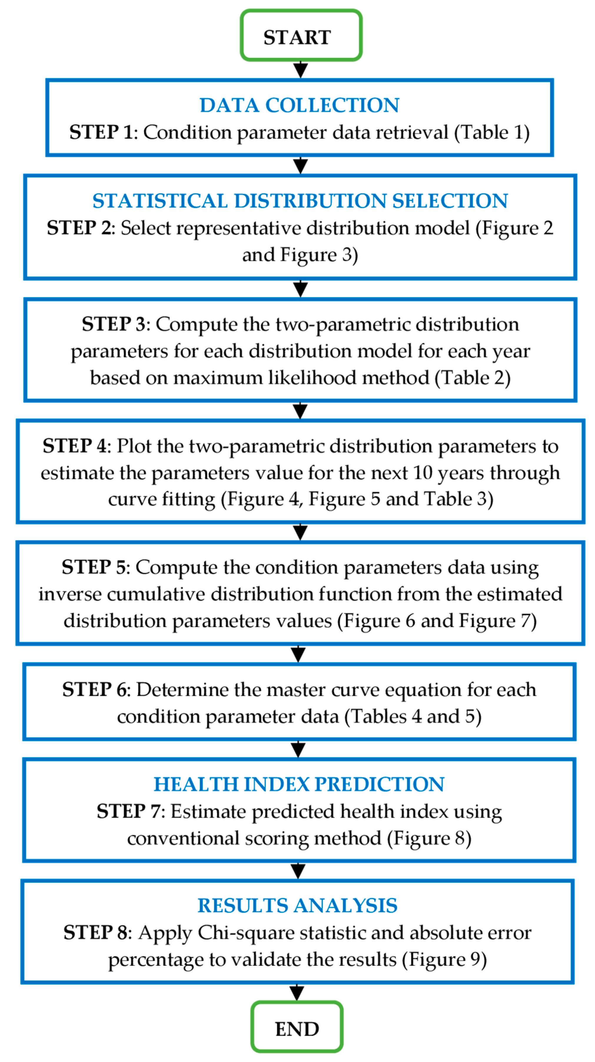
2. Transformer Health Index Estimation Model

SDM was employed in order to predict the HI of the transformer population, given the limited historical condition parameters data. Figure 1 shows the overall framework for estimating the impending transformer HI using individual condition parameters data. First, the condition parameters data from the transformer population were grouped according to age band from year 1 to 15. Next, the individual condition parameters data of transformers data for every age were fitted into the probability plot to determine the representative distribution. The distribution parameters from year 1 to 15 were then calculated. The distribution parameters were then plotted and extrapolated to determine the distribution parameters for the next 10 years. Next, the individual condition parameters data were calculated from the extrapolated distribution parameters that were based on the inverse cumulative distribution function (ICDF) of the identified distribution model. The predicted HI was then determined based on the conventional scoring approach. Finally, the predicted HI was compared with computed HI using the Chi-square test and absolute error percentage.

The HI of transformer population was modelled based on the statistical approach. The method was used to estimate the predicted HI by calibrating the prediction model based on the condition parameters data. The first condition parameters data that were considered for the input parameters were from dissolved gas analysis (DGA), which included hydrogen (H₂), methane (CH₄), acetylene (C₂H₂), ethylene (C₂H₄), ethane (C₂H₆), carbon monoxide (CO), and carbon dioxide (CO₂). The oil quality analysis (OQA) included dielectric breakdown voltage, interfacial tension, color, acidity, and water content. The furanic compound analysis (FCA) that consisted of 2-furfuraldehyde (2-FAL) was also used in the study to consider the in-service ageing of the solid insulation. It is important to note that this study does not consider any abnormal data due to the unusual operating environment, internal electrical faults, and electromagnetic interference during in-service.

In this study, two-parametric Weibull and normal distribution models were considered. Weibull distribution has been widely used for industrial applications, especially in the field of reliability engineering. It is normally used in the reliability assessment, such as the derivation of reliability indices mean time to failure (MTTF) [25], equipment’s failure rate [26,27,28], remaining useful life prediction [29,30], spare parts replacement, and maintenance/replacement strategies [31,32]. It is a versatile distribution with two critical parameters, which can also describe the characteristics of other types of distributions. The probability density function (PDF) of the Weibull distribution model was computed based on the condition data parameters and it is expressed in Equation (1) [33].

$$f\left(t\right)=\frac{\beta }{\alpha }{\left(\frac{t}{\alpha }\right)}^{\beta -1}ex{p}^{-{\left(\frac{t}{\alpha }\right)}^{\beta }}$$

(1)

where $t$ is the lifetime of the transformer, $\beta$ is the shape parameter, and $\alpha$ is the scale parameter. $\alpha$ determines the spread of the data, while $\beta$ implies the shape of the distribution, whereby it is dimensionless. Different values of the $\beta$ can affect the behavior of the distribution. For $3\le \beta \le 4$, the shape of the Weibull distribution is similar to that of a normal model. In order tso plot the probability of Weibull distribution, the condition parameters data were converted into probabilities using CDF, as shown in Equation (2) [34].

$$F\left(t\right)=\underset{0}{\overset{T}{{\displaystyle \int }}}f\left(t\right)=1-ex{p}^{-{\left(\frac{t}{\alpha }\right)}^{\beta }}$$

(2)

Normal or Gaussian distribution has wide application in describing product lifetime data [35], and it can be expressed by Equation (3) [36].

$$f\left(t\right)=\frac{1}{\sqrt{2\pi \sigma }}ex{p}^{\left[-\frac{{\left(t-\mu \right)}^2}{2{\sigma }^2}\right]}$$

(3)

in which $\mu$ is the mean of the distribution and $\sigma$ is the standard deviation. Both of the parameters are in the same unit as the variable $t$. The Normal CDF can be expressed by Equation (4) [37].

$$F\left(t\right)={{\displaystyle \int }}_o^t\frac{1}{\sqrt{2\pi \sigma }}ex{p}^{\left[-\frac{{\left(t-\mu \right)}^2}{2{\sigma }^2}\right]}dy$$

(4)

where $F\left(t\right)$ is the CDF for the standard normal distribution (with $\mu =0$ and $\sigma =1$).

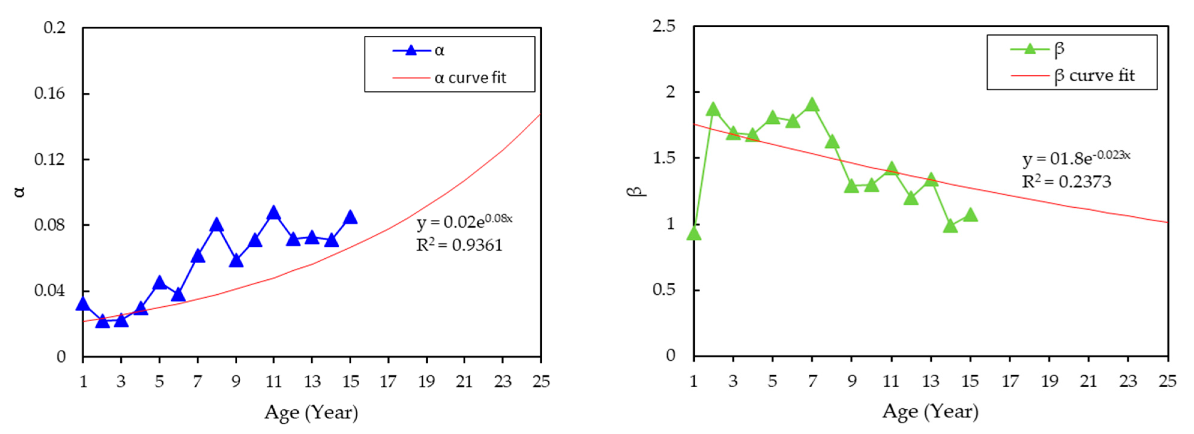
2.1. Estimations Distribution Parameters Estimation

There are several methods that can be used in order to estimate the Weibull and normal distributions parameters, such as the ordinary least square (OLS), weighted least square (WLS), maximum likelihood estimate (MLE), and method of moments (MOM) [33]. The OLS and the WLS methods are commonly used due to its simplicity [37]. The parameters estimation can be calculated by solving the simultaneous equations. The MLE and the MOM are the common methods that are used for engineering analyses, but both are computationally demanding [37]. Moreover, MLE and likelihood functions normally desire significant numbers of sample size, which develop unbiased minimum variance estimators as the sample size increases [38,39]. In this paper, the MLE method was used for estimating the population parameters of a distribution. It is because MLE is an analytic maximization procedure, which is applicable to all form of data [34]. These methods also have approximate normal distributions and sample variances that can be utilized to produce confidence bounds likelihood functions to test the models and parameters’ hypotheses.

Suppose that $x_1,x_2,\dots ,x_n$ are independent and identically distributed Weibull parameters, the random variables have probability density function $f\left(x\right)$ expressed in Equation (1), where the parameters are assumed to be unknown. The MLE method was employed to estimate the parameters $\alpha$ and $\beta$. The likelihood function of $x_1,x_2,\dots ,x_n$ can be constructed from Equation (2) and expressed in Equation (5) [40],

$$L\left(\alpha ,\beta \right)={\alpha }^n{\beta }^n{\left({\displaystyle \prod }_{i=1}^n{x}_i\right)}^{\beta -1}exp\left(-\alpha {\displaystyle \sum }_{i=1}^n{x}_i^{\beta }\right)$$

(5)

Equation (6) can be obtained by taking the natural logarithmic transformation of Equation (5).

$$lnL\left(\alpha ,\beta \right)=nln\alpha +nln\beta +\left(\beta -1\right){\displaystyle \sum }_{i=1}^{n}ln{x}_i-\alpha {\displaystyle \sum }_{i=1}^n{x}_i^{\beta }$$

(6)

Differentiating Equation (6) with respect to $\alpha$ and $\beta$, respectively, yields Equations (7) and (8).

$$\frac{\partial }{\partial \alpha }lnL\left(\alpha ,\beta \right)=\frac{n}{\alpha }-{\displaystyle \sum }_{i=1}^n{x}_i^{\beta }$$

(7)

$$\frac{\partial }{\partial \alpha }lnL\left(\alpha ,\beta \right)=\frac{n}{\beta }+{\displaystyle \sum }_{i=1}^{n}ln{x}_i-\alpha {\displaystyle \sum }_{i=1}^n{x}_i^{\beta }ln{x}_i$$

(8)

Hence, the MLE estimates $(\widehat{\alpha },\widehat{\beta })$ of $\left(\alpha ,\beta \right)$ can be estimated from the following Equations (9) and (10).

$$\frac{n}{\widehat{\alpha }}={\displaystyle \sum }_{i=1}^n{x}_i^{\widehat{\beta }}$$

(9)

$$\frac{n}{\widehat{\beta }}={\displaystyle \sum }_{i=1}^{n}ln{x}_i=\widehat{\alpha }{\displaystyle \sum }_{i=1}^n{x}_i^{\widehat{\beta }}ln{x}_i$$

(10)

or equivalently

$$\widehat{\alpha }=\frac{n}{{{\displaystyle \sum }}_i^n{x}_i^{\widehat{\beta }}}$$

(11)

$$n+\widehat{\beta }{\displaystyle \sum }_{i=1}^{n}ln{x}_i=\frac{n\widehat{\beta }{{\displaystyle \sum }}_{i=1}^n{x}_i^{\widehat{\beta }}ln{x}_i}{{{\displaystyle \sum }}_{i=1}^n{x}_i^{\widehat{\beta }}}$$

(12)

Equations (11) and (12) can be numerically solved for $\widehat{\beta }$ and $\widehat{\alpha }$. Similarly, for normal distribution, the parameters $\mu$ and $\sigma$ were estimated using the MLE. The likelihood function of $x_1,x_2,\dots ,x_n$ can be constructed from Equation (4) and it is expressed in Equation (13).

$$L\left(\mu ,\sigma \right)={\displaystyle \prod }_{i=1}^n\frac{1}{\sigma \sqrt{2\pi }}exp\left(-\frac{1}{2}{\left[\frac{x_i-\mu }{\sigma }\right]}^2\right)$$

(13)

From Equation (13), the log-likelihood can be expressed based on (14).

$$l\left(\mu ,\sigma \right)=-nlog\sigma -\frac{n}{2}log2\pi -\frac{1}{2{\sigma }^2}{\displaystyle \sum }_{i=1}^n{\left(x_i-\mu \right)}^2$$

(14)

Differentiating Equation (14) with respect to $\mu$ and $\sigma$, respectively, yields Equations (15) and (16).

$$\frac{\partial l}{\partial \mu }=\frac{1}{{\sigma }^2}{\displaystyle \sum }_{i=1}^n\left(x_i-\mu \right)$$

(15)

$$\frac{\partial l}{\partial \sigma }=-\frac{n}{\sigma }+{\sigma }^{-3}{\displaystyle \sum }_{i=1}^n{\left(x_i-\mu \right)}^2$$

(16)

Equating Equation (15) to zero, the MLE $(\widehat{\mu },\widehat{\sigma })$ of $\left(\mu ,\sigma \right)$ solutions are expressed in Equation (17).

$$\widehat{\mu }=\overline{X}$$

(17)

Equating Equation (16) to zero and substituting the MLE for $\mu$ with Equation (17), Equation (18) represents the MLE for $\sigma$.

$$\widehat{\sigma }=\sqrt{\frac{1}{n}{\displaystyle \sum }_{i=1}^n{\left(x_i-\overline{X}\right)}^2}$$

(18)

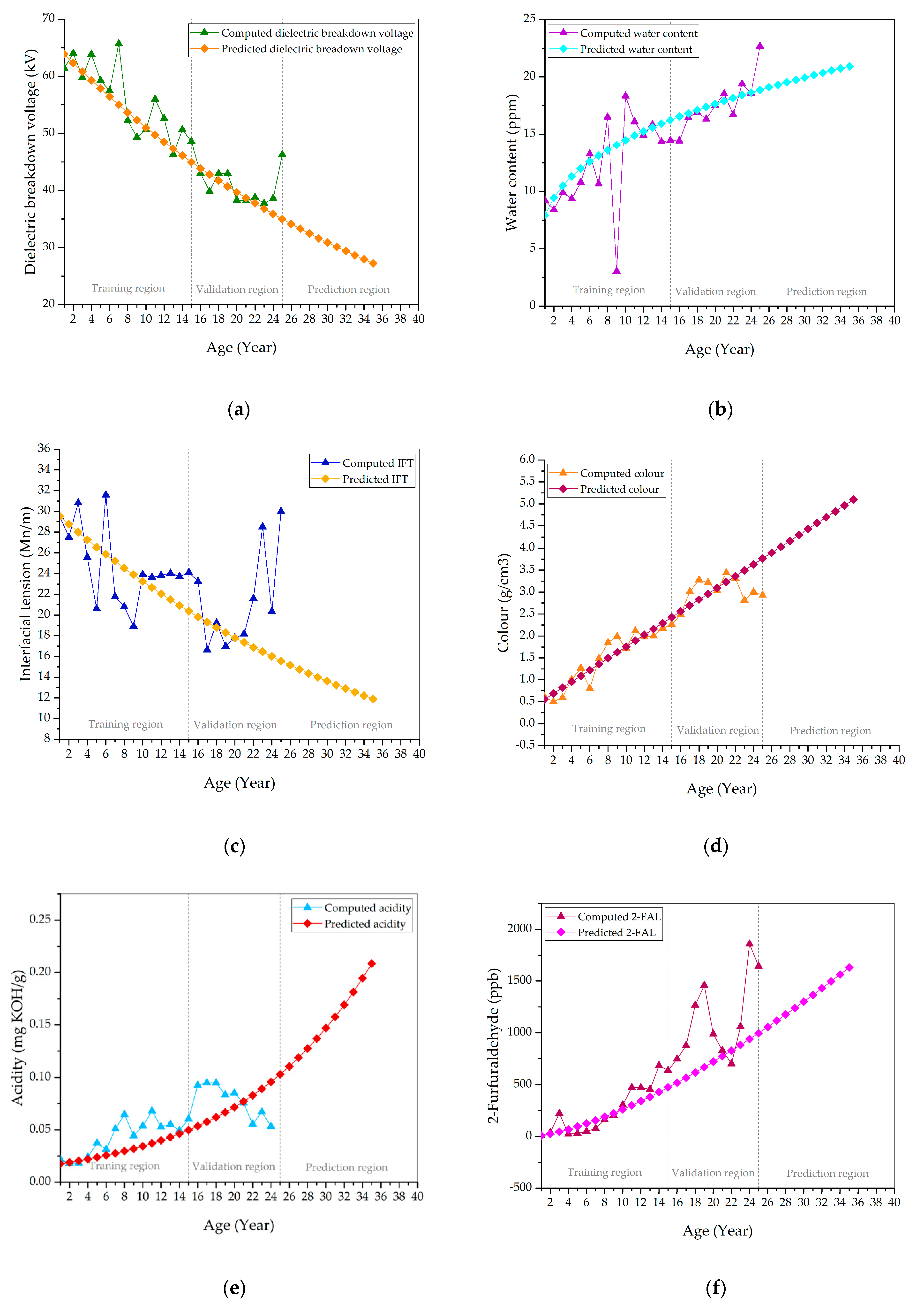
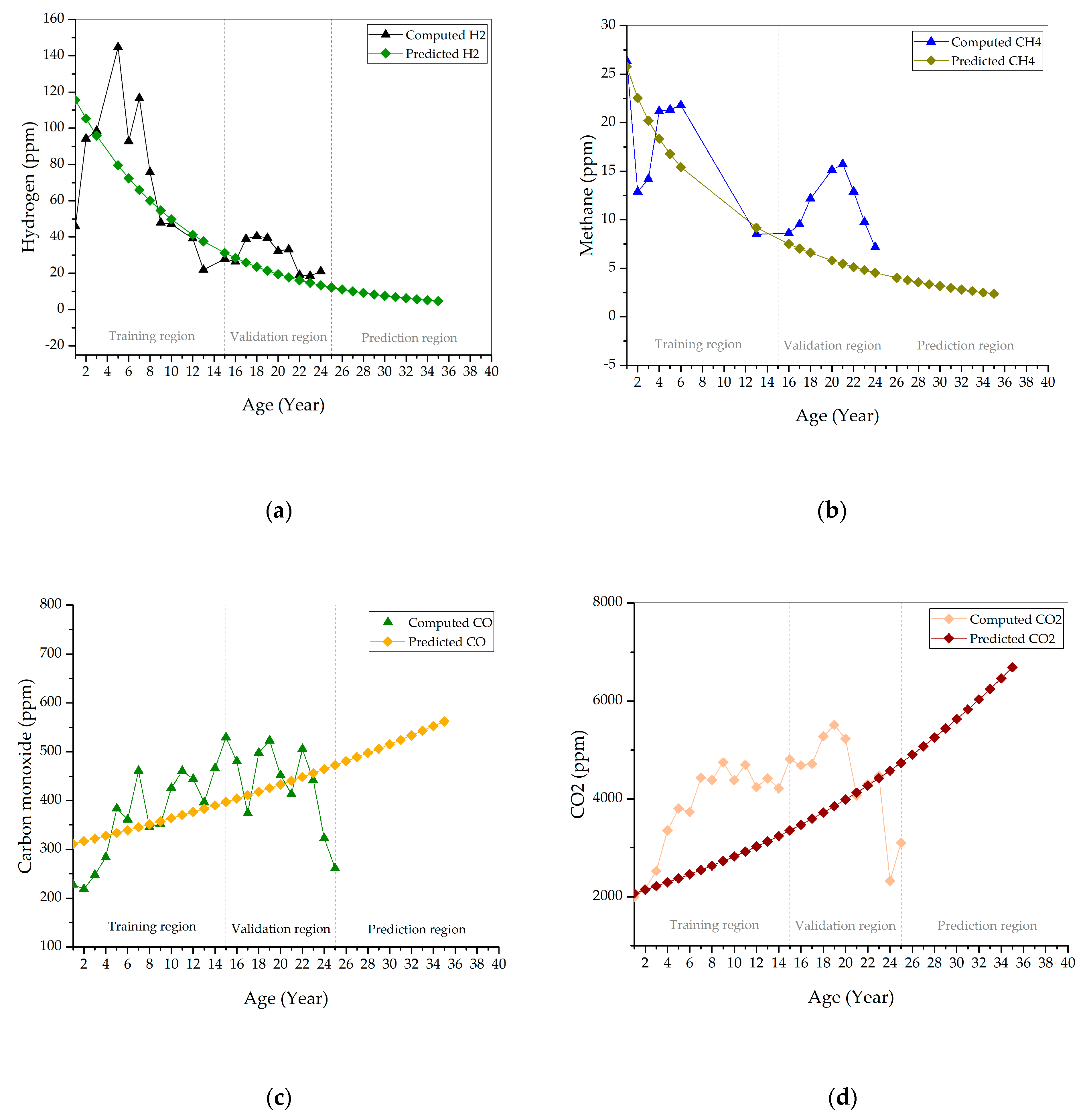
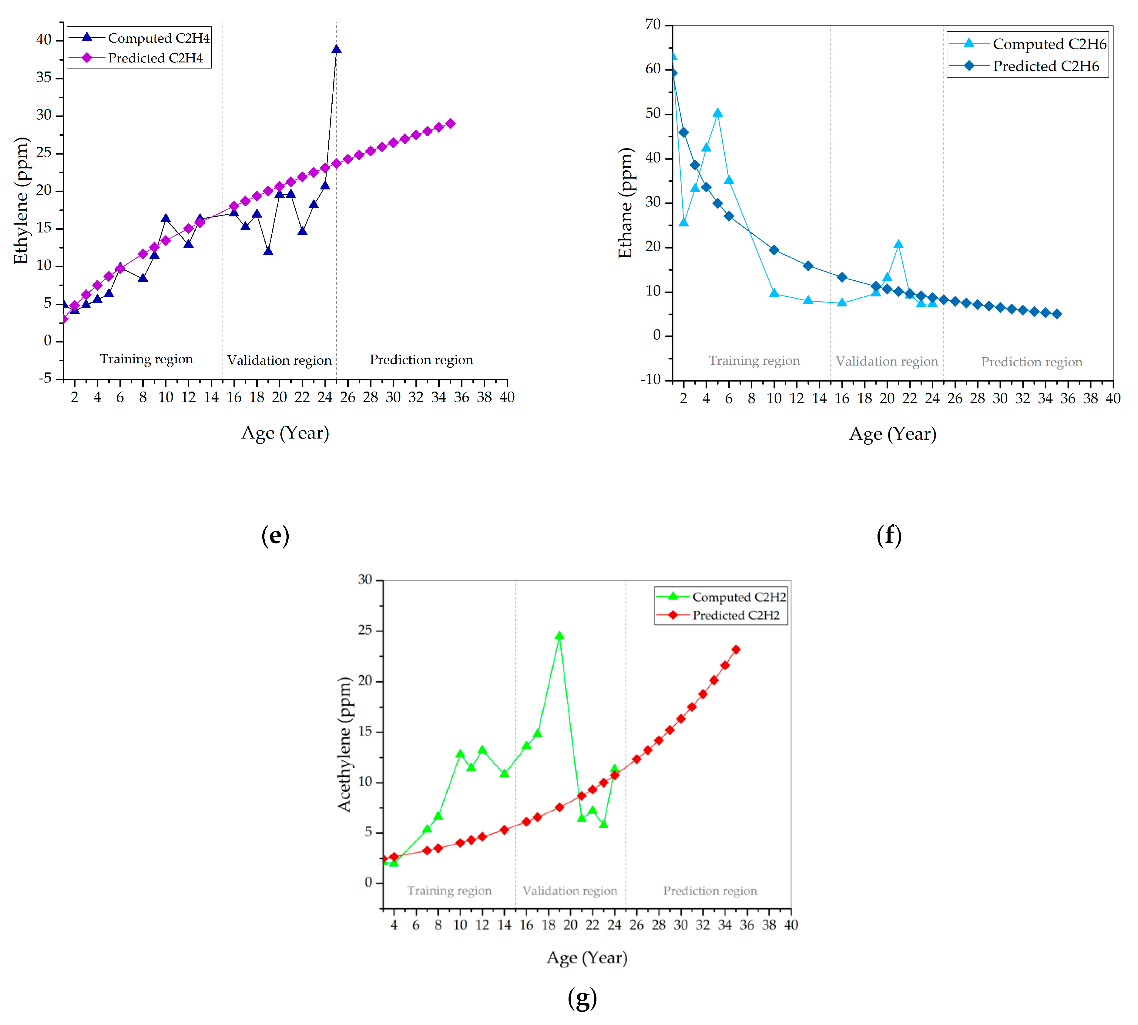
2.2. Condition Data Estimation

The condition parameters data represented by the Weibull and normal distributions were computed at the 50th percentile of sample data. Using the ICDF with the respective $\alpha$ and $\beta$, the data were evaluated at probability values, $p$. $p$, $\alpha$, and $\beta$ can be vectors, matrices, or multidimensional arrays with the same size [41]. A scalar input was expanded to a constant array of the same size as the other inputs. The ICDF of the Weibull distribution model at $p=0.5$ can be expressed in Equation (19) [42].

$$x=F^{-1}\left(\alpha ,\beta \right)=-\alpha {\left[ln\left(1-p\right)\right]}^{\frac{1}{\beta }}$$

(19)

Similarly, the condition parameters data that were represented by the normal distribution at $p=0.5$ from the data sample were computed using the ICDF, as shown in Equations (20) and (21).

$$x=F^{-1}\left(\mu ,\sigma \right)=\left\{x:F\left(\mu ,\sigma \right)=p\right\}$$

(20)

where

$$p=F\left(x|\mu ,\sigma \right)=\frac{1}{\sigma \sqrt{2\pi }}{{\displaystyle \int }}_{-\infty }^{x}ex{p}^{\frac{-{\left(t-\mu \right)}^2}{2{\pi }^2}}dt$$

(21)

2.3. Health Index Model Based on Scoring Algorithm

HI was computed based on a scoring algorithm. It is a conventional method that utilizes the weighting and ranking techniques to a list of condition parameters data, followed by conversion to scores from a predefined grade range. The scores were later aggregated into a single quantitative value. This method was employed due to its flexibility with the available data and it was the most commonly used by the utilities [1,2,3,4,5,6,43].

The condition parameters data were retrieved from the CBM database and the on-site physical conditions. The scoring and weighting algorithm is defined based on the technical guidelines, historical database, and fundamental theory. Expert decision and failure rate record are typically used to describe the appropriate weightages [1]. The procedures for determining the scores and weightage based on the different input parameters can be found in [1]. The final HI that was used in this study was computed according to Equation (23), which was adopted and modified from Equation (22) [1,43].

$$HI=60\%\times \frac{{{\displaystyle \sum }}_{j=1}^{21}{K}_{j}HI{F}_j}{{{\displaystyle \sum }}_{j=1}^{21}4K_j}+40\%\times \frac{{{\displaystyle \sum }}_{j=22}^{24}{K}_{j}HI{F}_j}{{{\displaystyle \sum }}_{j=22}^{24}4K_j}$$

(22)

The updated HI formula omitted the contribution factors from transformers (60%) and tap changer (40%) derived from CIGRÉ WG 12-05 [44]. Because this study only considered three parameters, namely dissolved gases, oil quality, and furfural condition parameters of transformers data.

$$HI=\frac{{{\displaystyle \sum }}_{j=1}^3{K}_{j}HI{F}_j}{{{\displaystyle \sum }}_{j=1}^{3}4K_j}=\frac{K_{DGA}HI{F}_{DGA}+K_{OQA}HI{F}_{OQA}+K_{FCA}HI{F}_{FCA}}{4K_{DGA}+4K_{OQA}+4K_{FCA}}$$

(23)

where $K$ is the coefficient that is assigned to the respective factor and HIF is the score of each factor. In this case, $K_{DGA}=10$, $K_{OQA}=$ 8, and $K_{FCA}=6$, respectively, and HIF is the rating (A, B, C, D, E) that is converted to a factor between 4 and 0 [1]. Finally, the HIs were categorized, as per Table 11 in [1], and grouped into discrete categories, from “very good” to “very poor”, which correspond to transformer condition and interpretations.

3. Case Study

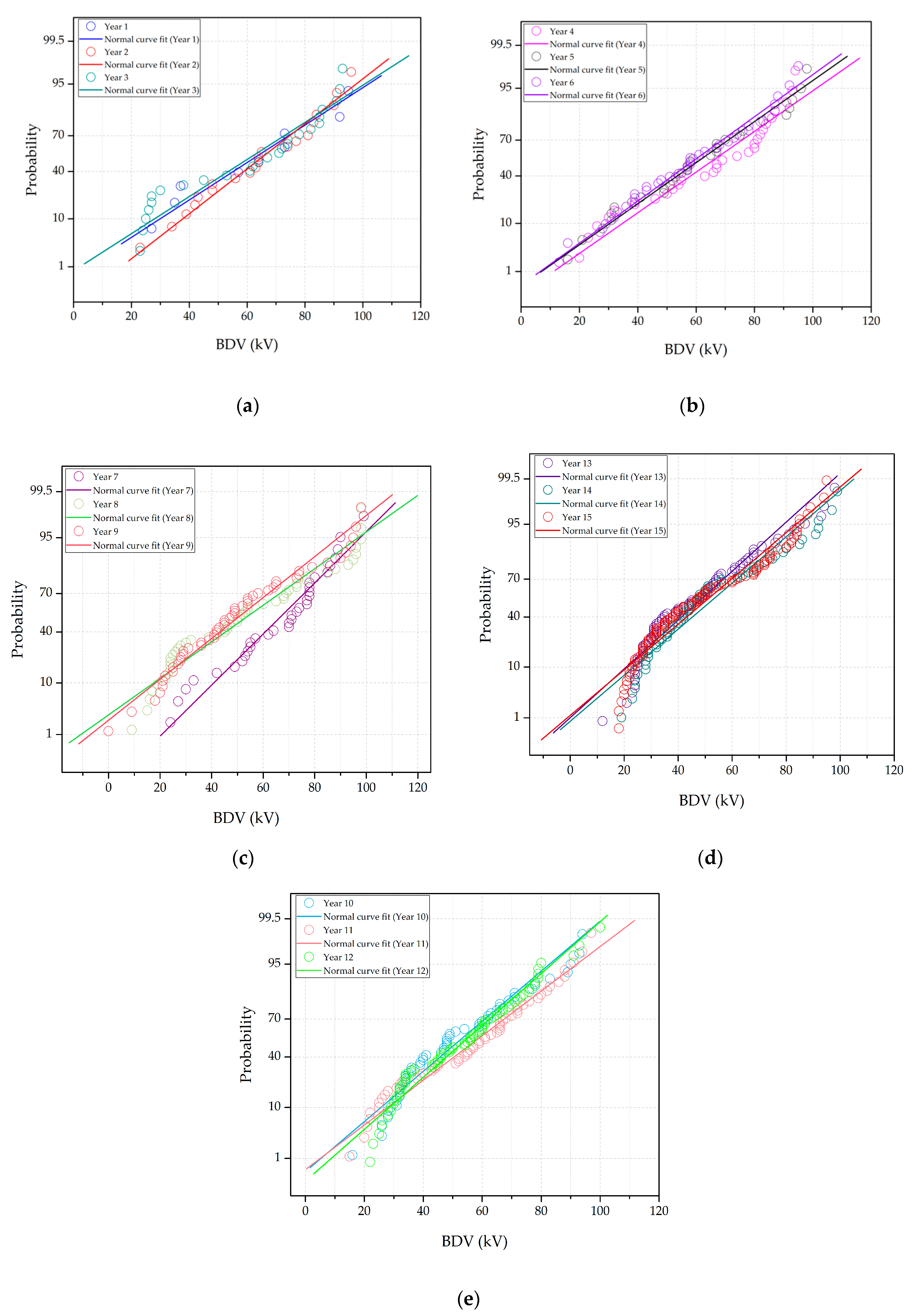
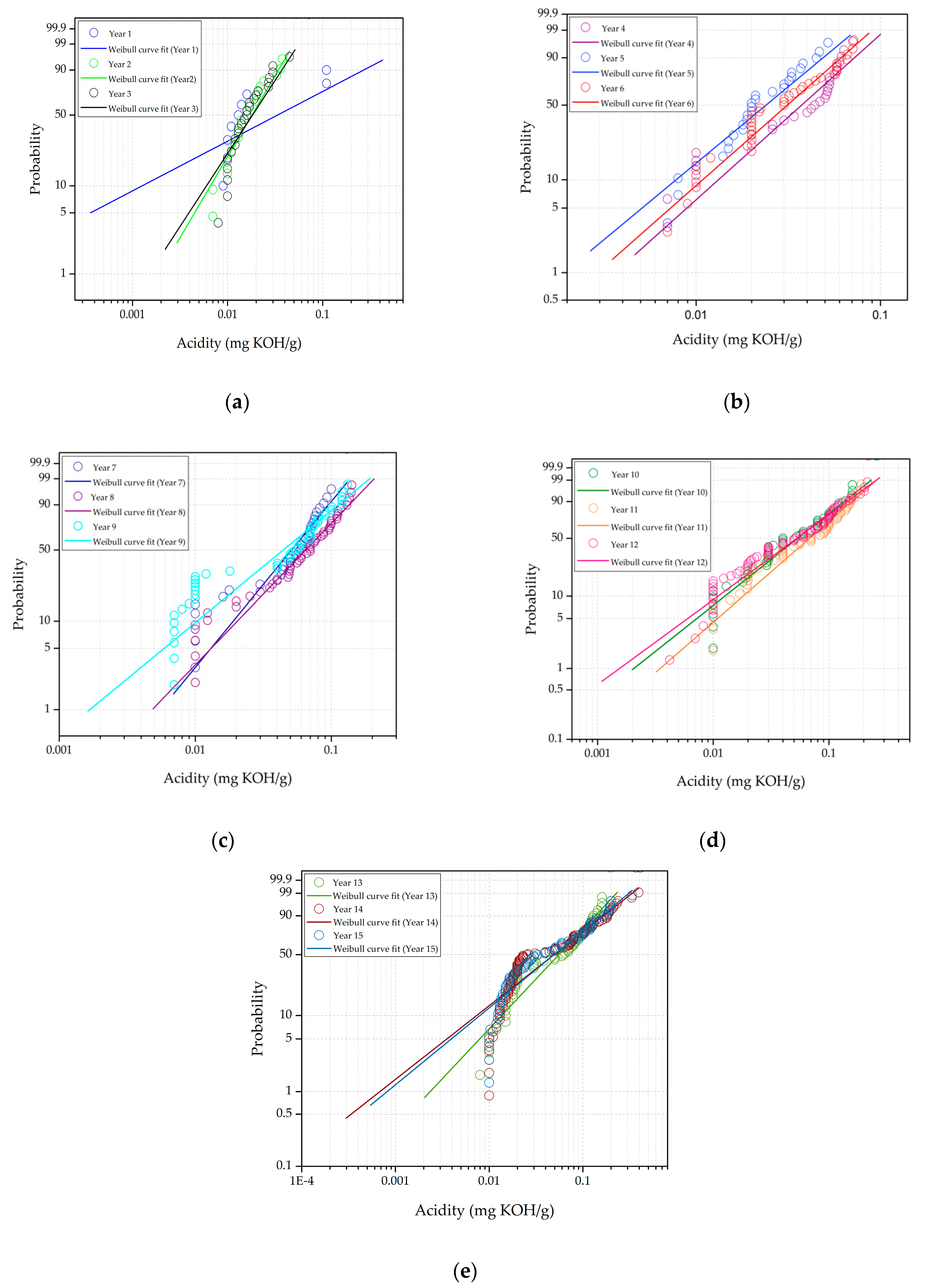
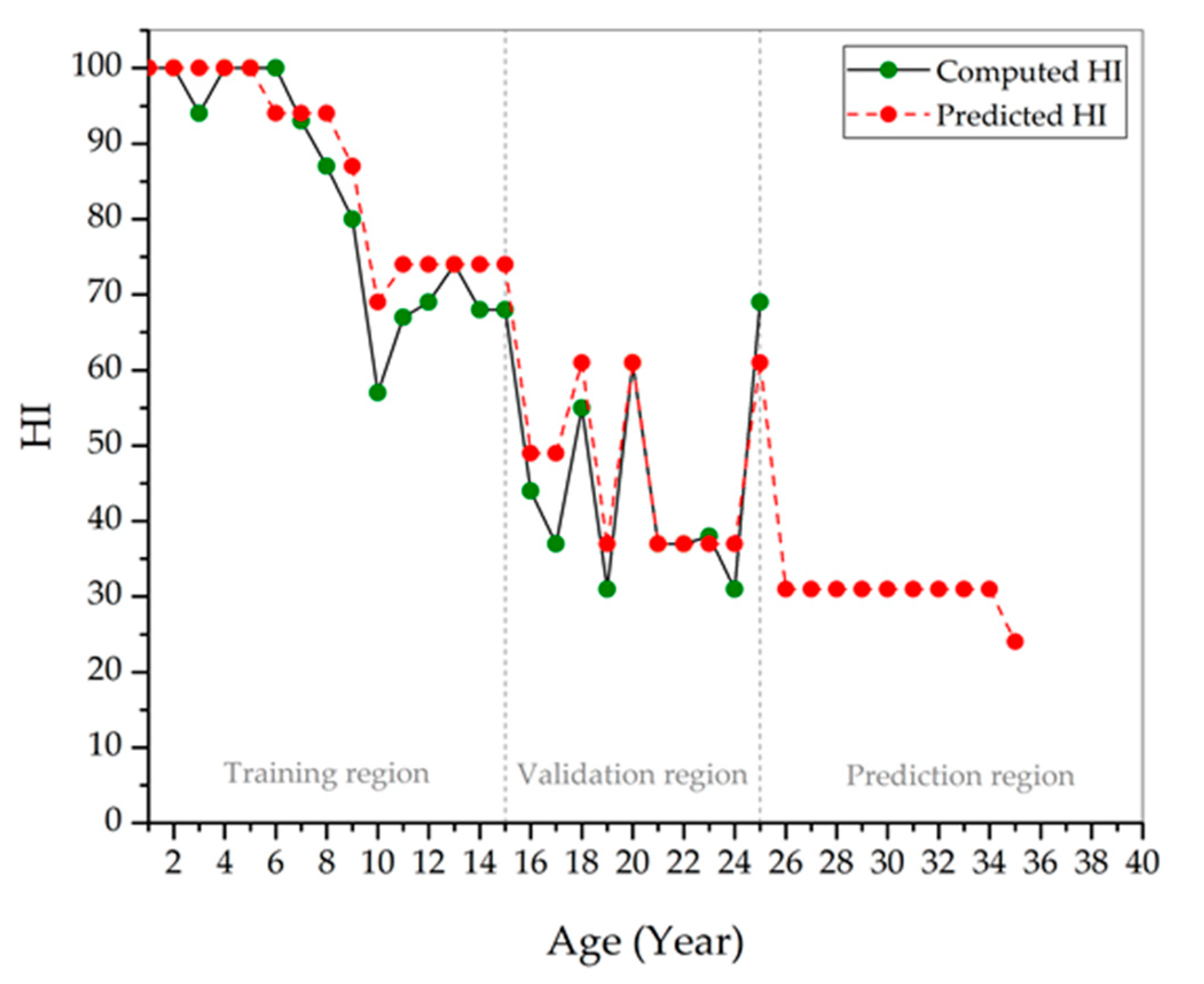
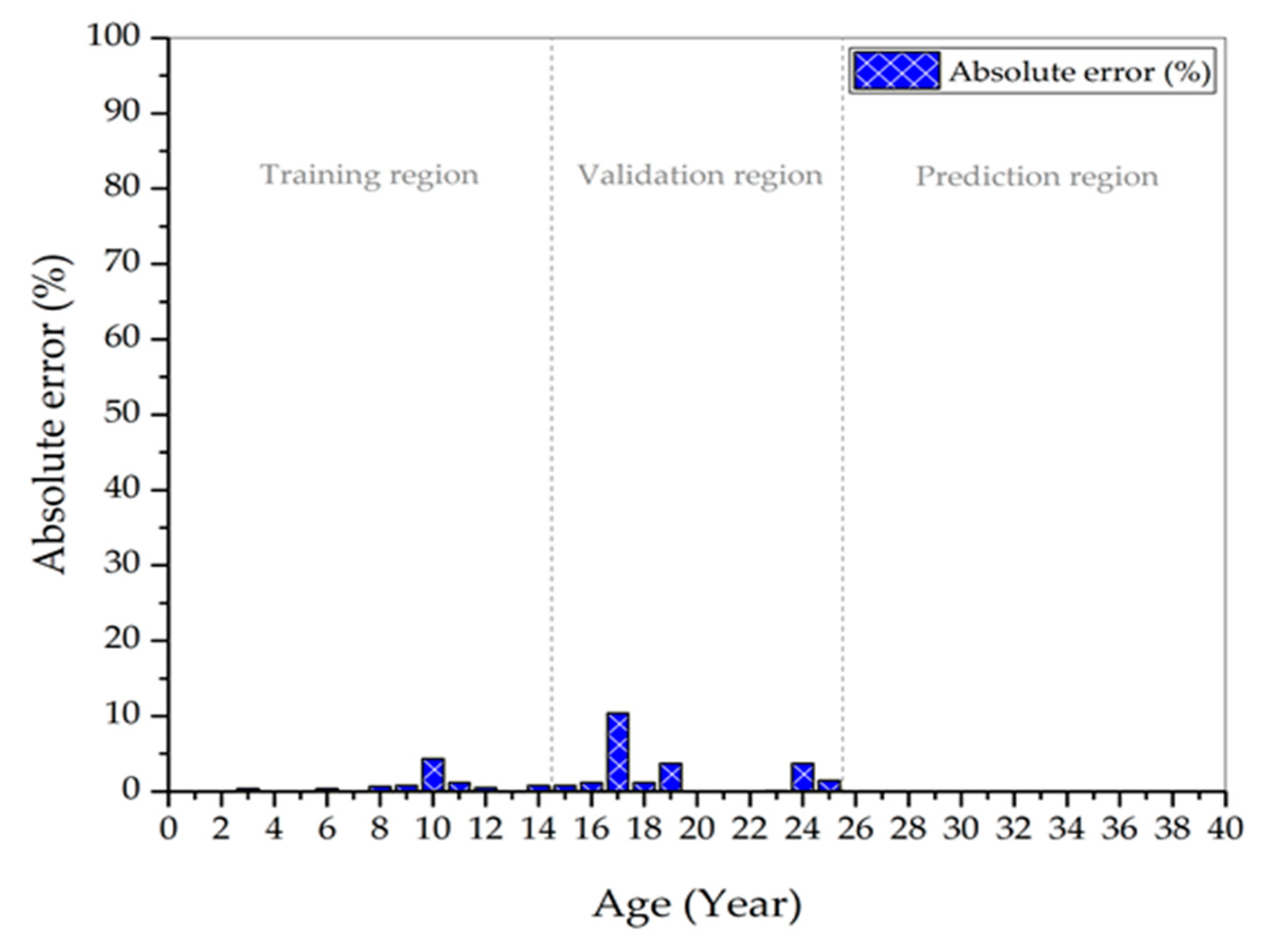
3.1. Implementation of Statistical Distribution Models to Transformer CBM Data

The condition parameters data that were used in the study were from 1322 oil samples (dataset) that contain 17,186 measurements data from 13 condition parameters data that were extracted from 373 distribution transformers. The data were divided into training (9425) and validation (7761) purposes. These transformers have voltage and power ratings of 33/11 kV (step-down) and 30 MVA, respectively. The age band of the data is from 1 to 25 years.

Table 1. Dataset distribution for each year.

Year	1	2	3	4	5	6	7	8	9	10	11	12	13	14
Dataset	9	22	26	30	32	37	33	49	52	52	56	77	76	61
Year	15	16	17	18	19	20	21	22	23	24	25	Total
Dataset	113	116	86	103	87	65	55	37	31	10	7	1322

tabulates the dataset distribution for each year.

Next, the condition parameters data were sorted, scaled logarithmically, and then plotted on the x-axis. The y-axis represents either Weibull or normal distribution quantiles, converted into probability values while using CDF Equations (2) and (4), respectively. Figure 2 and Figure 3 show the probability plots that were obtained for dielectric breakdown voltage and acidity from year 1 to 15, fitted by normal and Weibull distributions, respectively. Based on Figure 2a,b, the dielectric breakdown voltage data for year 1 to 2 and year 4 to 6 are close to the normal distribution fitting line. For year 3, the apparent deviation of the dielectric breakdown voltage data from the fitting line occurs at probabilities higher than 95% and between 10% and 40%. Significant deviations are also observed, particularly at probabilities less than 10% and above that 90%, as shown in Figure 2c–e for year 7 to 15.

Figure 3a–e plot the Weibull distribution fittings for acidity data. Apparent deviations can be observed at lower and upper tails of the Weibull distribution. The Weibull distribution could not represent the acidity data for year 1 quite well due to the large data variation within this period, as shown in Figure 3a. There are slight deviations of the acidity data from the Weibull distribution fitting at a probability less than 10% for year 2 to 3. The acidity data for year 4 to 6 could be represented quite well by the Weibull distribution, as shown in Figure 3b. The patterns of Weibull distribution fittings for year 7 to 9 and year 10 to 12 are quite similar, whereby apparent deviations of the acidity data occur at probabilities between 10% and 40%, as shown in Figure 3c,d. The acidity data for year 13 to 15 deviate from the Weibull distribution fittings at probability less than 40%. as shown in Figure 3e.

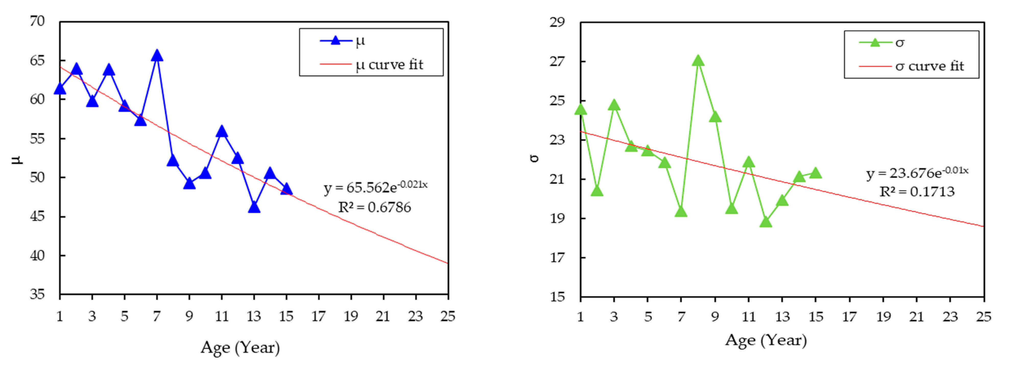
3.2. Distribution Parameters and Condition Data Estimations

Next, the distribution parameters for two-parametric Weibull and normal were computed based on (5)–(18).

Table 2. Computed distribution parameters for dielectric breakdown voltage and acidity.

Transformer Age	Dielectric Breakdown Voltage		Acidity
	$\mathit{\mu }$	$\mathit{\sigma }$	$\mathit{\alpha }$	$\mathit{\beta }$
1	61.444	24.587	0.0323	0.9318
2	64.000	20.459	0.0220	1.8741
3	59.808	24.832	0.0227	1.6902
4	63.862	22.696	0.0298	1.6803
5	59.250	22.489	0.0457	1.8153
6	57.460	21.898	0.0384	1.7849
7	65.727	19.391	0.0617	1.9102
8	52.265	27.099	0.0810	1.6304
9	49.308	24.218	0.0588	1.2918
10	50.654	19.531	0.0712	1.2977
11	56.000	21.916	0.0880	1.4233
12	52.605	18.849	0.0716	1.1990
13	46.324	19.959	0.0727	1.3391
14	50.656	21.168	0.0714	0.9885
15	48.566	21.355	0.0850	1.0715

tabulates an example of Weibull and normal distribution parameters fittings for dielectric breakdown voltage and acidity. For dielectric breakdown voltage data, the mean $\mu$ shows an apparent linear decrement trend as the transformer age increases. The standard deviation $\sigma$ only shows a slight decrement trend with the increment of transformer age. For the acidity data, the $\alpha$ initially fluctuates between 0.022 and 0.0323 for year 1–4. It starts to increase significantly as the transformer age increases from year 4 to year 10. After year 10, it stabilizes between 0.0712 and 0.085 after year 10. The $\beta$ for year 1 is relatively low as compared to other data and it is due to the poor fittings of Weibull distribution as shown in Figure 2a. Nonetheless, a decrement pattern is observed for the $\beta$ as the transformer age decreases.

Next, the distribution parameters from year 16 to 25 were fitted and extrapolated while using the curve fitting process based on the WLS method, as shown in Figure 4 and Figure 5. It is quite difficult to obtain high $R^2$ for all of the fittings due to the large variation of the distribution parameters. However, this limitation needs to be considered in this study in order to obtain the representative model for the transformer population. It is important to be noted, due to the nature of scoring and weighting HI technique used in this study, the variations of the individual condition parameters data will be less sensitive, since the calculation itself is based on aggregation method, whereby some of the values have a small effect on the overall model itself.

The exponential-based model was chosen for the curve fitting process, since it can provide the highest $R^2$ when compared to other models. For dielectric breakdown voltage data, the fittings of $\mu$ and $\sigma$ exponentially decrease as the transformer age is increased. Based on the extrapolation, the $\mu$ and $\sigma$ at year 25 are 35.005 and 18.434, respectively, as shown in

Table 3. Estimated distribution parameters for dielectric breakdown voltage and acidity.

Transformer Age	Dielectric Breakdown Voltage		Acidity
	$\mathit{\mu }$	$\mathit{\sigma }$	$\mathit{\alpha }$	$\mathit{\beta }$
16	43.877	20.170	0.0719	1.2458
17	42.790	19.970	0.0779	1.2175
18	41.729	19.771	0.0844	1.1898
19	40.695	19.574	0.0914	1.1627
20	39.686	19.379	0.0991	1.1363
21	38.702	19.187	0.1073	1.1105
22	37.743	18.996	0.1163	1.0852
23	36.807	18.807	0.1259	1.0605
24	35.895	18.619	0.1364	1.0364
25	35.005	18.434	0.1478	1.0129

. For the acidity data, the fitting of $\alpha$ increases exponentially as the transformer age increases. On the other hand, the fitting of the $\beta$ shows a slight decrement trend. Table 3 presents the estimated distribution parameters for dielectric breakdown voltage and acidity from year 16 to 25. Next, the individual condition parameters data for the next 10 years were computed while using the estimated distribution parameter through ICDF, as in Equations (19) and (20) for validation purpose.

Figure 6 presents the predicted and computed individual condition parameters data over the transformer age band. Based on Table 2 in [16], the predicted dielectric breakdown voltage is quite close to the computed dielectric breakdown voltage, whereby it stays in “very good” condition for 25 years, as shown in Figure 6a. Most of the predicted water content shows reasonable agreement with the computed water content throughout the transformer age period, as in Figure 6b. An apparent deviation is found between predicted and computed water content for year 8–10 and year 25. The predicted and computed water content remain in “very good” condition for 25 years. The predicted interfacial tension shows a clear deviation from the computed interfacial tension, as seen in Figure 6c. The predicted interfacial tension is in “very good” condition throughout the first seven years. From year 8 to 15, it is in “good” condition and ends up in “fair” condition after year 15. Meanwhile, the computed interfacial tension is in “very good” condition during the first four years. It fluctuates among “very good”, “good”, and “fair” conditions between year 5 and 9. It enters a “good” condition after year 9 and then transits to “fair” condition between year 17 and 21. After year 21, it fluctuates between the “very good” and “good” conditions. The predicted color is close to the computed color throughout the first 23 years, as shown in Figure 6d. It deviates from the computed color after 23 years. The predicted color is in “very good” condition throughout the first eight years and then transits to “good” condition from year 9 to 11. The predicted color enters a “fair” condition between year 12 and 15. After 15 years, it ends up in a “poor” condition. Meanwhile, the computed color is in “very good” condition during the seven years and it transits to “good” condition from year 8 to 10 and then enters “fair” conditions in year 11. Between year 12 and 13, the computed color reinstates to a “good” condition. It enters the “fair” condition between year 14 and 16, and later ends up in “poor” condition. There are deviations between predicted and computed acidities between year 7–12, 16–18, and 22–24, as shown in Figure 6e. The predicted acidity is in a “very good” condition during the first 15 years. It ends up in “good” condition after year 15. The computed acidity is in “very good” during the first six years. Between year 7 and 9, it fluctuates between “very good” and “good” conditions. After year 9, the computed acidity remains in “good” condition. The predicted 2-furfuraldehyde remains close to the computed 2-furfuraldehyde during the first 15 years, as shown in Figure 6f. Most of the predicted 2-FAL is lower than the computed 2-furfuraldehyde after year 10. The predicted and computed 2-FAL are in THE “very good” condition during the first five years. Between year 6 and 15, the predicted 2-FAL is in “good” condition. It ends up in “fair” condition after year 15. The computed 2-FAL is in “good” between year 8 and 13. After year 13, it enters “fair” conditions. It is in “poor” condition between year 18 and 19, and it reinstates to “good” condition between year 20 and 22. After 22 years, it remains in a “fair” condition.

Table 4. The representative distribution for oil quality and furfural analyses.

Parameter	Fitted Distribution	Master Curve Equation	${\mathit{R}}^2$
Dielectric breakdown voltage	Normal	y = exp(4.204 − 0.026x + 0.0001x2)	0.8379
Water content	Weibull	y = exp(2.181 + 0.423x − 0.0004x2)	0.6167
Interfacial tension	Weibull	y = exp(3.468 − 0.056x + 0.002x2)	0.3602
Color	Normal	y = 0.321(1 + x)0.727	0.9044
Acidity	Weibull	y = 0.015(1 + x)0.531	0.6224
2-FAL	Normal	y = 9.088x1.459	0.4674

summarizes the representative distribution models for each condition parameters data in oil quality and furanic compound analyses. The dielectric breakdown voltage, color, and 2-FAL can be represented by the normal distribution, whereas interfacial tension, acidity, and water content are suitable to be represented by Weibull distribution. Color has the highest $R^2$ with 0.9044, and interfacial tension has the lowest $R^2$ with 0.3602. The exponential-based model was chosen for the curve fitting process for dielectric breakdown, water content, and interfacial. Whereas, color, acidity, and 2-FAL could be curve fitted by the power-based model. These models are chosen, since the highest $R^2$ is obtained when compared to other models besides these curves depict the closest generic trends of oil quality and furanic compound analyses parameters data.

Most of the predicted dissolved gases show deviation with the computed dissolved gases, as shown in Figure 7. Based on Table 1 in [16], the predicted H₂ deviates from the computed H₂ during the first two years, between year 4–7 and 17–21, as shown in Figure 7a. Both of the predicted and computed H₂ maintain in “very good” condition for 25 years. The predicted CH₄ still follows the decrement trend of the computed CH₄, regardless of the deviation, as seen in Figure 7b. The predicted and computed CH₄ remains in “very good” condition for 25 years. A few of the predicted CO show reasonable agreement with the computed CO between year 4 and 23, as shown in Figure 7c. The deviation between the predicted and computed CO occurs between year 1–3 and year 24–25. The predicted CO maintains in “very good” condition during the first seven years and later transits to the “good” condition. The computed CO maintains in “very good” during the first six years. Between year 7 and 23, it is in “good” condition. The computed CO reinstates to the “very good” condition after 23 years. The majority of the predicted CO₂ deviates from the computed CO₂, as shown in Figure 7d. The predicted CO₂ is in “very good” condition during the first two years. It is in a “good” condition between year 3 and 7. After seven years, the predicted CO₂ remains in a “fair” condition. The computed CO₂ is in “very good” condition during the first three years. From year 4 to 6, the computed CO₂ is in “good” condition. It enters a “fair” condition after year 6. It reinstates to “good” condition between year 21 and 23, and later transits to “very good” condition. The predicted C₂H₄ is close to computed C₂H₄ during the first 24 years, as shown in Figure 7e. It deviates from computed C₂H₄ at year 25. Predicted and computed C₂H₄ both maintain in “very good” condition for 25 years. Apparent deviation between predicted and computed C₂H₆, as shown in Figure 7f. The predicted and computed C₂H₆ are in “very good” condition for 25 years. Similarly, the predicted C₂H₂ shows a clear deviation from the computed C₂H₂, as shown in Figure 7g. The predicted C₂H₂ is in “good” condition during the first 10 years. After year 8, the predicted C₂H₂ remains in “fair” conditions until 25 years. On the other hand, the computed C₂H₂ is in “good” condition during the first eight years. From year 10 to 19, the computed C₂H₂ is a “fair” condition. After year 19, it remains in “good” condition and later transits to “fair” condition after year 23.

Table 5. The representative distribution for dissolved gas parameters data.

Parameter	Fitted Distribution	Master Curve Equation	${\mathit{R}}^2$
H2	Weibull	y = exp(4.491 + 0.021x − 0.005x2)	0.5986
CH4	Weibull	y = exp(3.121 − 0.056 + 0.001x2)	0.4785
CO	Normal	y = −305.6exp0.017x	0.2375
CO2	Normal	y = 2000exp0.035x	0.5168
C2H4	Weibull	y = 2.183x0.732	0.6714
C2H6	Weibull	y = exp(4.090 − 0.135 + 0.002x2)	0.7155

summarizes the representative distributions for each of the dissolved gas parameters data. Based on the results, the majority of the dissolved gas parameters data fit Weibull distribution, except for C₂H₂, CO, and CO₂ fitting normal distribution. C₂H₆ has the highest $R^2$ with 0.7155 and CO₂ has the lowest $R^2$ with 0.2375. The exponential-based model was chosen for the curve fitting process for all dissolved gas parameters data, except for C₂H₄, which was curve fitted by the power-based model. The justification of the chosen distributions for dissolved gas parameters data is the same as the oil quality and furanic compound parameters data.

Figure 8 shows the predicted HI obtained by statistical model in Figure 6 and Figure 7 for a period of 25 years. It is observed that most of the predicted HI values are close to the computed HI. Based on Figure 9, there are considerably small deviations for the predicted HI at year 10, 19, and 24. The HI at year 17 recorded the highest deviation. Further hypothesis testing to measure the best-of-fit between the computed and predicted HI was performed while using the Chi-square statistic, as seen in Equation (24),

$$X^2={\displaystyle \sum }_{n=1}^{25}\frac{{\left(P_n-C_n\right)}^2}{C_n}$$

(24)

where $n$ is the total year of the transformer in term of age, $C_n$ is the computed HI at $n$ year, $P_n$ is the predicted HI at $n$ year, and $X^2$ is a Chi-square statistic coefficient with degree of freedom, $n-1$. The significance level $\alpha$ was set to 0.05, thus the rejection area fell after the critical value, which is 13.85. The $X^2$ of HI is 12.94, where, at $\alpha =0.05$, it falls outside the area of rejection.

The average percentage error between the predicted and computed HI was performed based on Equation (25).

$$Average percentage error (\%)= \frac{{{\displaystyle \sum }}_{n=1}^{25}\left(\frac{\left|C_n-P_n\right|}{\left|C_n\right|}\times 100\%\right)}{n}$$

(25)

where $C_n$ is the computed HI, $P_n$ is the predicted HI, and $n$ is the age of the transformer.

Figure 9 presents the absolute error percentages between the computed and predicted HIs that have been obtained based on SDM for 25 years. The overall average absolute error percentage in the training region is 0.65%, while, for the validation region, is 2.17%. The HI predicted using SDM for the transformers in validation region yields 97.83% accuracy. The application of SDM to predict HI of transformer population is a propitious approach for asset management in utilities. It is shown that, with limited historical condition parameters data, SDM is able to predict the transformers’ HI. These findings can be further validated if direct HI data from utilities can be acquired in the future. The application can be extended to another fleet or unit, regardless of ratings/sizes, because it is a data driven model. In addition, it is interesting to examine the HI model based on SDM to represent the condition of transformer due to oil change or regeneration that can be carried out as part of the future study.

4. Conclusions

In summary, it is found that the dielectric breakdown voltage, color, 2-FAL, CO, CO₂, and C₂H₂ under study could be represented by the normal distribution. The Weibull distribution is suitable for representing the IFT, acidity, water content, H₂, CH₄, C₂H₆, and C₂H₄. It is found that SDM can be utilized to estimate the HI of transformers while using individual condition parameters data. The predicted accuracy is subject to the obtainability of the data at various ages. Predominantly, the trends of the predicted HI are close to the computed HI. The hypothesis testing from the results using Chi-square shows that the $X^2$ value of HI data is 12.94, where it falls outside the rejection area at 0.05 significance level. The overall average percentages of absolute errors in training and validation regions are 0.65% and 2.17%, respectively. The predicted HI of transformers based on SDM yields accuracy of about 97.83%.

References

1. Jahromi, A.N.; Piercy, R.; Service, J.R.R.; Fan, W. An Approach to Power Transformer Asset Management Using Health Index. IEEE Electr. Insul. Mag. 2009, 25, 20–34. [Google Scholar] [CrossRef]
2. Scatiggio, F.; Pompili, M.; Calacara, L. Transformers Fleet Management Through the use of an Advanced Health Index. In Proceedings of the 2018 IEEE Electrical Insulation Conference (EIC), San Antonio, TX, USA, 17–20 June 2018; pp. 395–397. [Google Scholar] [CrossRef]
3. Haema, J.; Phadungthin, R. Condition Assessment of the Health Index for Power Transformer. In Proceedings of the 2012 Power Engineering and Automation Conference, Wuhan, China, 18–20 September 2012; pp. 1–4. [Google Scholar] [CrossRef]
4. Picher, P.; Boudreau, J.F.; Manga, A.; Rajotte, C.; Tardif, C.; Bizier, G.; Di Gaetano, N.; Garon, D.; Giard, B.; Hamel, J.F.; et al. Use of Health Index and Reliability Data for Transformer Condition Assessment and Fleet Ranking. In Proceedings of the Hydro-Québec, A2-101 CIGRE 2014, Paris, France, 24–29 August 2014. [Google Scholar]
5. Vermeer, M.; Wetzer, J.; van der Wielen, P.; de Haan, E.; de Meulemeester, E. Asset-Management Decision-Support Modeling, Using a Health and Risk Model. In Proceedings of the 2015 IEEE Eindhoven PowerTech, Eindhoven, The Netherlands, 29 June–2 July 2015; pp. 1–6. [Google Scholar]
6. Zaidey, Y.; Ghazali, Y.; Rosli, H.A. TNB Experience in Condition Assessment and Life Management. In Proceedings of the 20th International Conference and Exhibition on Electricity Distribution, Prague, Czech Republic, 8–11 June 2009; pp. 8–11. [Google Scholar]
7. Zec, F.; Kartalović, N.; Stojić, T. Prediction of High-Voltage Asynchronous Machines Stators Insulation Status Applying Law on Increasing Probability. Int. J. Electr. Power Energy Syst. 2019, 116, 105524. [Google Scholar] [CrossRef]
8. Feng, X.; Zhou, Y.; Hua, T.; Zou, Y.; Xiao, J. Contact Temperature Prediction of High Voltage Switchgear Based on Multiple Linear Regression Model. In Proceedings of the 2017 32nd Youth Academic Annual Conference of Chinese Association of Automation (YAC), Hefei, China, 19–21 May 2017; pp. 277–280. [Google Scholar] [CrossRef]
9. Manninen, H.; Kilter, J.; Landsberg, M. Health Index Prediction of Overhead Transmission Lines: A Machine Learning Approach. IEEE Trans. Power Deliv. 2021, 8977, 1–9. [Google Scholar] [CrossRef]
10. Li, G.; Wang, X.; Yang, A.; Rong, M.; Yang, K. Failure Prognosis of High Voltage Circuit Breakers with Temporal Latent Dirichlet Allocation. Energies 2017, 10, 1913. [Google Scholar] [CrossRef] [Green Version]
11. Shaban, K.B.; El-Hag, A.H.; Benhmed, K. Prediction of Transformer Furan Levels. IEEE Trans. Power Deliv. 2016, 31, 1778–1779. [Google Scholar] [CrossRef]
12. Jiang, J.; Chen, R.; Chen, M.; Wang, W.; Zhang, C. Dynamic Fault Prediction of Power Transformers Based on Hidden Markov Model of Dissolved Gases Analysis. IEEE Trans. Power Deliv. 2019, 34, 1393–1400. [Google Scholar] [CrossRef]
13. Qi, B.; Wang, Y.; Zhang, P.; Li, C.; Wang, H. A Novel Deep Recurrent Belief Network Model for Trend Prediction of Transformer DGA Data. IEEE Access 2019, 7, 80069–80078. [Google Scholar] [CrossRef]
14. El-Aal, R.A.A.; Helal, K.; Hassan, A.M.M.; Dessouky, S.S. Prediction of Transformers Conditions and Lifetime Using Furan Compounds Analysis. IEEE Access 2019, 7, 102264–102273. [Google Scholar] [CrossRef]
15. Yahaya, M.; Azis, N.; Mohd Selva, A.; Ab Kadir MZ, A.; Jasni, J.; Kadim, E.J.; Hairi, M.H.; Ghazali, Y.Z.Y. A Maintenance Cost Study of Transformers Based on Markov Model Utilizing Frequency of Transition Approach. Energies 2018, 11, 2006. [Google Scholar] [CrossRef] [Green Version]
16. Selva, A.M.; Azis, N.; Yahaya, M.S.; Ab Kadir MZ, A.; Jasni, J.; Yang Ghazali, Y.Z.; Talib, M.A. Application of Markov Model to Estimate Individual Condition Parameters for Transformers. Energies 2018, 11, 2114. [Google Scholar] [CrossRef] [Green Version]
17. Selva, A.M.; Yahaya, M.S.; Azis, N.; Kadir, M.Z.A.A.; Jasni, J.; Ghazali, Y.Z.Y. Estimation of Transformers Health Index Based on Condition Parameter Factor and Hidden Markov Model. In Proceedings of the 2018 IEEE 7th International Conference on Power and Energy (PECon), Kuala Lumpur, Malaysia, 3–4 December 2018; pp. 288–292. [Google Scholar] [CrossRef]
18. Ranga, C.; Chandel, A.K. Expert System for Health Index Assessment of Power Transformers. Int. J. Electr. Eng. Inform. 2017, 9, 850–865. [Google Scholar] [CrossRef]
19. Islam, M.M.; Lee, G.; Hettiwatte, S.N.; Williams, K. Calculating a Health Index for Power Transformers Using a Subsystem-Based GRNN Approach. IEEE Trans. Power Deliv. 2018, 33, 1903–1912. [Google Scholar] [CrossRef]
20. EKadim, J.; Azis, N.; Jasni, J.; Ahmad, S.A.; Talib, M.A. Transformers Health Index Assessment Based on Neural-Fuzzy Network. Energies 2018, 11, 710. [Google Scholar] [CrossRef] [Green Version]
21. Qureshi, M.S.; Swami, P.S.; Thosar, A.G. Prognostication of Health Index for Oil-Immersed Transformers Using Random Forest. Int. J. Sci. Technol. Res. 2019, 8, 1322–1329. [Google Scholar]
22. Ashkezari, A.D.; Ma, H.; Saha, T.K.; Ekanayake, C. Application of Fuzzy Support Vector Machine for Determining the Health Index of the Insulation System of In-service Power Transformers. IEEE Trans. Dielectr. Electr. Insul. 2013, 20, 965–973. [Google Scholar] [CrossRef] [Green Version]
23. Tee, S.; Liu, Q.; Wang, Z. Insulation Condition Ranking of Transformers through Principal Component Analysis and Analytic Hierarchy Process. IET Gener. Transm. Distrib. 2017, 11, 110–117. [Google Scholar] [CrossRef]
24. Elfarra, M.A.; Kaya, M. Comparison of Optimum Spline-Based Probability Density Functions to Parametric Distributions for the Wind Speed Data in terms of Annual Energy Production. Energies 2018, 11, 3190. [Google Scholar] [CrossRef] [Green Version]
25. Koizumi, D. On the Maximum Likelihood Estimation of Weibull Distribution with Lifetime Data of Hard Disk Drives. In Proceedings of the International Conference on Parallel and Distributed Processing Techniques and Applications (PDPTA’17); CSREA Press: Las Vegas, NV, USA, 2017; pp. 314–320. [Google Scholar]
26. Bala, R.J.; Govinda, R.M.; Murthy, C.S.N. Reliability Analysis and Failure Rate Evaluation of Load Haul Dump Machines Using Weibull Distribution Analysis. Math. Model. Eng. Probl. 2018, 5, 116–122. [Google Scholar] [CrossRef]
27. Verma, A.; Narula, A.; Katyal, A.; Yadav, S.K.; Anand, P.; Jahan, A.; Pruthi, S.K.; Sarin, N.; Gupta, R.; Singh, S. Failure Rate Prediction of Equipment: Can Weibull Distribution Be Applied to Automated Hematology Analyzers? Clin. Chem. Lab. Med. 2018, 56, 2067–2071. [Google Scholar] [CrossRef]
28. Xia, X.; Chang, Z.; Zhang, L.; Yang, X. Estimation on Reliability Models of Bearing Failure Data. Math. Probl. Eng. 2018, 2018, 6189527. [Google Scholar] [CrossRef] [Green Version]
29. Badune, J.; Vitolina, S.; Maskalonok, V. Methods for Predicting Remaining Service Life of Power Transformers and Their Components. Power Electr. Eng. 2013, 31, 123–126. [Google Scholar]
30. Zhou, D. Transformer Lifetime Modelling Based on Condition Monitoring Data. Int. J. Adv. Eng. Technol. 2013, 6, 613–619. [Google Scholar]
31. Barabadi, A.; Ghodrati, B.; Barabady, J.; Markeset, T. Reliability and Spare Parts Estimation Taking into Consideration The Operational Environment—A Case Study. In Proceedings of the 2012 IEEE International Conference on Industrial Engineering and Engineering Management, Hong Kong, China, 10–13 December 2012; pp. 1924–1929. [Google Scholar] [CrossRef]
32. Kontrec, N.; Panić, S. Spare Parts Forecasting Based on Reliability. Syst. Reliab. 2017. [Google Scholar] [CrossRef] [Green Version]
33. Bhattacharya, P.; Bhattacharjee, R. A Study on Weibull Distribution for Estimating the Parameters. Wind Eng. 2009, 33, 469–476. [Google Scholar] [CrossRef]
34. Zhou, D. Comparison of Two Popular Methods for Transformer Weibull Lifetime Modelling. Int. J. Adv. Res. Electr. Electron. Instrum. Eng. 2013, 2, 1170–1177. [Google Scholar]
35. Bowling, S.R.; Khasawneh, M.T.; Kaewkuekool, S.; Cho, B.R. A Logistic Approximation to the Cumulative Normal Distribution. J. Indutrial Eng. Manag. 2013, 2, 114–127. [Google Scholar] [CrossRef] [Green Version]
36. Yerukala, R.; Boiroju, N.K. Approximations to Standard Normal Distribution Function. Int. J. Sci. Eng. Res. 2015, 6, 2015. [Google Scholar]
37. Pobočíková, I.; Sedliačková, Z. Comparison of Four Methods for Estimating the Weibull Distribution Parameters. Appl. Math. Sci. 2014, 8, 4137–4149. [Google Scholar] [CrossRef]
38. Van Gelder, P.H.A.J.M. Statistical Methods for the Risk-Based Design of Civil Structures; Technische Universiteit Delft: Delft, The Netherlands, 2000; Volume 100. [Google Scholar]
39. Ruhi, S.; Sarker, S.; Karim, M.R. Mixture Models for Analyzing Product Reliability Data: A Case Study. Springerplus 2015, 4, 1–14. [Google Scholar] [CrossRef] [PubMed] [Green Version]
40. Chu, Y.K.; Ke, J.C. Computation Approaches for Parameter Estimation of Weibull Distribution. Math. Comput. Appl. 2011, 16, 702–711. [Google Scholar] [CrossRef] [Green Version]
41. Pishro-Nik, H. Introduction to Probability, Statistics, and Random Processes; Kappa Research, LLC: Blue Bell, PA, USA, 2014. [Google Scholar]
42. Yang, P.; Pan, S.; Jiang, J.; Rao, W.; Qiao, J. DGA and Weibull Distribution Model-based Transformer Fault Early Warning. IOP Conf. Ser. Mater. Sci. Eng. 2019, 569, 032072. [Google Scholar] [CrossRef]
43. Yahaya, M.S.; Azis, N.; Kadir, M.Z.A.A.; Jasni, J.; Hairi, M.H.; Talib, M.A. Estimation of Transformers Health Index Based on the Markov Chain. Energies 2017, 10, 1824. [Google Scholar] [CrossRef] [Green Version]
44. CIGRE-WG 12-05: An International Survey on Failures in Large power Transformers in Service. Electra 1983, 88, 21–48.
Figure 1. Modelling framework for future health index of the transformer population.
Applsci 11 02728 g001
Figure 2. Normal distribution probability plot for dielectric breakdown voltage from year (a) 1 to 3; (b) 4 to 6; (c) 7 to 9; (d) 10 to 12; and, (e) 13 to 15.
Applsci 11 02728 g002
Figure 3. Weibull distribution probability plot for acidity from year (a) 1 to 3; (b) 4 to 6; (c) 7 to 9; (d) 10 to 12; and, (e) 13 to 15.
Applsci 11 02728 g003
Figure 4. Parameters estimation for dielectric breakdown voltage based on the normal distribution model.
Applsci 11 02728 g004
Figure 5. Parameters estimation for acidity based on Weibull distribution model.
Applsci 11 02728 g005
Figure 6. Comparison between computed and predicted (a) dielectric breakdown voltage; (b) water content; (c) interfacial tension; (d) color; (e) acidity; and, (f) 2-furfuraldehyde.
Applsci 11 02728 g006
Figure 7. Comparison between computed and predicted (a) hydrogen; (b) methane; (c) carbon monoxide; (d) carbon dioxide; (e) ethylene; (f) ethane; and, (g) acetylene.
Applsci 11 02728 g007aApplsci 11 02728 g007b
Figure 8. Comparison between computed and predicted health index.
Applsci 11 02728 g008
Figure 9. The absolute error percentage between the computed and predicted health index.
Applsci 11 02728 g009