Abstract
Software is playing the most important role in recent vehicle innovations, and consequently the amount of software has rapidly grown in recent decades. The safety-critical nature of ships, one sort of vehicle, makes software quality assurance (SQA) a fundamental prerequisite. Just-in-time software defect prediction (JIT-SDP) aims to conduct software defect prediction (SDP) on commit-level code changes to achieve effective SQA resource allocation. The first case study of SDP in the maritime domain reported feasible prediction performance. However, we still consider that the prediction model has room for improvement since the parameters of the model are not optimized yet. Harmony search (HS) is a widely used music-inspired meta-heuristic optimization algorithm. In this article, we demonstrated that JIT-SDP can produce better performance of prediction by applying HS-based parameter optimization with balanced fitness value. Using two real-world datasets from the maritime software project, we obtained an optimized model that meets the performance criterion beyond the baseline of a previous case study throughout various defect to non-defect class imbalance ratio of datasets. Experiments with open source software also showed better recall for all datasets despite the fact that we considered balance as a performance index. HS-based parameter optimized JIT-SDP can be applied to the maritime domain software with a high class imbalance ratio. Finally, we expect that our research can be extended to improve the performance of JIT-SDP not only in maritime domain software but also in open source software.
1. Introduction
Nowadays software in various industries is an important and dominant driver of innovation. The amount of software continues to grow to deal with demands and challenges such as electrification, connectivity, and autonomous operations in vehicle industries [1]. The maritime domain is also confronting similar engineering challenges [2,3,4].
Software quality is the foremost concern in both software engineering and vehicle industries. Software quality assurance (SQA) is one of the prerequisites for maintaining such software quality owing to the safety-critical nature of vehicles. In particular, due to pressure and competition in these industries (i.e., tradeoff relationship among time, cost, and quality), effectual allocation of quality assurance (QA) resources to detect defects as quickly as possible in the early stages of the software lifecycle has become critical to reduce quality costs [5,6].
Just-in-time software defect prediction (JIT-SDP) aims to conduct software defect prediction (SDP) on commit-level code changes to achieve effective SQA resource allocation [7]. By pointing out potentially defect-prone modules in advance, SQA team allocates more efforts (e.g., spending more time on designing test cases or concentrating on more code inspection) on these identified modules [8]. SDP techniques are actively studied and developed to minimize time and cost in maintenance and testing phases in the software lifecycle. Machine learning and deep learning are widely used to predict defects in newly developed modules using models that are learned from past software defects and update details (e.g., commit id, committer, size, data and time, etc.) [9,10,11,12,13].
A previous case study [14] in the maritime domain discussed the fact that, as ships are typically ordered and constructed in series with protoless development, defects are prone to be copied on all ships in series once they occur. In comparison, the cost of removing defects is very high due to the global mobility of ships and restricted accessibility for defect removal. Due to these characteristics of the domain, the residual software defects should be minimized in order to avoid high post-release quality cost. The results of the case study showed that SDP can be applied effectively to allocate QA resources with feasible prediction performance with an average accuracy of 0.947 and f-measure of 0.947 yielding post-release quality cost reduction of 37.3%. The case study of SDP in the maritime domain showed feasible prediction performance and the best model was constructed using a random forest classifier. However, we still believe that the prediction model has room for improvement since the parameters’ optimization in the model have not been considered so far. For this problem, we mainly consider parameter optimization for bagging of decision trees as a base classifier with balanced fitness value which consider class imbalance distribution.
In this article, we demonstrated that performance of JIT-SDP can be improved by applying harmony search-based parameter optimization in an industrial context. Harmony search (HS) is a population-based meta-heuristic optimization algorithm, proposed by Geem et al. [15]. The algorithm imitates the design of a unique harmony in music to solve optimization problems. Its applications across an enormous range of engineering problems, such as power systems, job shop scheduling, congestion management, university timetables, clustering, structural design, neural networks, water distribution, renewable energy, data mining, and software have provided excellent results [16,17,18,19,20,21,22,23,24].
This article investigates the following research questions:
- RQ1: How much can HS-based parameter optimization improve SDP performance in maritime domain software?
- RQ2: By how much can HS-based parameter optimization method reduce cost?
- RQ3: Which parameters are important for improving SDP performance?
- RQ4: How does the proposed technique perform in open source software (OSS)?
The main contributions of this article are summarized as follows:
- To the best of our knowledge, we first apply HS-based parameter optimization to JIT-SDP and the maritime domain.
- We first apply HS-based parameter optimization with search space of the decision tree and bagging classifier together with balanced fitness function in JIT-SDP.
The remainder of this article is organized as follows. Section 2 explains the context of the maritime domain application and the HS algorithm. Section 3 describes the application of the JIT-SDP tailored parameter based on HS in the maritime domain. Section 4 discusses the experimental setup and research questions. The experimental results are analyzed in Section 5. Section 6 and Section 7 deal with the discussion and threats to validity, respectively. Section 8 explains the related work of this study. Finally, Section 9 concludes this article and points out some future work.
2. Background
This section describes the background in two main areas: (1) software practices and unique characteristics in the maritime domain, and (2) HS, which is used for parameter optimization.
2.1. Software Practices and Unique Characteristics in the Maritime Domain
The maritime and ocean transport industry is essential as it is responsible for the carriage of almost 90% of international trade. In large ships (i.e., typical type of maritime transportation), various equipment is installed to ensure flotation, mobility, independent survival, safety, and performance suitable for their intended use. Large ships also have cargo loading space, crew’s living space, an engine room for mobility, as well as more than three control rooms for operators to control the ship’s navigation, machinery, and cargo. Each control room has integrated systems, including workstations, controllers, displays, networks, and base/application software. These are networked systems with many types of sensor, actuator, and other interface systems, in accordance with their assigned missions. Each system or remote controllers can be acquired from various venders, and are integrated, installed and tested by an integrator. Only after an independent verifier audit-required tests can the ship be delivered to the customer.
Software plays significant roles in handling human inputs and interactions while coordinating essential control logic and/or tasks dependent on external input and output. With the emerging innovative future ships, the value of software continues to rise. Future maritime applications, for instance, can enable connectivity and autonomous operation including identification of obstacles in the environment [3,4]. The software-intensive systems installed on large ships include an integrated navigation system, engineering automation system, power generation or propulsion engine control system and cargo control system, each of which contains tens to hundreds of thousands of lines of source code. All systems installed to vehicles including ships need to be certified by a relevant certification authority when they are first developed, upgraded, or actually installed. The process of obtaining approval of a sample of the developed system from the authorized agency is referred to as type approval. Provided that the defined design or operating environment is identical, the same copy or product of a sample which was previously authorized can be approved as well [14].
Software development practices in the maritime and ocean transportation industry have not received much attention despite differences from other domains. Not only are they completely different from the IT development environment, but they are also very different from other vehicle industries; they constantly move around the world.
In short, there are three main characteristics [14].
- In general, ships are made to order and built in series with protoless development.
- Ships move around the world and have low accessibility for defect removal activities.
Figure 1 illustrates an example of how to induce a bug and duplicate it to multiple ships and removals during the manufacturing and operation of ships in series. The maritime and ocean industry is a conventional made-to-order industry that builds and delivers ships and offshore infrastructure that customers want. The fact that ships are mainly planned and constructed in sequence indicates that those same sister ships are virtually identical. Although ships do not have a prototype, the system, including the software, is tested during production to ensure that the predefined functions are working correctly [14]. As a result, various software installed onboard the ships shall be able to adapt or update functions promptly in advance or upon urgent adjustment requirements. Although most of the defects are avoided and prevented during testing, the characteristics of the maritime domain make it possible that defects will be induced into a whole series of ships until the bug is revealed and fixed if they are not found during testing. While defects detection is aimed in the test process to improve software quality and reduce cost, some defects are exploited in the operating phase. It can be very costly to patch such late-detected defects.
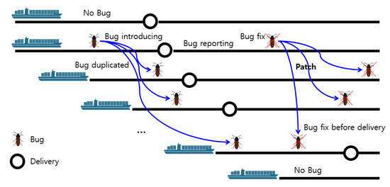
Figure 1.
Case of bug inducing and removing during the development and service of ships in series.
Once a ship is constructed and delivered to the ship owner, the ship will carry passengers and/or cargo while navigating designated or irregular routes. Ships travel around the world according to the route they operate. In the general IT environment, distribution or update of software through the internet or an automated distribution system are very common activities during deployment. However, in the maritime domain, an engineer would get to work on a ship at least once. If defects occur, the activity and visit of the engineer to the ship increases accordingly, raising the costs of installation and maintenance. The complexity of the service engineer’s job encompasses not just the time spent working on software, but also the time spent entering and leaving the shipyard and getting on the ship, and the unavoidable time spent. In addition, in order for a service engineer to visit the ship after the delivery, he/she must monitor the arrival and departure schedule of the ship, while taking into account the cost of overseas travel, ways to access to the port and to get on a ship, and unexpected changes of the schedule of the ship; it is common to wait one or two days or go to another port to get on a ship due to the delay in the schedule as depicted in Figure 2.
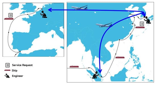
Figure 2.
Ship’s mobility around the world.
2.2. Harmony Search
The harmony search algorithm (HSA) is a population-based meta-heuristic optimization algorithm that imitates the music improvisation process where instrument players search the best harmony with repeated trails considering their experience [15]. Table 1 shows the parameters on which the HSA works. Harmony is a set of notes that each instrument player has decided. The harmony is stored in the harmony memory (HM) as an experience where each instrument player can refer to. A harmony memory size (HMS) indicates the maximum number of harmonies that instrument players can refer to. Whenever a new harmony is generated, each instrument player decides their own note considering a harmony memory considering rate (HMCR), a pitch adjusting rate (PAR), and a fret width (FW). HMCR is the probability that each player refers to a randomly selected harmony in the HM. PAR is the probability of adjusting a harmony that was picked from HM. FW is the bandwidth of the pitch adjustment. [25,26] The overall HS process iterates the maximum improvisation (MI) number of consecutive trails.

Table 1.
Parameters of harmony search.
Figure 3 describes overall process of the HSA. We supposed each harmony consists of N instrument player, and HMS consists of M harmony.
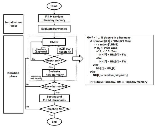
Figure 3.
Overall process of harmony search.
- (1)
- Initialization phase: The HS process starts from generating HMS number of randomly generated harmonies, and evaluate performance of the generated harmonies.
- (2)
- Iteration phase:
- The iteration phase starts from improvising a new harmony. Each instrument player decides their notes considering HMCR, PAR, and FW. The pseudocode for these functions is described in the right side of the Figure 3. Finally, this phase evaluates the newly improvising harmony.
- HSA generates M new harmonies, and updates the harmony memory with the new solution which is superior to the worst solution within the HM.
- The A and B processes iterate until the iteration is reached to the MI.
The main advantages of the HSA are clarity of execution, record of success, and ability to tackle several complex problems (e.g., power systems, job scheduling, congestion management) [16,17,18]. Another reason for its success and reputation is that the HSA can make trade-offs between convergent and divergent regions. In the HSA rule, exploitation is primarily adjusted by PAR and FW, and exploration is adjusted by the HMCR [19].
3. Harmony Search-Based Parameter Optimization (HASPO) Approach
Figure 4 shows the conceptual context of applying JIT-SDP in the maritime industry.
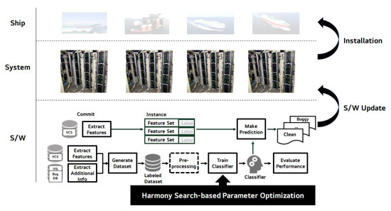
Figure 4.
Application of harmony search-based parameter optimized just-in-time software defect prediction (JIT-SDP).
The overall context of HS-based parameter optimized JIT-SDP in the maritime domain is as follows [14]:
- Data source preparation: sources of datasets such as version control systems (VCSs), issue tracking systems (ITSs), and bug databases are managed and maintained by software archive tools. The tools automate and facilitate the next feature extraction and a whole SDP process.
- Feature extraction: this step extracts instances that contain set of features and class labels, i.e., buggy or clean, from the VCSs. The feature set, so-called prediction metrics, play a dominant role in the construction of prediction models. In this article, we picked 14 change-level metrics [7] as a feature set and the class label as either buggy or clean in the binary classification. The reason we used the process metrics is the quick automation of the features and labels and the opportunity to make a prediction early in the project.
- Dataset generation: dataset with instances which were extracted in the previous step can be generated. For each change commit, an instance can be created. In this stage, practitioners relied on a SZZ tool [27] to extract datasets with 14 change-level metrics from the VCS. The detailed explanation can be referred to the original article [14].
- Preprocessing: preprocessing is a step in-between data extraction and model training. Each preprocessing technique (e.g., standardization, selection of features, elimination of outliers and collinearity, transformation and sampling) may be implemented independently and selectively [28]. Representatively, the over-sampling methods of the minority class [29] or under-sampling from the majority class can be used to work with the class imbalance dataset (i.e., the class distribution is uneven).
- Model training with HS-based parameter optimization and performance evaluation: this step is the main contribution of our article. Normally, classifiers can be trained based on the dataset collected previously. The existing ML techniques have been facilitated many SDP approaches [30,31,32,33]. The classifier with the highest performance index is selected by evaluating the performance in terms of balance which reflects class imbalance. A previous case study [14] in the maritime domain showed the best model was constructed using a random forest classifier. Optimizing the parameters of the predictive model was expected to improve the performance of the existing technique. For this problem, we mainly consider HS-based parameter optimization for bagging of decision trees as a base classifier. The detailed explanations of our approach, search space and fitness function are described in Section 3.1 and Section 3.2.
- Prediction: the proposed approach successfully builds a prediction model to determine whether or not a software modification is defective. Once the developer has made a new commit, the results of the prediction have been labeled as either buggy or clean.
3.1. Optimization Problem Formulation
In this section, we formulate our parameter optimization problem in JIT-SDP.
JIT prediction models can be constructed by a variety of machine learning classifiers (e.g., decision tree and bagging in this paper). Each machine learning classifier has a given list of parameters with a default value. For example, a random forest classifier has the number of decision trees with default 100 [34]. The result of prediction Y can be represented as function F of new commits Xi and a list of parameters P. i.e., Y = F (Xi, P)
Objective function. The performance of prediction result Y can be evaluated as mean of balances defined as: B = , where PD is Probability of Detection and PF is Probability of False Alarm, described in Section 4.3.
Parameter. Parameters P selected for optimization are listed in Table 2. The whole candidate parameters and their description are listed in Table A1 and Table A2 in Appendix A and Appendix B. Among the parameters in Table A1 and Table A2, we selected parameters for optimization by excluding the following parameters, respectively:
Table 2.
Search space, range, and interval of harmony search.
- (1)
- random_state in both classifiers is not selected because we already separated training and test dataset randomly before training.
- (2)
- min_impurity_split for a decision tree is not selected because it has been deprecated.
- (3)
- warm_start, n_jobs, verbose for bagging are not selected because they are not related to prediction performance.
The constraints for each parameter are listed in “range” column in Table 2. In the “interval” column of the table, “By HSA” means the interval is adjusted using FW by the HSA.
Our problem is computationally intensive. i.e., over 67,200,000 discrete candidates × 10 stratified × (2 × 5 + 6) cases. Thus, it is necessary to find optimal performance in a limited time and computation power through a heuristic approach [35].
3.2. Harmony Search-Based Parameter Optimization of JIT-SDP
Figure 5 is the overall process of the proposed HS-based parameter optimization for JIT-SDP. The process consists of two parts: updating harmony memory and getting fitness values.
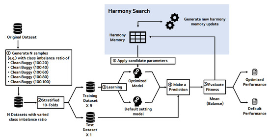
Figure 5.
Detailed process of harmony search-based parameter optimization.
The detailed process of HS-based parameter optimization is as follows:
- In step 1, N datasets (e.g., five datasets in this article), which have different class imbalance ratio, are generated. The reason for changing the class imbalance ratio between defects and non-defects in N steps is to show that this approach can be applied in various data distributions.
- In step 2, N datasets are divided into 9 training datasets and a test dataset for a stratified 10-fold cross-validation. The stratified method divides a dataset, maintaining the class distribution of the dataset so that each fold has the same class distribution as the original dataset [36].
- Step 3 makes a prediction model with a training set on a set of parameters, i.e., the harmony, in a harmony memory. We have 10 training and test sets, and thus can make nine more prediction models with the same set of parameters.
- Each 10 generated models predict the outcome of each test dataset matched to the model and extracts the confusion matrix to calculate each model’s balance performance in step 4.
- Step 5 calculates the mean of 10 balance values and store it in the harmony memory as a harmony’s fitness value.
- Finally, it updates harmony memory and applies the harmony to the prediction model, and iterates as many times as MI.
Harmony memory is a crucial factor of HSA. The harmony memory is where the top HMS harmonies of all generated harmony are stored, and newly generated harmonies are referred to the harmony memory for selecting search direction globally and locally. Figure 6 is a brief summary of the harmony memory of the proposed method.
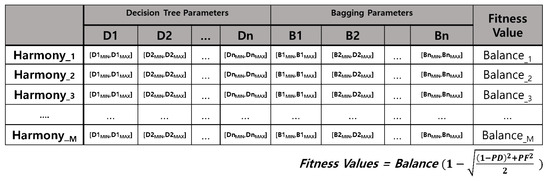
Figure 6.
Brief summary of harmony memory applying parameters.
Harmony memory is composed of the number of harmonies (i.e., HMS), which is M in the Figure 6. Each harmony consists of the parameter values of variables and a fitness value presenting the harmony’s goodness. A harmony has 17 variables; 11 decision tree parameters and 6 bagging parameters, and each variable is between minimum and maximum, which each parameter can have. Each harmony’s fitness value is the balance of the prediction model, which is generated using the harmony.
4. Experimental Setup
This section explains the experimental setup to address our research questions.
4.1. Research Questions
- RQ1: How much can HS-based parameter optimization improve SDP performance in maritime domain software?
- RQ2: By how much can HS-based parameter optimization method reduce cost?
- RQ3: Which parameters are important for improving SDP performance?
- RQ4: How does the proposed technique perform in Open Source Software (OSS)?
4.2. Dataset Description
As seen in Table 3, we performed experiments with two real-world maritime datasets, the same as the previous case study [14], and six open source software (OSS) projects which were published by Kamei et al. [7]. For the maritime projects, we call these two datasets dataset A and dataset B, respectively. The two datasets are extracted from defects recorded in domain software applied to large ships over 15 years. The numbers in parentheses mean the defect ratio, but the industrial dataset is omitted for security reasons. Additionally, for OSS projects, we shortened their full name into BU, CO, JD, PL, MO, PO, respectively.
Table 3.
Project description [14].
Table 4 summarizes the description of 14 change-level metrics [7], which are widely used in JIT-SDP researches. Each instance of the dataset contains 14 metrics and a class label. At the time of testing, stratified 10-fold cross-validation was introduced where the first nine folds were used as training data and the last fold was used as test data while preserving the dataset class distribution such that each fold has the same class distribution as the initial dataset. The model was then trained using the first nine training data and its performance was assessed using the last test data. In the same manner, a new model was iteratively built, while the other nine folds became the training dataset. At the end of training, the performances were consolidated for all 10 outcomes [14,36].
Table 4.
Fourteen change-level metrics [7].
Our experiments were performed on Google Colaboratory, which is free and online python environment accessible via the Chrome web browser. Datasets were uploaded to Google drive and accessible by python optimization source code on Colaboratory. Client environment was a personal laptop with Intel Core i7 processor @1.8 GHz, 16 GB memory and installing Windows 10 OS and the Chrome web browser.
4.3. Performance Metrics
Table 5 shows the confusion matrix utilized to define these performance evaluation indicators.
Table 5.
Confusion matrix.
For performance evaluation, balance, probability of detection (PD), and probability of false alarm (PF), which are widely used, were employed for the performance evaluation. The balance is a good indicator when considering class imbalance [37].
- Probability of detection (PD) is defined as percentage of defective modules that are classified correctly. PD is defined as follows: PD = TP/(TP + FN)
- Probability of false alarm (PF) is defined as proportion of non-defective modules misclassified within the non-defect class. PF is defined as PF = FP/(FP + TN)
- Balance (B) is defined as a Euclidean distance between the real (PD, PF) point and the ideal (1,0) point and means a good balance of performance between buggy and clean classes. Balance is defined as B =
For analyzing cost effectiveness, we defined new performance metric, commit inspection reduction (CIR), derived from file inspection reduction (FIR) and line inspection reduction (LIR) [37,38]. CIR is defined as how much effort reduce the effort for code inspection in commit-level compared to random selection inspection.
- The commit inspection reduction (CIR) is defined as the ratio of reduced lines of code to inspect using the proposed model compared to a random selection to gain predicted defectiveness (PrD): CIR = (PrD − CI)/PrD, where CI and PrD are defined below.
- The commit inspection (CI) ratio is defined as the ratio of lines of code to inspect to the total lines of code for the reported defects. Lines of code (LOC) in the commits that were true positives is defined as TPLOC and similarly with TNLOC, FPLOC, and FNLOC. CI is defined as follows: CI = (TPLOC + FPLOC)/(TPLOC + TNLOC + FPLOC + FNLOC)
- The predicted defectiveness (PrD) ratio is defined as the ratio of the number of defects in the commits predicted as defective to the total number of defects. The number of defects in the commits that were true positives is defined as TPD and similarly with TND, FPD, and FND. PrD is defined as follows: PrD = TPD/(TPD + FND)
4.4. Classification Algorithms
In this article, we selected a decision tree classifier as a base estimator and a bagging classifier as an ensemble meta-estimator. The reason for our selection was that in Kang et al. [14] a random forest classifier, which is bagging of decision trees, has good prediction performance in the maritime domain. Rather than just using parameters of random forest classifier for HS-based parameter optimization, instead we separately handled parameters of decision tree and bagging for detailed effect analysis.
All parameters of decision tree and bagging classifiers are listed in Table A1 and Table A2 in the Appendix A and Appendix B. All experiments were implemented and conducted using Python, a well-known programming language, with Scikit-learn library, a popular ML library [39,40], and pyHarmonySearch library [41], a pure Python implementation of the HS global optimization algorithm.
The hyper parameters for HS we chose are listed in Table 6.
Table 6.
Hyper-parameter values of harmony search.
5. Experimental Results
This section explains corresponding results and corresponding analysis to answer each of the research questions.
5.1. RQ1: How Much Can Harmony Search (HS)-Based Parameter Optimization Improve Software Defect Prediction (SDP) Performance in Maritime Domain?
Table 7 shows how much the HS-based parameter optimization can improve the prediction performance, answering RQ1. The best performance values in the table are indicated in bold face.
Table 7.
Experimental results to answer RQ1.
The datasets A and B were preprocessed by adjusting the class ratio in 5 steps (i.e., 100:20. 100:40, 100:60, 100:80, 100:100) before parameter optimization. Once again, the reason for the pre-processing of changing the class ratio between defects and non-defects was to show that this approach can be covered in various data distributions of maritime domain. In the table, DT indicates decision tree only, DT+BG indicates decision tree and bagging together, and DT+BG+HS indicates decision tree and bagging with HS-based parameter optimization.
Compared to DT and DT+BG, the balance which reflects PD and PF showed that in all cases, DT+BG+HS produces the best performance. For dataset A, in the case when the ratio between the majority and minority classes is 100:100, the best PD and B are 0.95 and 0.94 with HS-based parameter optimization. For dataset B, when the ratio between the majority and minority classes is 100:80, the best PD and B are 0.99 and 0.97. As a result of the effect size test, the difference was significant beyond the medium size.
Compared to previous case study [14], HS-based parameter optimization showed higher performance results at all ratios. The results showed that in the class imbalance ratio between defect and non-defect is high (e.g., A1, A2, B1), more performance improvement was observed through parameter optimization. The significant differences beyond medium size were underlined in the table. On the other hand, there was improvement of small effect in the dataset with low class imbalance ratio (e.g., A3, A4, A5, B2, B3, B4, and B5), which already showed high performance of defect prediction through the oversampling technique [29]. Thus, this approach will have a greater effect on data distribution with high class imbalance ratio.
5.2. RQ2: By How Much Can HS-Based Parameter Optimization Method Reduce Cost?
This section shows how predictive models reduce the effort for code inspection compared to random selection inspection.
Table 8 shows the results of cost effectiveness to answer RQ2. As we explained in the experiment setup, CIR is a performance metric, which is the ratio of reduced lines of code in commit to inspect using the proposed model compared to a random selection. For dataset A, CIR was an average of 35.4% and for dataset B, CIR was an average of 44%, so such efforts can be reduced compared to a random inspection, respectively. In most cases, we concluded that HS-based parameter optimization could reduce efforts for code inspection.
Table 8.
Experimental results to answer RQ2.
5.3. RQ3: Which Parameters Are Important for Improving SDP Performance?
Figure 7 shows the correlation matrix between each variable and fitness value to answer RQ3. The correlation is displayed by color and size of circles at the intersection of the x-axis and y-axis indicating each variable. The color of a circle indicates positive correlation in blue, and negative correlation in red. The size of a circle indicates how good correlation is. The diagonal line has no meaning because it is related to the same variable. The following two facts were observed in particular in the matrix. The most important observation was that class_weight showed a positive correlation of about 0.4, and we could estimate that the class_weight was the one of influential parameter. On the other hand, as min_impurity_decrease showed the negative correlation of about 0.3. From this measurement, we excluded the variables min_impurity_decrease in our search space to improve performance.
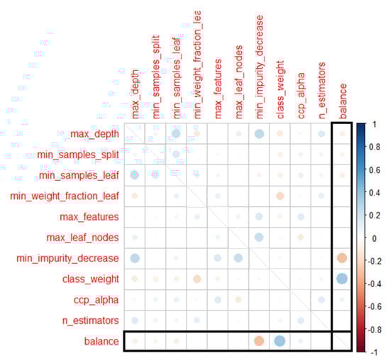
Figure 7.
Correlation matrix analysis of parameters.
Figure 8 plots the correlation between class weight and balance, which has positive correlation of 0.4. Figure 9 also plots the correlation between min_impurity_decrease and balance, which has negative correlation of 0.3. Both class_weight and min_impurity_decrease had weak correlation of less than 0.5.
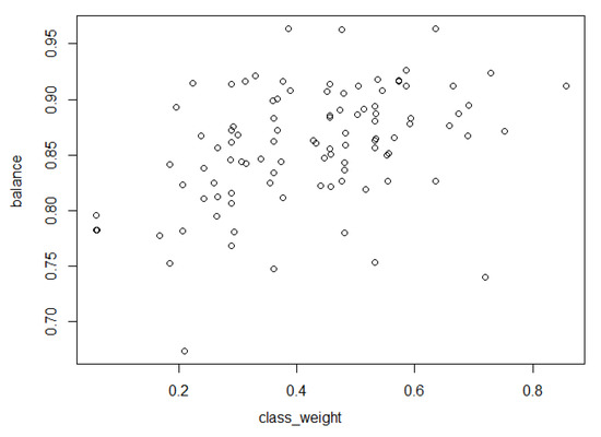
Figure 8.
Correlation between class_weight and balance.
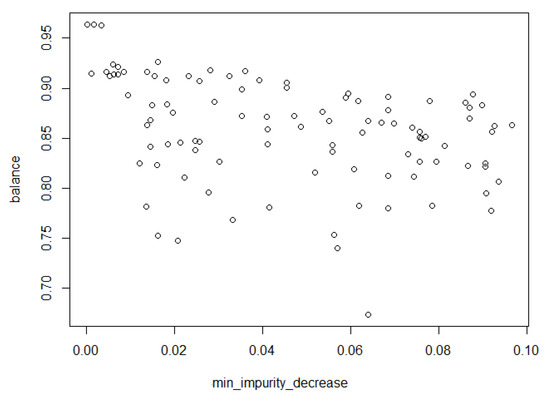
Figure 9.
Correlation between min_impurity_decrease and balance.
5.4. RQ4: How Does the Proposed Technique Perform in Open Source Software (OSS)?
In order to reinforce the rationale for our statement in RQ1, experiments were performed on 6 OSS datasets. We conducted additional experiments on the performance of our approach in open source projects with different characteristics and class imbalance ratios compared to the maritime domain. Table 9 shows the results of the experiment. The results are compared to the PD performed by Kamei et al. [7], and show that all PDs and balances were improved in all datasets with significant difference beyond large effect size. Note that we considered balance, increasing PD without worsening PF, in JIT-SDP. The best performance values are indicated in bold face and significant differences beyond medium size were underlined in the table.
Table 9.
Experimental results to answer RQ4.
6. Discussion
In this section, we discuss additional observations obtained through the result of the HS-based parameter optimization we performed.
The first is the relevance of the search space we designed. In our correlation matrix analysis conducted in RQ3, class_weight was an important parameter which had a weak positive correlation. On the other hand, since min_impurity has a negative correlation, it is a parameter that does not help to improve performance. Thus, it has become a guide to reducing prediction performance. We recommend that the search space can be effectively designed through the correlation analysis between the harmony and fitness values recorded in HM. In our experiment, changing class imbalanced ratio and class_weight of decision tree influenced the performance of prediction.
We also analyzed the impact of the performance by the presence or absence of a bagging classifier. We compared the performance results in RQ1 with the optimization using only the decision tree classifier. The results are summarized in Table 10. The best performance values are indicated in bold face and significant differences beyond medium size were underlined in the table. They showed that bagging increases PD and B, decreases PF, with significant differences. The bagging classifier is known as good meta-learner to prevent overfitting and reduce variance [42,43,44,45,46]. Catolino et al. [46] reported that they compare four base classifiers and four ensemble classification methods, but they did not find significant differences between the two. They mentioned that ensemble techniques should be able to improve the model performance with respect to single classifiers, but they concluded that ensemble techniques do not always guarantee better performance with respect to a single classifier in their work. In our experiment, the presence or absence of bagging had a significant effect on the performance improvement. Our dataset had unique characteristics that reflect practice in 2 maritime and 6 open source projects, and Catolino et al. had dataset characteristics that reflect practice in 14 mobile app projects. In the two studies, because contexts such as dataset, prediction model, and development environment are different from each other, the results seem to be different [47,48].
Table 10.
Effect of bagging classifier.
Finally, a comparison of performance improvement was made between maritime domain software and open source software. Both groups showed improvement in performance, but the baseline of maritime domain software already had high performance, so there was a limit to improve it. In our experiment in RQ1 varying class imbalance ratio, we observed significant performance improvement with high class imbalance datasets. On the other hand, in experiment RQ4, open source software showed a relatively high effect of performance improvement.
7. Threats to Validity
The generalization of the results is one of the main threats. Experimental results may differ if we use a dataset developed in a different environment than the dataset used in this article. Two datasets obtained from the maritime domain were used in the experiments. We chose HS-based parameter optimization in this work. There are widely used optimization algorithms, thus, the results may vary with different optimization algorithms with other classifiers.
8. Related Work
The prediction of just-in-time software defects helps to determine the buggy modules at such an earlier period and continuously once a change in software code is made [7,8,14]. The key benefits of JIT-SDP are that it is easy to anticipate buggy changes that are mapped to small parts of the code in order to save a lot of effort. It also makes it easier to identify who made the change, saving time identifying the developer who initiated the defect. Different granularity levels are categorized, such as software system, subsystem, component, package, file, class, method, or change in code. Since the smaller granularity will help practitioners lower their efforts, this contributes to cost-effectiveness. The prediction of defects at finer-grained levels has been researched to improve cost-effectiveness [7,14,49]. In many software defect datasets, class ratio of defect to non-defect is typically unbalanced. The unbalanced datasets result in poor prediction model [50]. The problem is called class imbalance. Class imbalance learning can improve performance by dealing with class imbalance at the instance-level or algorithm-level [29,51,52,53].
On the other hand, because researchers faced difficulties accessing industrial defect datasets because of data protection and privacy, only a few industrial applications of SDP were reported. Moreover, application of HS-based parameter optimization to both industry and JIT-SDP are the first case to the best of our knowledge.
Kamei et al. [7] proposed a just-in-time defect prediction technique with a large-scale empirical analysis that offers fine granularity. For the prediction model, a regression model was used, based on data derived from a total of 11 projects (i.e., six open source software and five commercial software). Fourteen change-level metrics grouped into five kinds were used: three kinds of code size, four kinds of diffusion, three kinds of history, three kinds of experience, and one kind of purpose. However, any parameter optimization were not considered. Balance was not considered as well. In this article, we also use the same 14 change level metrics, but the maritime industrial dataset was selected, experimented with HS-based parameter optimization with balanced fitness value.
Tosun et al. [54] addressed the implementation of SDP to a Turkish telecommunication firm as part of a software measurement initiative. The program was targeted to increase code quality and decrease both cost and defect rates. Using file-level code metrics, the naive Bayes model was built. Based on their project experience, they provided recommendations and best practice. However, parameter optimization was not considered in this program.
Catolino et al. [46] applied JIT-SDP to 14 open source projects in the mobile context with 14 change-level metrics. Two different groups of algorithm were compared: four base classifiers and four ensemble classifiers. In each category, the best performance result showed 49% f-measures with Naive and 54% f-measures with bagging, thus they found no significant differences between the two. Parameter optimization was not considered in this study.
Kang et al. [14] applied and performed experiments to explore the use of JIT-SDP in the maritime domain, for the first time. They demonstrated that SDP was feasible in the maritime domain and, based on their experimental findings, gave lessons learned and recommendations for practitioners. However, when they built the prediction model, except for the use of default values, parameter optimization for the various classification algorithms was not considered.
Ryu and Baik [55,56] applied HSA in multi-objective naïve Bayesian learning for cross-project defect prediction. The HSA searched the best weighted parameters, such as the class probability and the feature weights, based on three objectives. The three objects were PD, PF, and overall performance (e.g., balance). As a result, the proposed approaches showed a similar prediction performance compared to the within-project defect prediction model and produced a promising result. They applied HS optimization for file-level defect prediction. In this article, granularity was code change level, which has several of the merits mentioned above.
Tantithamthavorn et al. [34] applied automated parameter optimization on defect prediction models. Several studies pointed out that the classifiers underperformed since they used default parameters. Therefore, this paper studied the impact of parameter optimization on SDP with 18 datasets. As a result, the automated parameter optimization improved area under the curve (AUC) performance by up to forty percentage. This paper also highlighted the importance of exploring the search space when tuning parameter sensitive classification techniques, such as the decision tree.
Chen et al. [8] proposed multi-objective effort-aware just-in-time software defect prediction with six open source projects. The logistic regression model was optimized with coefficients such as decision variables and both accuracy and popt as fitness value. In this study, not parameters but coefficients of logistics were optimized. In this article, we used two industrial datasets in the maritime domain and six open source datasets together. The model we chose was bagging of decision trees inspiring the previous case study [14], and the performance index was balance considering class imbalance.
Through this literature review, we found that there is no case of parameter optimization of JIT-SDP based on HS, and there are no cases applied to the maritime domain.
9. Conclusions
The purpose of this study was to improve the performance of prediction applying HS-based parameter optimized JIT-SDP, HASPO, in maritime domain software, which is undergoing innovative transformations that require software technology. Using two real-world datasets collected from the domain, we obtained a better optimized model beyond the baseline of a previous case study [14] throughout various class imbalance ratio of datasets. Additional experiments with open source software showed a rather remarkably improved PD for all datasets despite the fact that we considered balance (i.e., maximization of PD and minimization of PF together) as performance index. Finally, we recommend that HASPO can be applied to JIT-SDP in the maritime domain software with high class imbalance ratio. Through this study, we found new possibilities in expanding our approach to open source projects. Our contribution is, to the best of our knowledge, that we apply HS-based parameter optimization with search space of decision tree and bagging classifier together with balanced fitness function in both JIT-SDP approach and the maritime domain for the first time.
In this paper, we consider metaheuristics for parameter optimization. To solve such optimization problems, metaheuristics are not the only method but a numerical optimization technique could be another solution [57,58,59]. Our research goal is to apply harmony search in this paper, and numerical optimization is not the scope of this research. In our future research, we will extend our work to perform comparative experiments using more optimization algorithms or mathematical programming with other classifiers, adding cost-aware fitness function, and improving generalization with datasets from other industries and open source software.
Author Contributions
J.K.: Conceptualization, planning, formal analysis, data curation, writing—original draft preparation. S.K.: writing—methodology and data visualization. D.R.: Conceptualization, writing—review and editing. J.B.: writing—review and editing, supervision, project administration. All authors have read and agreed to the published version of the manuscript.
Funding
This research was partly supported by National Research Foundation of Korea (NRF) and Institute of Information & Communications Technology Planning and Evaluation (No. NRF-2019R1G1A1005047 & No. IITP-2020-2020-0-01795).
Institutional Review Board Statement
Not applicable.
Informed Consent Statement
Not applicable.
Data Availability Statement
Not applicable.
Conflicts of Interest
The authors declare no conflict of interest.
Appendix A. Parameters of Decision Tree Classifier
Decision tree classifiers are commonly used supervised learning techniques for both classification and regression in order to construct prediction models by learning intuitive features in decision-making [42]. The key benefits of these are easy to grasp in the human context and to perceive by tree visualization. This needs little preparation of data and performs well. Table A1 shows the complete parameters of the decision tree classifier. We referenced all listings of parameters, descriptions and search spaces in Python scikit-learn library [39,40]. The selected column is our pre-designed values for each variable.
Table A1.
Whole parameters and selected search space for decision tree classifier [18].
Table A1.
Whole parameters and selected search space for decision tree classifier [18].
| Parameters | Description | Search Space | Selected |
|---|---|---|---|
| criterion | The measurement function of the quality of a split. Supported criteria are
| {“gini”, “entropy”}, default = “gini” | {“gini”, “entropy”} |
| splitter | The strategy of the split at each node. Supported strategies are
| {“best”, “random”}, default = “best” | {“best”, “random”} |
| max_depth | The maximum depth of the tree. If None, then expanded until all leaves are pure or until all leaves contain less than min_samples_split samples. | int, default = None | 10~20 |
| min_samples_split | The minimum number of samples required to split an internal node | int or float, default = 2 | 2~10 |
| min_samples_leaf | The minimum number of samples required to be at a leaf node | int or float, default = 1 | 1~10 |
| min_weight_fraction_leaf | The minimum weighted fraction of the sum total of weights required to be at a leaf node | float, default = 0.0 | 0~0.5 |
| max_features | The number of features to consider | int, float, default = None | 1~Max |
| random_state | Controls the randomness of the estimator | default = None | None |
| max_leaf_nodes | Grow a tree with max_leaf_nodes in best-first fashion. If None then unlimited number of leaf nodes | int, default = None | 1~100, 0: Unlimited |
| min_impurity_decrease | A node will be split if this split induces a decrease of the impurity greater than or equal to this value | float, default = 0.0 | 0.0~1.0 |
| min_impurity_split | Threshold for early stopping in tree growth. A node will split if its impurity is above the threshold, otherwise it is a leaf. | float, default = 0 | 0 |
| class_weight | Weights associated with each class | dict, list of dict or “balanced”, default = None | Weight within 0.0~1.0 for each class |
| ccp_alpha | Complexity parameter used for Minimal Cost-Complexity Pruning. No pruning is default | non-negative float, default = 0.0 | 0.0001~0.001 |
Appendix B. Parameters of Bagging Classifier
A bagging classifier is an ensemble classifier that fits the base classifiers on each of the original dataset subsets and then aggregates their predictions by either voting or averaging to create a final prediction. It can be used to reduce the variance of a black-box estimator, such as a decision tree, by integrating randomization into the creation process and then constructing an ensemble model [43]. The complete parameters of the bagging classifier are seen in Table A2. We referenced all listings of parameters, descriptions and search spaces in Python scikit-learn library [39,40]. The selected column is our pre-designed values for each variable.
Table A2.
Whole parameters and selected search space for bagging classifier [18].
Table A2.
Whole parameters and selected search space for bagging classifier [18].
| Parameters | Description | Search Space | Selected |
|---|---|---|---|
| base_estimator | The base estimator to fit on random subsets of the dataset. If None, then the base estimator is a decision tree. | object, default = None | default = None |
| n_estimators | The number of base estimators | int, default = 10 | 10~100 |
| max_samples | The number of samples from training set to train each base estimator | int or float, default = 1.0 | 0.0~1.0 |
| max_features | The number of features from training set to train each base estimator | int or float, default = 1.0 | 1~Max |
| bootstrap | Whether samples are drawn with replacement. If False, sampling without replacement is performed. | bool, default = True | 0,1 |
| bootstrap_features | Whether features are selected with replacement or not | bool, default = False | 0,1 |
| oob_score | Whether to use out-of-bag samples to estimate the generalization error. | bool, default = False | 0,1 |
| warm_start | Reuse the solution of the previous call to fit | bool, default = False | False |
| n_jobs | The number of jobs to run in parallel | int, default = None | None |
| random_state | Controls the random resampling of the original dataset | int or RandomState, default = None | None |
| verbose | Controls the verbosity when fitting and predicting | int, default = 0 | 0 |
Appendix C. Box Plots of Balance, Probability of Detection (PD), and Probability of False Alarm (PF)
Figure A1 depicted box plots of balance, PD, PF of HS-based parameter optimized JIT-SDP. Each group has five graphs which have three box plots for DT, DT+BG, DT+BG+HS. The order of graphs are A1, A2, through A5. The results showed balances and PDs of DT+BG+HS in most cases have the highest distribution while not worsening PF.


Figure A1.
Box plots of balance, probability of detection (PD), probability of false alarm (PF) of HS-based parameter optimized JIT-SDP.
Figure A1.
Box plots of balance, probability of detection (PD), probability of false alarm (PF) of HS-based parameter optimized JIT-SDP.


References
- Broy, M. Challenges in automotive software engineering. In Proceedings of the 28th International Conference on Software Engineering, Shanghai, China, 20–28 May 2006; pp. 33–42. [Google Scholar]
- Greenblatt, J.B.; Shaheen, S. Automated vehicles, on-demand mobility, and environmental impacts. Curr. Sustain. Renew. Energy Rep. 2015, 2, 74–81. [Google Scholar] [CrossRef]
- Kretschmann, L.; Burmeister, H.-C.; Jahn, C. Analyzing the economic benefit of unmanned autonomous ships: An exploratory cost-comparison between an autonomous and a conventional bulk carrier. Res. Transp. Bus. Manag. 2017, 25, 76–86. [Google Scholar] [CrossRef]
- Höyhtyä, M.; Huusko, J.; Kiviranta, M.; Solberg, K.; Rokka, J. Connectivity for autonomous ships: Architecture, use cases, and research challenges. In Proceedings of the 2017 International Conference on Information and Communication Technology Convergence (ICTC), Jeju, Korea, 18–20 October 2017; pp. 345–350. [Google Scholar]
- Abdel-Hamid, T.K. The economics of software quality assurance: A simulation-based case study. MIS Q. 1988, 12, 395–411. [Google Scholar] [CrossRef]
- Knight, J.C. Safety critical systems: Challenges and directions. In Proceedings of the 24th International Conference on Software Engineering, Orlando, FL, USA, 25 May 2002; pp. 547–550. [Google Scholar]
- Kamei, Y.; Shihab, E.; Adams, B.; Hassan, A.E.; Mockus, A.; Sinha, A.; Ubayashi, N. A large-scale empirical study of just-in-time quality assurance. IEEE Trans. Softw. Eng. 2012, 39, 757–773. [Google Scholar] [CrossRef]
- Chen, X.; Zhao, Y.; Wang, Q.; Yuan, Z. MULTI: Multi-objective effort-aware just-in-time software defect prediction. Inf. Softw. Technol. 2018, 93, 1–13. [Google Scholar] [CrossRef]
- Yang, X.; Lo, D.; Xia, X.; Zhang, Y.; Sun, J. Deep learning for just-in-time defect prediction. In Proceedings of the 2015 IEEE International Conference on Software Quality, Reliability and Security, Vancouver, BC, Canada, 3–5 August 2015; pp. 17–26. [Google Scholar]
- Jha, S.; Kumar, R.; Son, L.H.; Abdel-Basset, M.; Priyadarshini, I.; Sharma, R.; Long, H.V. Deep learning approach for software maintainability metrics prediction. IEEE Access 2019, 7, 61840–61855. [Google Scholar] [CrossRef]
- Shepperd, M.; Bowes, D.; Hall, T. Researcher bias: The use of machine learning in software defect prediction. IEEE Trans. Softw. Eng. 2014, 40, 603–616. [Google Scholar] [CrossRef]
- Singh, P.D.; Chug, A. Software defect prediction analysis using machine learning algorithms. In Proceedings of the 2017 7th International Conference on Cloud Computing, Data Science & Engineering-Confluence, Noida, India, 12–13 January 2017; pp. 775–781. [Google Scholar]
- Hoang, T.; Dam, H.K.; Kamei, Y.; Lo, D.; Ubayashi, N. DeepJIT: An end-to-end deep learning framework for just-in-time defect prediction. In Proceedings of the 2019 IEEE/ACM 16th International Conference on Mining Software Repositories (MSR), Montreal, QC, Canada, 25–31 May 2019; pp. 34–45. [Google Scholar]
- Kang, J.; Ryu, D.; Baik, J. Predicting just-in-time software defects to reduce post-release quality costs in the maritime industry. Softw. Pract. Exp. 2020. [Google Scholar] [CrossRef]
- Geem, Z.W.; Kim, J.H.; Loganathan, G.V. A new heuristic optimization algorithm: Harmony search. Simulation 2001, 76, 60–68. [Google Scholar] [CrossRef]
- Abualigah, L.; Diabat, A.; Geem, Z.W. A Comprehensive Survey of the Harmony Search Algorithm in Clustering Applications. Appl. Sci. 2020, 10, 3827. [Google Scholar] [CrossRef]
- Manjarres, D.; Landa-Torres, I.; Gil-Lopez, S.; Del Ser, J.; Bilbao, M.N.; Salcedo-Sanz, S.; Geem, Z.W. A survey on applications of the harmony search algorithm. Eng. Appl. Artif. Intell. 2013, 26, 1818–1831. [Google Scholar] [CrossRef]
- Mahdavi, M.; Fesanghary, M.; Damangir, E. An improved harmony search algorithm for solving optimization problems. Appl. Math. Comput. 2007, 188, 1567–1579. [Google Scholar] [CrossRef]
- Geem, Z.W. (Ed.) Music-Inspired Harmony Search Algorithm: Theory and Applications; Springer: Berlin/Heidelberg, Germany, 2009. [Google Scholar]
- Prajapati, A.; Geem, Z.W. Harmony Search-Based Approach for Multi-Objective Software Architecture Reconstruction. Mathematics 2020, 8, 1906. [Google Scholar] [CrossRef]
- Alsewari, A.A.; Kabir, M.N.; Zamli, K.Z.; Alaofi, K.S. Software product line test list generation based on harmony search algorithm with constraints support. Int. J. Adv. Comput. Sci. Appl. 2019, 10, 605–610. [Google Scholar] [CrossRef]
- Choudhary, A.; Baghel, A.S.; Sangwan, O.P. Efficient parameter estimation of software reliability growth models using harmony search. IET Softw. 2017, 11, 286–291. [Google Scholar] [CrossRef]
- Chhabra, J.K. Harmony search based remodularization for object-oriented software systems. Comput. Lang. Syst. Struct. 2017, 47, 153–169. [Google Scholar]
- Mao, C. Harmony search-based test data generation for branch coverage in software structural testing. Neural Comput. Appl. 2014, 25, 199–216. [Google Scholar] [CrossRef]
- Omran, M.G.H.; Mahdavi, M. Global-best harmony search. Appl. Math. Comput. 2008, 198, 643–656. [Google Scholar] [CrossRef]
- Geem, Z.W.; Sim, K.-B. Parameter-setting-free harmony search algorithm. Appl. Math. Comput. 2010, 217, 3881–3889. [Google Scholar] [CrossRef]
- Borg, M.; Svensson, O.; Berg, K.; Hansson, D. SZZ unleashed: An open implementation of the SZZ algorithm-featuring example usage in a study of just-in-time bug prediction for the Jenkins project. In Proceedings of the 3rd ACM SIGSOFT International Workshop on Machine Learning Techniques for Software Quality Evaluation, Tallinn, Estonia, 27 August 2019; pp. 7–12. [Google Scholar]
- Kotsiantis, S.B.; Kanellopoulos, D.; Pintelas, P.E. Data preprocessing for supervised leaning. Int. J. Comput. Sci. 2006, 1, 111–117. [Google Scholar]
- Chawla, N.V.; Bowyer, K.W.; Hall, L.O.; Kegelmeyer, W.P. SMOTE: Synthetic minority over-sampling technique. J. Artif. Intell. Res. 2002, 16, 321–357. [Google Scholar] [CrossRef]
- Öztürk, M.M. Comparing hyperparameter optimization in cross-and within-project defect prediction: A case study. Arab. J. Sci. Eng. 2019, 44, 3515–3530. [Google Scholar] [CrossRef]
- Yang, X.; Lo, D.; Xia, X.; Sun, J. TLEL: A two-layer ensemble learning approach for just-in-time defect prediction. Inf. Softw. Technol. 2017, 87, 206–220. [Google Scholar] [CrossRef]
- Huang, Q.; Xia, X.; Lo, D. Revisiting supervised and unsupervised models for effort-aware just-in-time defect prediction. Empir. Softw. Eng. 2019, 24, 2823–2862. [Google Scholar] [CrossRef]
- Kondo, M.; German, D.M.; Mizuno, O.; Choi, E.H. The impact of context metrics on just-in-time defect prediction. Empir. Softw. Eng. 2020, 25, 890–939. [Google Scholar] [CrossRef]
- Tantithamthavorn, C.; McIntosh, S.; Hassan, A.E.; Matsumoto, K. The impact of automated parameter optimization on defect prediction models. IEEE Trans. Softw. Eng. 2018, 45, 683–711. [Google Scholar] [CrossRef]
- Deng, W.; Chen, H.; Li, H. A novel hybrid intelligence algorithm for solving combinatorial optimization problems. J. Comput. Sci. Eng. 2014, 8, 199–206. [Google Scholar] [CrossRef]
- Zeng, X.; Martinez, T.R. Distribution-balanced stratified cross-validation for accuracy estimation. J. Exp. Theor. Artif. Intell. 2000, 12, 1–12. [Google Scholar] [CrossRef]
- Ryu, D.; Jang, J.; Baik, J. A hybrid instance selection using nearest-neighbor for cross-project defect prediction. J. Comput. Sci. Technol. 2015, 30, 969–980. [Google Scholar] [CrossRef]
- Shin, Y.; Meneely, A.; Williams, L.; Osborne, J.A. Evaluating complexity, code churn, and developer activity metrics as indicators of software vulnerabilities. IEEE Trans. Softw. Eng. 2010, 37, 772–787. [Google Scholar] [CrossRef]
- Pedregosa, F.; Varoquaux, G.; Gramfort, A.; Michel, V.; Thirion, B.; Grisel, O.; Prettenhofer, P.; Weiss, R.; Dubourg, V.; Vanderplas, J.; et al. Scikit-learn: Machine learning in Python. J. Mach. Learn. Res. 2011, 12, 2825–2830. [Google Scholar]
- Buitinck, L.; Louppe, G.; Blondel, M.; Pedregosa, F.; Mueller, A.; Grisel, O.; Niculae, V.; Prettenhofer, P.; Gramfort, A.; Grobler, J.; et al. API design for machine learning software: Experiences from the scikit-learn project. arXiv 2013, arXiv:1309.0238. [Google Scholar]
- Fairchild, G. pyHarmonySearch 1.4.3. Available online: https://pypi.org/project/pyHarmonySearch/ (accessed on 28 July 2020).
- Breiman, L. Pasting small votes for classification in large databases and on-line. Mach. Learn. 1999, 36, 85–103. [Google Scholar] [CrossRef]
- Breiman, L. Bagging predictors. Mach. Learn. 1996, 24, 123–140. [Google Scholar] [CrossRef]
- Ho, T. The random subspace method for constructing decision forests. Pattern Anal. Mach. Intell. 1998, 20, 832–844. [Google Scholar]
- Louppe, G.; Geurts, P. Ensembles on Random Patches. In Machine Learning and Knowledge Discovery in Databases; Springer: Berlin/Heidelberg, Germany, 2012; pp. 346–361. [Google Scholar]
- CATOLINO, Gemma; DI NUCCI, Dario; FERRUCCI, Filomena. Cross-project just-in-time bug prediction for mobile apps: An empirical assessment. In Proceedings of the 2019 IEEE/ACM 6th International Conference on Mobile Software Engineering and Systems (MOBILESoft), Montreal, QC, Canada, 25–26 May 2019; pp. 99–110. [Google Scholar]
- Maclin, R.; Opitz, D. An empirical evaluation of bagging and boosting. AAAI/IAAI 1997, 1997, 546–551. [Google Scholar]
- Bauer, E.; Kohavi, R. An empirical comparison of voting classification algorithms: Bagging, boosting, and variants. Mach. Learn. 1999, 36, 105–139. [Google Scholar] [CrossRef]
- Pascarella, L.; Palomba, F.; Bacchelli, A. Fine-grained just-in-time defect prediction. J. Syst. Softw. 2019, 150, 22–36. [Google Scholar] [CrossRef]
- Ryu, D.; Jang, J.; Baik, J. A transfer cost-sensitive boosting approach for cross-project defect prediction. Softw. Qual. J. 2017, 25, 235–272. [Google Scholar] [CrossRef]
- Elkan, C. The foundations of cost-sensitive learning. In Proceedings of the International Joint Conference on Artificial Intelligence, Seattle, WA, USA, 4–10 August 2001; Lawrence Erlbaum Associates Ltd.: Mahwah, NJ, USA, 2001; pp. 973–978. [Google Scholar]
- Krawczyk, B.; Woźniak, M.; Schaefer, G. Cost-sensitive decision tree ensembles for effective imbalanced classification. Appl. Soft Comput. 2014, 14, 554–562. [Google Scholar] [CrossRef]
- Lomax, S.; Vadera, S. A survey of cost-sensitive decision tree induction algorithms. ACM Comput. Surv. (CSUR) 2013, 45, 1–35. [Google Scholar] [CrossRef]
- Tosun, A.; Turhan, B.; Bener, A. Practical considerations in deploying ai for defect prediction: A case study within the turkish telecommunication industry. In Proceedings of the 5th International Conference on Predictor Models in Software Engineering, Vancouver, BC, Canada, 18–19 May 2009; pp. 1–9. [Google Scholar]
- Ryu, D.; Baik, J. Effective multi-objective naïve Bayes learning for cross-project defect prediction. Appl. Soft Comput. 2016, 49, 1062–1077. [Google Scholar] [CrossRef]
- Ryu, D.; Baik, J. Effective harmony search-based optimization of cost-sensitive boosting for improving the performance of cross-project defect prediction. KIPS Trans. Softw. Data Eng. 2018, 7, 77–90. [Google Scholar]
- Kvasov, D.E.; Mukhametzhanov, M.S. Metaheuristic vs. deterministic global optimization algorithms: The univariate case. Appl. Math. Comput. 2018, 318, 245–259. [Google Scholar] [CrossRef]
- Paulavičius, R.; Sergeyev, Y.D.; Kvasov, D.E.; Žilinskas, J. Globally-biased BIRECT algorithm with local accelerators for expensive global optimization. Expert Syst. Appl. 2020, 144, 113052. [Google Scholar] [CrossRef]
- Sergeyev, Y.D.; Kvasov, D.E.; Mukhametzhanov, M.S. On the efficiency of nature-inspired metaheuristics in expensive global optimization with limited budget. Sci. Rep. 2018, 8, 1–9. [Google Scholar] [CrossRef] [PubMed]


Publisher’s Note: MDPI stays neutral with regard to jurisdictional claims in published maps and institutional affiliations. |
© 2021 by the authors. Licensee MDPI, Basel, Switzerland. This article is an open access article distributed under the terms and conditions of the Creative Commons Attribution (CC BY) license (http://creativecommons.org/licenses/by/4.0/).