Long Short-Term Memory Network-Based Metaheuristic for Effective Electric Energy Consumption Prediction

Abstract

The Electric Energy Consumption Prediction (EECP) is a complex and important process in an intelligent energy management system and its importance has been increasing rapidly due to technological developments and human population growth. A reliable and accurate model for EECP is considered a key factor for an appropriate energy management policy. In recent periods, many artificial intelligence-based models have been developed to perform different simulation functions, engineering techniques, and optimal energy forecasting in order to predict future energy demands on the basis of historical data. In this article, a new metaheuristic based on a Long Short-Term Memory (LSTM) network model is proposed for an effective EECP. After collecting data sequences from the Individual Household Electric Power Consumption (IHEPC) dataset and Appliances Load Prediction (AEP) dataset, data refinement is accomplished using min-max and standard transformation methods. Then, the LSTM network with Butterfly Optimization Algorithm (BOA) is developed for EECP. In this article, the BOA is used to select optimal hyperparametric values which precisely describe the EEC patterns and discover the time series dynamics in the energy domain. This extensive experiment conducted on the IHEPC and AEP datasets shows that the proposed model obtains a minimum error rate relative to the existing models.

1. Introduction

In recent decades, the demand for electricity has been rising on a global scale due to the massive growth of electronic markets [1], the development of electrical vehicles [2], the use of heavy machinery equipment (e.g., line excavators, pile boring machines) [3], technological advancements, and rapid population growth [4,5]. As a result, accurate electric load forecasting has greater importance in the field of power system planning [6]. An underestimation reduces the reliability of the power system, while overestimation wastes energy resources and effectively enhances operational costs [7]. Therefore, a precise electric load forecasting system is necessary for power systems, the electrical load series being affected by several influencing factors [8]. Currently, several electrical load forecasting models are being developed. The models fall into two categories: multi-factor forecasting models and time series forecasting models [9]. The time series forecasting models are quicker and easier in EECP compared to the multi-factor forecasting models. Numerous non-objective factors and electric load series are affected in practical applications, and it is difficult to control these with multi-factor forecasting models [10,11,12]. Hence, the multi-factor forecasting models simply evaluate the relations between forecasting variables and influencing factors [13,14,15]. In this research, a novel metaheuristic based on an LSTM model is developed to generate a more effective EECP. The main contributions are specified below:

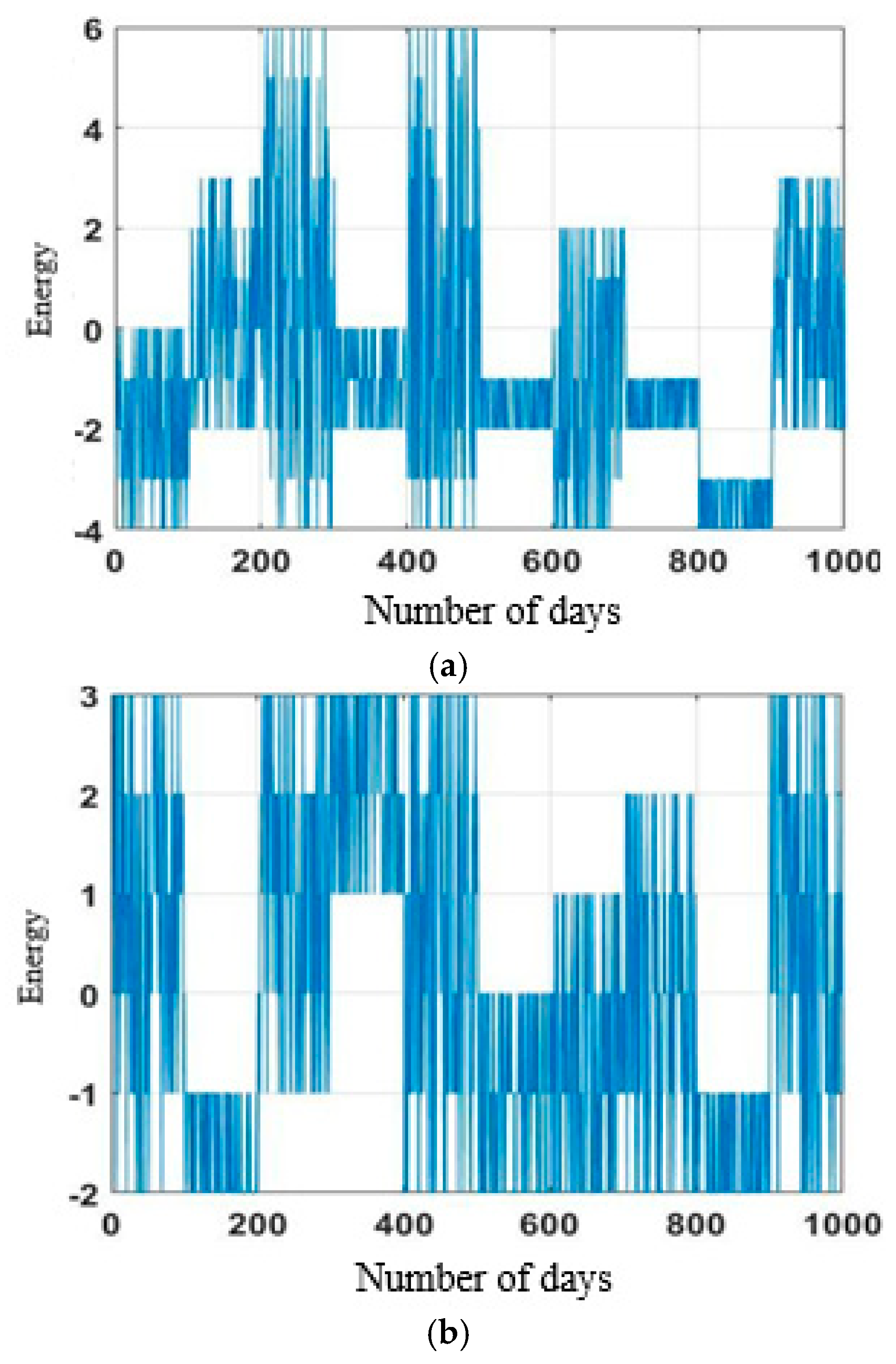
• Input data sequences are collected from IHEPC and AEP datasets, and data refinement is accomplished using min-max along with standard transformation methods in order to eliminate redundant, missing, and outlier variables.
• Next, the EECP is generated using the proposed metaheuristic based on the LSTM model. The proposed model superiorly handles the irregular tendencies of energy consumption relative to other deep learning models and conventional LSTM networks.
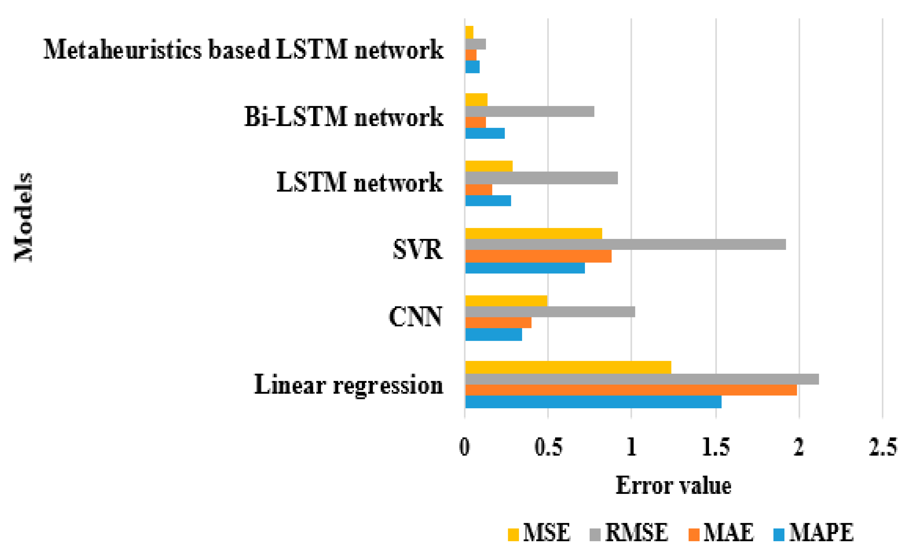
• The effectiveness of the proposed metaheuristic based on the LSTM model is evaluated in terms of mean squared error (MSE), root MSE (RMSE), mean absolute error (MAE) and mean absolute percentage error (MAPE) on both IHEPC and AEP datasets.

This article is structured as follows. Previous existing research studies on the topic of EECP are reviewed in Section 2. The mathematical explanations of the proposed metaheuristic based on the LSTM model and a quantitative study including experimental results are specified in Section 3 and Section 4, respectively. Finally, the conclusion of this work is stated in Section 5.

2. Related Works

In this section, previous works in the area are reviewed in order to justify the contribution of the proposal and the selection of strategies considered for comparison in the experimental section.

Le et al. [16] combined a Bidirectional Long Short-Term Memory (Bi-LSTM) network and a Convolutional Neural Network (CNN) to forecast household EEC. Firstly, the CNN was employed to extract the discriminative feature values from the IHEPC dataset and then the Bi-LSTM network was used to make predictions. Ishaq et al. [17] introduced a new ensemble-based deep learning model to forecast and predict energy consumption and demands. Initially, data pre-processing was performed using transformation, normalization, and cleaning techniques, and then the pre-processed data were fed into the ensemble model, the CNN and Bi-LSTM network extracting discriminative feature values. In this work, an active learning concept was created on the basis of the moving window to improve and ensure the prediction performance of the presented model. In the resulting phase, the effectiveness of the presented model was tested on a Korean commercial building dataset in light of MAPE, RMSE, MAE, and MSE values. Lin et al. [18] integrated an Extreme Learning Machine (ELM) and Variational Mode Decomposition (VMD) techniques for electrical load forecasting. Firstly, the VMD technique was employed to transform the collected electric load series into components with dissimilar frequencies, which helps to eliminate fluctuation properties and enhances the overall accuracy of prediction. Finally, EEC forecasting was carried out utilizing ELM with a differential evolution algorithm.

Xu et al. [19] combined a Deep Belief Network (DBN) and linear regression techniques to predict time series data. In this study, the linear regression technique captures the non-linear and linear behaviors of the time series data. Initially, the linear regression technique was used to obtain the residuals between input and predicted data, and then the residuals were fed into the DBN for the final forecasting. In the time series forecasting, the DBN significantly extracts the features between self-organization properties and layers. Maldonado et al. [20] applied Support Vector Regression (SVR) to the time series data for electric load forecasting. The SVR technique successfully modelled the nonlinear relation between the target variables and the exogenous covariates. Wan et al. [21] developed a new multivariate temporal convolutional network for time series prediction that has been extensively used in applications such as transportation, finance, aerology, and power/energy. In the time series data forecasting, the presented convolution network superiorly enhanced the results of EECP. Further, this study concentrates on the trade-off between prediction accuracy and implementation complexity. Bouktif et al. [22] combined a genetic algorithm and a Particle Swarm Optimization (PSO) algorithm to select optimal hyperparameters in LSTM for an effective EECP.

Qiu et al. [23] introduced an oblique random forest classifier for time series forecasting. In the developed classification technique, every node of the decision tree was replaced by the optimal feature-based orthogonal classifier. Additionally, the least square classification technique was used to perform feature partition. The efficiency of the oblique random forest classifier was investigated using five electricity load time series datasets and eight general time series datasets. Further, Kuo and Huang [24] presented a new deep learning network for short term energy load forecasting. The obtained results showed that the deep-energy model was robust and had a strong generalization ability in data series forecasting. Similarly, Qiu et al. [25] combined DBN and empirical mode decomposition for electricity load demand forecasting. Initially, the acquired data series were decomposed into several Intrinsic Mode Functions (IMFs). Further, the DBN was applied to model each of the extracted IMFs for accurate prediction. Pham et al. [26] implemented a random forest classifier to forecast household short-term energy consumption. The effectiveness of the random forest classifier was tested on five one-year datasets. The evaluation outcome showed that the presented random forest classifier obtained better predictive accuracy by means of MAE.

Galicia et al. [27] introduced an ensemble classifier by combining random forest, gradient boosted trees and decision trees to forecast big data time series. The evaluation results showed that the developed ensemble classifier performed well in time series data prediction compared to other models and individual ensemble models. Khairalla et al. [28] presented a new stacking multi-learning ensemble model for forecasting time series data. The presented model includes three main techniques—SVR, linear regression, and a backpropagation neural network—and the presented ensemble model comprises four major steps: integration, pruning, generation, and ensemble prediction tasks. Jallal et al. [29] introduced a hybrid model that integrates a firefly algorithm and an Adaptive Neuro Fuzzy Inference System (ANFIS) classifier for EECP, though the improved search space diversification in the presented model enhances its predictive accuracy. Bandara et al. [30] introduced a new LSTM Multi-Seasonal Net (LSTM-MSNet) for time series forecasting with multiple seasonal patterns. The evaluation outcome showed that the presented LSTM-MSNet model achieved better computational time and prediction accuracy compared to existing systems. Abbasimehr and Paki [31] combined multi-head attention and LSTM networks to predict the time series data precisely. Sajjad et al. [32] initially used min-max and standard transformation techniques to eliminate outlier, redundant, and null values from the IHEPC and AEP datasets. Then, EECP was accomplished using CNN with a Gated Recurrent Units (GRUs) model. The experimental evaluation showed that the presented model obtained a significant performance in EECP by means of MAE, RMSE, and MSE.

Khan et al. [33] combined a Bi-LSTM network and dilated CNN to predict power consumption in local energy systems. As can be seen in the resulting phase, the presented model effectively predicts multiple step power consumption that includes monthly, weekly, daily, and hourly outputs. Khan et al. [34] has integrated multilayer bi-directional GRU and CNNs for household electricity consumption prediction. The effectiveness of the presented model was evaluated in terms of MAE, RMSE, and MSE on the IHEPC and AEP datasets.

Nowadays, artificial intelligence techniques are applied more in the application of EECP because of its reliability and high performance results. The artificial intelligence-based techniques, such as CNN, GRU, multi head attentions, ANFIS, and the ensemble schemes, are extensively applied for energy forecasting and time series issues. The GRU technique obtained a better outcome in EECP related to conventional techniques, but it is ineffective in handling long-term time series data sequences, and it is also historically dependent. In addition, the aforementioned techniques failed in long-term consequence forecasting and includes vanishing gradient issues [35]. To overcome the above stated concerns, a new metaheuristic based on the LSTM network is proposed in this article to predict and handle the short-term and long-term dependencies in energy forecasting.

3. Proposal

The proposed metaheuristics based on the LSTM network includes three major phases in EECP, namely, data collection (AEP and IHEPC datasets), data refinement (min-max transformation and standard transformation methods) and consumption prediction (using metaheuristics based on the LSTM network). The flow-diagram of the proposed model is specified in Figure 1.

Figure 1. Flow-diagram of the proposed model.

3.1. Dataset Description

In the household EECP application, the effectiveness of the proposed metaheuristics-based LSTM network is validated with AEP and IHEPC datasets. The AEP dataset contains 29 parameters related to appliances’ energy consumption, lights, and weather information (pressure, temperature, dew point, humidity, and wind speed), which are statistically depicted in Table 1. The AEP dataset includes data for four and half months of a residential house at a ten-minute resolution. In the AEP dataset, the data are recorded from the outdoor and indoor environments using a wireless sensor network, the outdoor data being acquired from a near-by airport [36]. The residential house contains one outdoor temperature sensor, nine indoor temperature sensors, and nine humidity sensors; one sensor is placed in the outdoor environment and seven humidity sensors are placed in the indoor environment. The humidity, outdoor pressure, temperature, dew point, and visibility are recorded at the near-by airport. The statistical information about the AEP dataset is depicted in Table 1.

Table 1. Statistical information about the AEP dataset.

Attributes	Information	Units
Dew point	Outside dew point recorded from Chievres Weather Station (CWS)	C
Visibility	Outside visibility recorded from CWS	Km
Wind speed	Outside wind speed recorded from CWS	m/s
Rho	Outside humidity recorded from CWS	%
Pressure	Outside pressure recorded from CWS	Mm Hg
To	Outside temperature recorded from CWS	C
RH1	Humidity of parents’ room	%
T1	Temperature of parents’ room	C
RH2	Humidity of teenager’s room	%
T2	Temperature of teenager’s room	C
RH3	Humidity of ironing room	%
T3	Temperature of ironing room	C
RH4	Outside humidity of building	%
T4	Outside temperature of building	C
RH5	Humidity of bathroom	%
T5	Temperature of bathroom	C
RH6	Humidity of office room	%
T6	Temperature of office room	C
RH7	Humidity of laundry room	%
T7	Temperature of laundry room	C
RH8	Humidity of living room	%
T8	Temperature of living room	C
RH9	Humidity of kitchen	%
T9	Temperature of kitchen	C
Light	Total energy consumption by lights	Watt-hour (Wh)
Appliances	Total energy consumption by appliances	Wh

In addition, the IHEPC dataset comprises of 2,075,259 instances, which are recorded from a residential house in France for five years (From December 2006 to November 2010) [37]. The IHEPC dataset includes nine attributes like voltage, minute, global intensity, month, global active power, year, global reactive power, day and hour. Three more variables are acquired from energy sensors: sub metering 1, 2, and 3 with proper meaning. The statistical information about IHEPC dataset is represented Table 2. The data samples of AEP and IHEPC datasets are graphically presented in the Figure 2.

Table 2. Statistical information about IHEPC dataset.

Attributes	Information
Sub metering 1	Energy utilized in kitchen (Wh)
Sub metering 2	Energy utilized in laundry room (Wh)
Sub metering 3	Energy utilized by water heater (Wh)
Date	dd/mm/yyyy
Time	hh:mm:ss
Voltage	Minute averaged voltage of household (volt)
Global reactive voltage	Minute averaged global reactive voltage of household (kilowatt (kW))
Global active voltage	Minute averaged global active voltage of household (kW)
Global intensity	Minute averaged global intensity of household (ampere)

Figure 2. Data samples of (a) the AEP dataset and (b) the IHEPC dataset.

3.2. Data Refinement

After the acquisition of data from the AEP and IHEPC datasets, data refinement is performed to eliminate missing and outlier variables and to normalize the acquired data. In the AEP dataset, a standard transformation technique is employed for converting the acquired data into a particular range. In the AEP dataset, the feature vectors range lies between 0 and 800, and by using the standard transformation technique the feature vectors range is transformed into −4 and −6. The mathematical expression of the standard transformation technique is defined in Equation (1):

$$T_{standard}=\left(X-U\right)/S$$

(1)

where $S$ indicates standard deviation, $X$ denotes actual acquired data, and $U$ represents the mean. In addition, the IHEPC dataset comprises redundant, outlier, and null values, so a min-max scalar is applied to eliminate non-significant values and to bring the feature vectors into a particular range of values. In the IHEPC dataset, the feature vectors range lies between 0 to 250, and by using the min-max transformation technique, the feature vectors range is transformed into −2 and −3. The mathematical expression of the min-max transformation technique is defined in Equation (2):

$$T_{min-max}=\frac{X-X_{min}}{X_{max}-X_{min}}$$

(2)

where $X_{max}$ and $X_{min}$ indicates maximum and minimum values of the IHEPC dataset. A total of 2890 and 25,980 missing values are eliminated in the AEP and IHEPC datasets utilizing the pre-processing techniques. The refined data samples of AEP dataset and IHEPC dataset are presented in Figure 3.

Figure 3. Refined data samples of (a) the AEP dataset and (b) the IHEPC dataset.

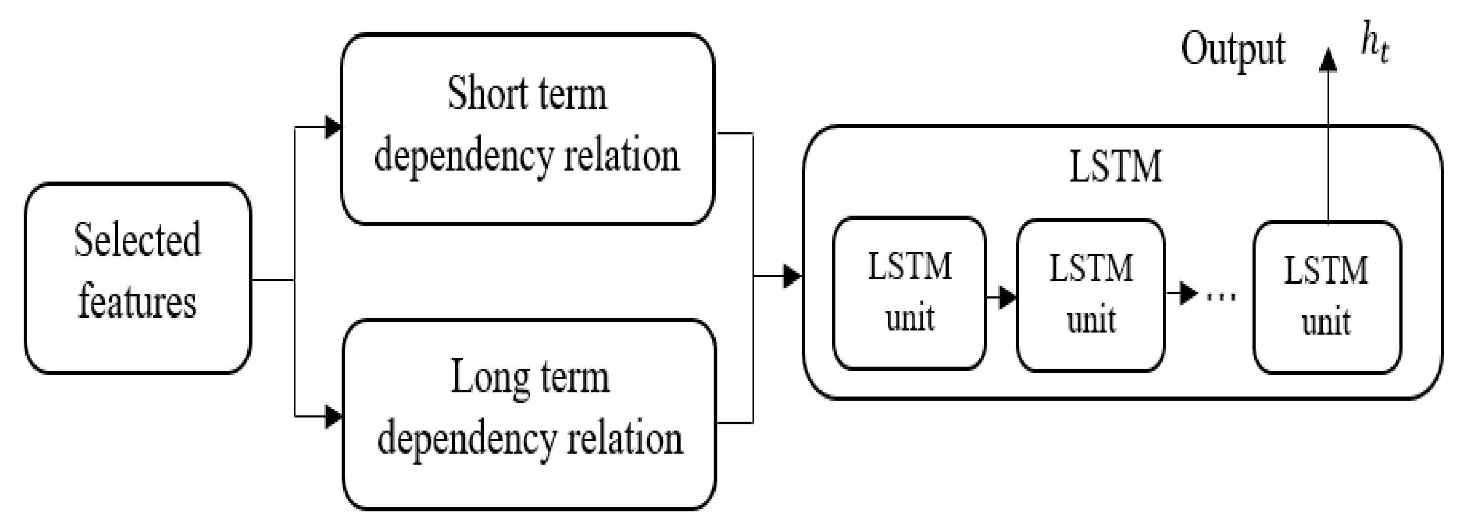
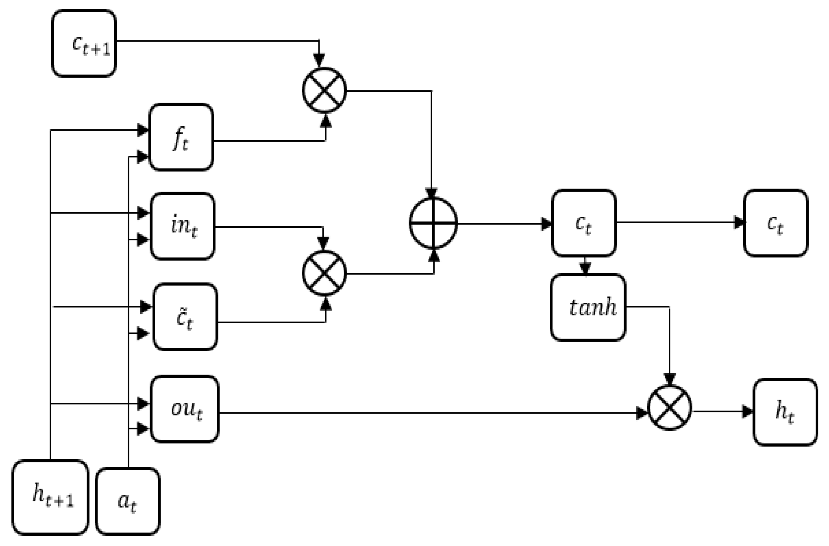
3.3. Energy Consumption Prediction

After refining the acquired data, the EECP is accomplished using the metaheuristics-based LSTM network. The LSTM network is an extension of a Recurrent Neural Network (RNN). The RNN has numerous problems, such as short-term memory and vanishing gradient issues, when it processes large data sequences [38]. In addition, the RNN is inappropriate for larger data sequences because it removes the important information from the input data. In the RNN model, the gradient updates the weights during back propagation, where sometimes it reduced highly and the initial layers get low gradient and stops further learning. To tackle these issues, the LSTM network was developed by Hochreiter [39]. The LSTM network overcomes the issues of RNNs by replacing hidden layers with memory cells for modelling long-term dependencies. The LSTM network includes dissimilar gates, such as a forget gate, input gate, and output gate, along with activation functions for learning time-based relations. The LSTM network and the individual LSTM unit are graphically depicted in Figure 4 and Figure 5.

Figure 4. Graphical presentation of the LSTM network.

Figure 5. Graphical presentation of the LSTM unit.

The mathematical expressions of the input gate $i{n}_t$, forget gate $f_t$, cell $c_t$, and output gate $o{u}_t$ are defined in Equations (3)–(6):

$$i{n}_t=\sigma \left(W_{inh}{h}_{t-1}+W_{ina}{a}_t+b_{in}\right)$$

(3)

$$f_t=\sigma \left(W_{fh}{h}_{t-1}+W_{fa}{a}_t+b_f\right)$$

(4)

$$c_t=f_t\odot c_{t-1}+i{n}_t\odot \tan \mathrm{h}\left(W_{ch}{h}_{t-1}+W_{ca}{a}_t+b_c\right)$$

(5)

$$o{u}_t=\sigma \left(W_{ouh}{h}_{t-1}+W_{oua}{a}_t+b_{ou}\right)$$

(6)

where $t$ represents different time steps, $a_t=A\left[t, .\right]\in {ℝ}^F$ represents temporal quasi-periodic feature vectors, $tanh (.)$ denotes a hyperbolic tangent function, $\sigma (.)$ states a sigmoid function, and $W$ and $b$ work coefficients. The output of the LSTM unit $h_{t-1}$ is mathematically specified in Equation (7), and it is graphically presented in Figure 5:

$$h_t=o{u}_t\odot \tanh \left(c_t\right)$$

(7)

The cell state $\left\{c_t\left|t=1,2,..T\right|\right\}$ learns the necessary information from $a_t$ on the basis of the dependency relationship during the training and testing mechanism. Finally, the extracted feature vectors are specified by the last LSTM unit output $h_T$. The hyperparametric values selected using BOA for the LSTM network are listed as follows: the number of sequences are 2 and 3, the sequence length is from 7 to 12, the minimum batch size is 20, the learning rate is 0.001, the number of the LSTM unit is 55, the maximum epoch is 120, and the gradient threshold value is 1. The BOA is a popular metaheuristic algorithm, which mimics the butterfly’s behavior in foraging and mating. Biologically, butterflies are well adapted for foraging, possessing sense receptors that allow them to detect the presence of food. The sense receptors are known as chemoreceptors and are dispersed over several of the butterfly’s body parts, such as the antennae, palps, legs, etc. In the BOA, the butterfly is assumed as a search agent to perform optimization and the sensing process depends on three parameters such as sensory modality, power exponent and stimulus intensity. If the butterfly is incapable of sensing the fragrance, then it moves randomly in the local search space [40].

Whereas, the sensory modality is in the form of light, sound, temperature, pressure, smell, etc. and it is processed by the stimulus. In the BOA, the magnitude of the physical stimulus is denoted as $M$ and it is associated with the fitness of butterfly with greater fragrance value in the local search space. In the BOA, the searching phenomenon depends on two important issues: formulation of fragrance $q$ and variations of physical stimulus $M$. For simplicity purpose, the stimulus intensity $M$ is related with encoded-objective-function. Hence, $q$ is relative and is sensed by other butterflies in the local search space. In the BOA, the fragrance is considered as a function of the stimulus, which is mathematically defined in Equation (8):

$$q_i=z{l}^d$$

(8)

where $z$ denotes the sensory modality, $l$ the perceived magnitude of fragrance, $M$ the stimulus intensity and $d$ indicates the power exponent. The BOA consists of two essential phases: a local and a global search phase. In the global search phase, the butterfly identifies the fitness solution that is determined in Equation (9):

$$x_i^{t+1}=x_i^t+\left(levy \left(\lambda \right)\times g^{\ast }-x_i^t\right)\times q_i$$

(9)

where $x_i^t$ indicates the vector $x_i$ of the $i\mathrm{th}$ butterfly, $t$ represents iteration, $g^{\ast }$ the present best solution, $q_i$ states fragrance of the butterfly and $levy \left(\lambda \right)$ denotes a random number that ranges between 0 and 1. The general formula for calculating the local search phase is given in Equation (10):

$$x_i^{t+1}=x_i^t+\left(levy \left(\lambda \right)\times x_k^t-x_i^t\right)\times q_i$$

(10)

where $x_k^t \mathrm{and} x_i^t$ are the kth/ith butterflies from the solution. If $x_k^t \mathrm{and} x_i^t$ belongs to the same flight, Equation (10) performs a local random walk. The flowchart of the BOA is depicted in Figure 6.

Figure 6. Flowchart of the BOA.

In this scenario, the iteration phase is continued until the stopping criteria is not matched. The pseudocode of the BOA is represented as follows (Algorithm 1):

Algorithm 1 Pseudocode of BOA

Objective function $q\left(x\right), x_i \left(i=1,2,\dots .n\right)$ Initialize butterfly population In the initial population, best solution is identified Determine the probability of switch $P$ While stopping criteria is not encountered do For every butterfly do Draw $rand$ Find butterfly fragrance utilizing Equation (8) If $rand<P$ then Accomplish global search utilizing Equation (9) Else Accomplish local search utilizing Equation (10) End if Calculate the new solutions Update the best solutions End for Identify the present better solution End while Output: Better solution is obtained

4. Experimental Results

In the EECP application, the proposed metaheuristic based on the LSTM network is simulated using a Python software environment on a computer with 64 GB random access memory, a TITAN graphics processing unit with Intel core i7 processor and Ubuntu operating system. The effectiveness of the proposed metaheuristic based on the LSTM network in EECP is validated by comparing its performance with benchmark models, such as a Bi-LSTM with CNN [16], an ensemble-based deep learning model [17], a CNN with GRU model [32], a Bi-LSTM with dilated CNN [33], and multilayer bi-directional GRU with CNN [34] on the AEP and IHEPC datasets. In this research, the experiment is conducted using four performance measures, MAPE, MAE, RMSE, and MSE, for time series data prediction. The MAPE is used to estimate the prediction accuracy of the proposed metaheuristic based on the LSTM network. The MAPE performance measure represents accuracy in percentage, as stated in Equation (11):

$$\mathrm{MAPE}=\frac{1}{n}{\displaystyle \sum }_1^n|\frac{y-\widehat{y}}{y}|$$

(11)

The MAE is used to estimate the average magnitude of the error between actual and predicted values by ignoring their direction. The MSE is used to determine the mean disparity between actual and predicted values. The mathematical expressions of MAE and MSE are stated in the Equations (12) and (13). Correspondingly, the RMSE is used to find the dissimilarity between the actual and predicted values, and then the mean of the square errors is computed. Lastly, the square root of the mean values is calculated, where the mathematical expression of RMSE is stated in Equation (14):

$$\mathrm{MAE}=\frac{1}{n}{\displaystyle \sum }_1^n|y-\widehat{y}|$$

(12)

$$\mathrm{MSE}=\frac{1}{n}{\displaystyle \sum }_1^n{\left(y-\widehat{y}\right)}^2$$

(13)

$$\mathrm{RMSE}=\sqrt{\frac{1}{n}{\displaystyle \sum }_1^n{\left(y-\widehat{y}\right)}^2}$$

(14)

where $n$ represents the number of instances, $y$ the actual value and $\widehat{y}$ the prediction value.

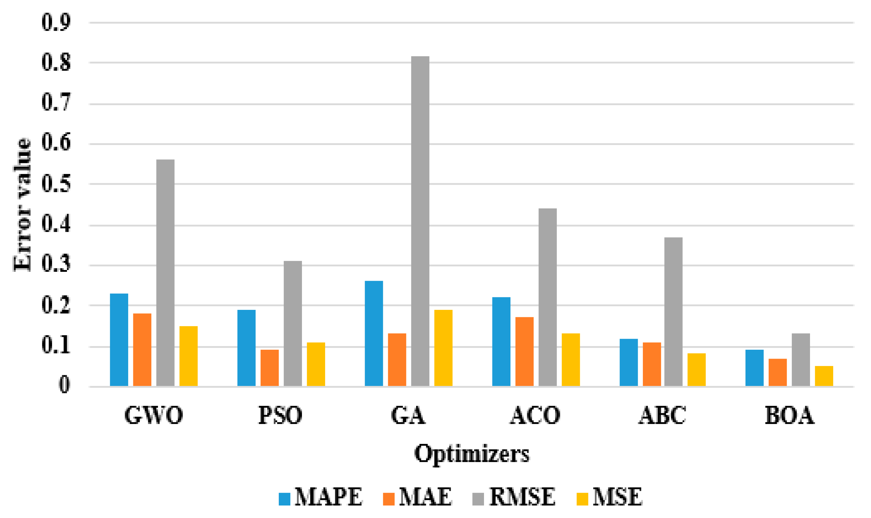
4.1. Quantitative Study on AEP Dataset

In this scenario, an extensive experiment is conducted on the AEP dataset to evaluate and validate the proposed metaheuristic based on the LSTM network’s effectiveness and robustness for real-world issues. The refined AEP dataset is split into a 20:80% ratio for the proposed model’s testing and training. The proposed metaheuristic based on the LSTM network utilizes 20% of data during testing and 80% of data during training. As seen in Table 3, the proposed metaheuristic based on the LSTM network obtained results closely related to the native properties of energy and the actual consumed energy level. By inspecting Table 3, the proposed model achieved effective results compared to other existing models, such as linear regression, CNN, SVR, the LSTM network and the Bi-LSTM network in light of MAPE, MAE, RMSE and MSE. Hence, the irregular tendencies of energy consumption are easily and effectively handled by the proposed metaheuristic based on the LSTM network. Hence, the proposed model attained a minimum MAPE of 0.09, an MAE of 0.07, an RMSE of 0.13, and an MSE of 0.05. In addition to this, the proposed model reduces prediction time by almost 30% compared to other models for the AEP dataset. A graphical presentation of the experimental models for the AEP dataset is depicted in Figure 7.

Table 3. Performance of the experimental models on the AEP dataset.

Models	MAPE	MAE	RMSE	MSE	Predicting Time (s)
Linear regression	1.54	1.99	2.12	1.24	38
CNN	0.34	0.40	1.02	0.49	29
SVR	0.72	0.88	1.92	0.82	49
LSTM network	0.28	0.17	0.92	0.29	21
Bi-LSTM network	0.24	0.13	0.78	0.14	18
Metaheuristic based on the LSTM network	0.09	0.07	0.13	0.05	12

Figure 7. Graphical presentation of the experimental models for the AEP dataset.

In Table 4, the hyperparameter selection in the LSTM network is carried out with dissimilar optimization techniques, such as BOA, Grey Wolf Optimizer (GWO), Particle Swarm Optimizer (PSO), Genetic Algorithm (GA), Ant Colony Optimizer (ACO), and Artificial Bee Colony (ABC), and the performance validation is done using four metrics, namely, MAPE, MAE, RMSE, and MSE on the AEP dataset. As evident from Table 4, the combination of the LSTM network with BOA obtained an MAPE of 0.09, an MAE of 0.07, an RMSE of 0.13, and an MSE of 0.05, which are minimal compared to other optimization techniques. Due to naive selection of the hyperparametric values and the noisy electric data, the LSTM network obtained unacceptable forecasting results. An optimal LSTM network configuration is therefore needed to discover the time series dynamics in the energy domain and to describe the electric consumption pattern precisely. In this article, a metaheuristic-based BOA is applied to identify the optimal hyperparametric values of the LSTM network in the EEC domain. The BOA effectively learns the hyper parameters of the LSTM network to forecast energy consumption. Graphical presentation of dissimilar hyperparameter optimizers in the LSTM network on the AEP dataset is depicted in Figure 8.

Table 4. Performance of the dissimilar hyperparameter optimizers in the LSTM network on the AEP dataset.

LSTM Network
Optimizers	MAPE	MAE	RMSE	MSE	Predicting Time (s)
GWO	0.23	0.18	0.56	0.15	30
PSO	0.19	0.09	0.31	0.11	43
GA	0.26	0.13	0.82	0.19	64
ACO	0.22	0.17	0.44	0.13	29
ABC	0.12	0.11	0.37	0.08	25
BOA	0.09	0.07	0.13	0.05	12

Figure 8. Graphical presentation of the dissimilar hyperparameter optimizers in the LSTM network on the AEP dataset.

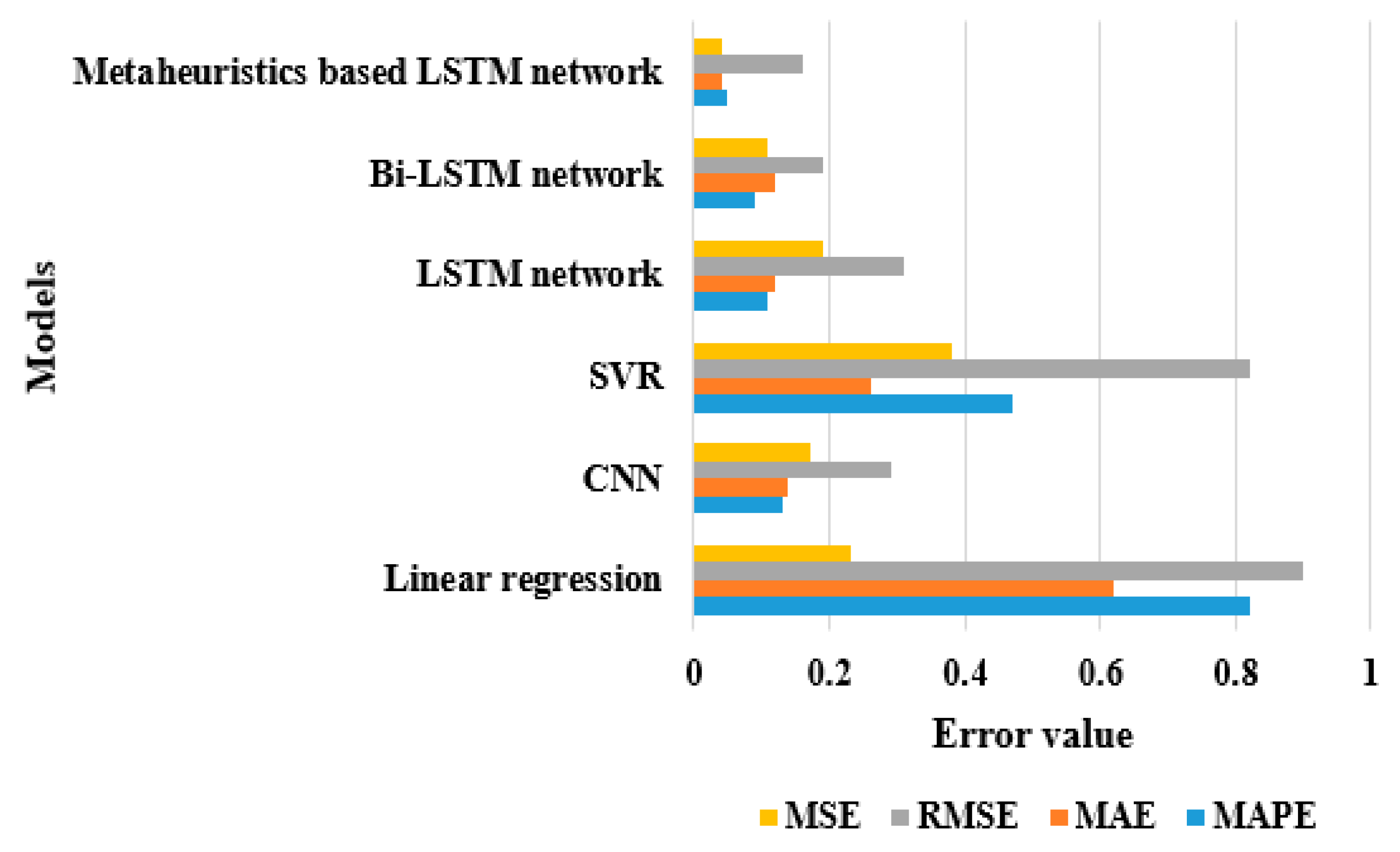
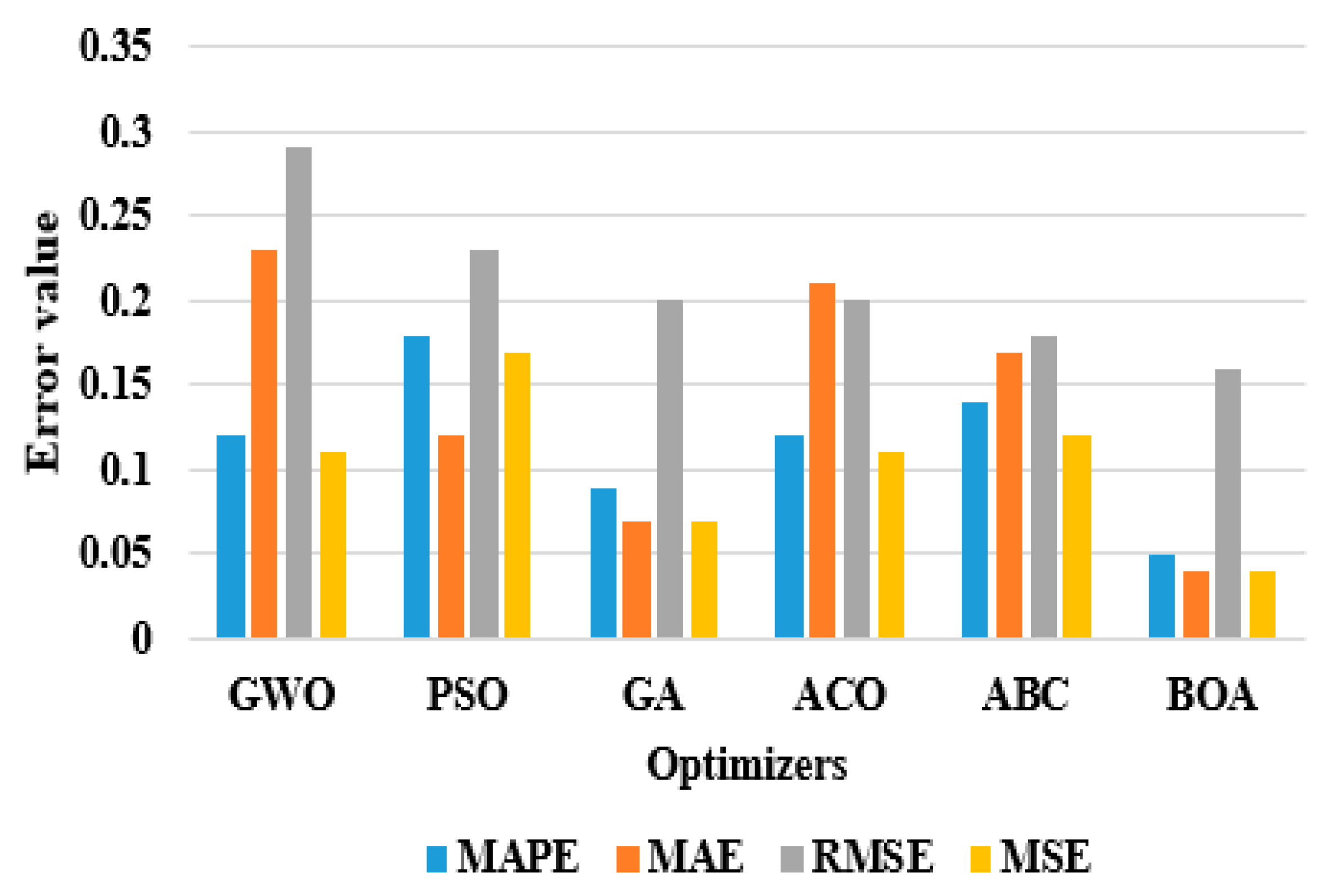
4.2. Quantitative Study on IHEPC Dataset

Table 5 represents the extensive experiment conducted on the IHEPC dataset to evaluate the efficiency of the proposed metaheuristic based on the LSTM network by means of MAPE, MAE, RMSE, and MSE. The proposed metaheuristic based on the LSTM network obtained a minimum MAPE of 0.05, an MAE of 0.04, an RMSE of 0.16, and an MSE of 0.04, which are effective compared to other experimental models, such as linear regression, CNN, SVR, the LSTM network, and the Bi-LSTM network on the IHEPC database. In addition, the prediction time of metaheuristic based on LSTM network is 25% minimum compared to other experimental models. In this research, the metaheuristic based on the LSTM network superiorly handles the complex time series patterns and moderates the error value at every interval related to the other experimental models. Graphical presentation of the experimental models for the IHEPC dataset is depicted in Figure 9.

Table 5. Performance of the experimental models on IHEPC dataset.

Models	MAPE	MAE	RMSE	MSE	Predicting Time (s)
Linear regression	0.82	0.62	0.90	0.23	34
CNN	0.13	0.14	0.29	0.17	22
SVR	0.47	0.26	0.82	0.38	29
LSTM network	0.11	0.12	0.31	0.19	19
Bi-LSTM network	0.09	0.12	0.19	0.11	18.20
Metaheuristic based on the LSTM network	0.05	0.04	0.16	0.04	13

Figure 9. Graphical presentation of the experimental models for the IHEPC dataset.

The LSTM network with BOA achieved better results in energy forecasting compared to other optimizers in light of MAPE, MAE, RMSE, and MSE. As seen in Table 6, the BOA reduced the error value in energy forecasting by almost 20–50%, and the prediction time by 25% compared to other hyperparameter optimizers in the LSTM network for the IHEPC dataset. The experimental result shows that the metaheuristic-based BOA model obtained a successful solution, and it effectively reduces computational complexity in determining the optimal parameters in the context of EECP. Graphical presentation of dissimilar hyperparameter optimizers in the LSTM network on the IHEPC dataset is depicted in Figure 10. Additionally, the fitness comparison of different optimizers by varying the iteration number is graphically presented in Figure 11.

Table 6. Performance of the dissimilar hyperparameter optimizers in the LSTM network on the IHEPC dataset.

LSTM Network
Optimizers	MAPE	MAE	RMSE	MSE	Predicting Time (s)
GWO	0.12	0.23	0.29	0.11	18
PSO	0.18	0.12	0.23	0.17	18.20
GA	0.09	0.07	0.20	0.07	17
ACO	0.12	0.21	0.20	0.11	16
ABC	0.14	0.17	0.18	0.12	14
BOA	0.05	0.04	0.16	0.04	13

Figure 10. Graphical presentation of the dissimilar hyperparameter optimizers in the LSTM network on the IHEPC dataset.

Figure 11. Fitness comparison of different optimizers achieved by varying the iteration number on the IHEPC dataset.

The prediction performance of the metaheuristic-based BOA model for the AEP and IHEPC datasets are graphically presented in Figure 12 and Figure 13. Through an examination of these graphs, the proposed metaheuristic-based BOA model was shown to generate effective prediction results in the EECP domain.

Figure 12. Prediction performance of the proposed model for the AEP dataset.

Figure 13. Prediction performance of the proposed model for the IHEPC dataset.

4.3. Comparative Study

In this scenario, the comparative investigation of the metaheuristic-based LSTM network and the existing models is detailed in Table 7 and Figure 14. T. Le et al. [16] integrated a Bi-LSTM network and a CNN for household EECP. Initially, the discriminative feature values were extracted from the IHEPC dataset using a CNN model, then the EECP was accomplished with the Bi-LSTM network. Extensive experimentation showed that the presented Bi-LSTM and the CNN model obtained an MAPE of 21.28, an MAE of 0.18, an RMSE of 0.22, and an MSE of 0.05 for the IHEPC dataset. M. Ishaq et al. [17] implemented an ensemble-based deep learning model to predict household energy consumption. In the resulting phase, the presented model performance was tested on the IHEPC dataset by means of MAPE, RMSE, MAE, and MSE. The presented ensemble-based deep learning model obtained an MAPE of 0.78, an MAE of 0.31, an RMSE of 0.35, and an MSE of 0.21 on the IHEPC dataset. M. Sajjad et al. [32] combined CNN with GRUs for an effective household EECP. Experimental evaluations showed that the presented model attained MAE values of 0.33 and 0.24, RMSE values of 0.47 and 0.31, and MSE values of 0.22 and 0.09 for both the IHEPC and AEP datasets.

Table 7. Statistical comparison of the proposed model with the existing models for the AEP and IHEPC datasets.

Models	Dataset	MAPE	MAE	RMSE	MSE
Bi-LSTM with CNN [16]	IHEPC	21.28	0.18	0.22	0.05
Ensemble-based deep learning model [17]	IHEPC	0.78	0.31	0.35	0.21
CNN with GRU model [32]	IHEPC	-	0.33	0.47	0.22
	AEP	-	0.24	0.31	0.09
Bi-LSTM with dilated CNN [33]	IHEPC	0.86	0.66	0.74	0.54
Multilayer bidirectional GRU with CNN [34]	IHEPC	-	0.29	0.42	0.18
	AEP	-	0.23	0.29	0.10
Metaheuristic based on the LSTM network	IHEPC	0.05	0.04	0.16	0.04
	AEP	0.09	0.07	0.13	0.05

Figure 14. Comparison of the proposed model with the existing models.

Similarly, N. Khan et al. [33] integrated a Bi-LSTM network with a dilated CNN for predicting power consumption in the local energy system. Experimental evaluation showed that the presented model achieved an MAPE of 0.86, an MAE of 0.66, an RMSE of 0.74, and an MSE of 0.54 on the IHEPC dataset. Z.A. Khan et al. [34] combined a multilayer bidirectional GRU with a CNN for household electricity consumption prediction. The experimental investigation showed that the presented model achieved MAE values of 0.29 and 0.23, RMSE values of 0.42 and 0.29, and MSE values of 0.18 and 0.10 for the IHEPC and AEP datasets. As compared to the prior models, the metaheuristic based on the LSTM network achieved a good performance in EECP and also obtained a minimum error value for the IHEPC and AEP datasets. Hence, the obtained experimental results show that the metaheuristic based on the LSTM network significantly handles long and short time series data sequences to achieve better EECP with low computational complexity.

5. Conclusions

In this article, a new metaheuristic based on the LSTM model is proposed for effective household EECP. The metaheuristic based on the LSTM model comprises three modules, namely, data collection, data refinement, and consumption prediction. After collecting the data sequences from the IHEPC and AEP datasets, standard and min-max transformation methods are used for eliminating the missing, redundant, and outlier variables, and for normalizing the acquired data sequences. The refined data are fed into the metaheuristic-based LSTM model to extract hybrid discriminative features for EECP. In the LSTM network, the BOA selects the optimal hyperparameters, which improves the classifier’s running time, and reduces system complexity. The effectiveness of the proposed model was tested on the IHEPC and AEP datasets in terms of MAPE, MAE, RMSE, and MSE, and the obtained results were compared with existing models, such as a Bi-LSTM with CNN, ensemble-based deep learning model, a CNN with a GRU model, a multilayer bidirectional GRU with a CNN, and a Bi-LSTM with a dilated CNN. As seen in the comparative analysis, the proposed metaheuristic based on the LSTM model obtained an MAPE of 0.05 and 0.09, an MAE of 0.04 and 0.07, an RMSE of 0.16 and 0.13, and an MSE of 0.04 and 0.05 for the IHEPC and AEP datasets, and these results were better than those generated by the comparative models. As a future extension of the present work, many non-linear exogenous data structures, such as monetary factors and climatic changes, will be explored in order to investigate power consumption.

References

1. Bandara, K.; Hewamalage, H.; Liu, Y.H.; Kang, Y.; Bergmeir, C. Improving the accuracy of global forecasting models using time series data augmentation. Pattern Recognit. 2021, 120, 108148. [Google Scholar] [CrossRef]
2. Gonzalez-Vidal, A.; Jimenez, F.; Gomez-Skarmeta, A.F. A methodology for energy multivariate time series forecasting in smart buildings based on feature selection. Energy Build. 2019, 196, 71–82. [Google Scholar] [CrossRef]
3. Chou, J.S.; Tran, D.S. Forecasting energy consumption time series using machine learning techniques based on usage patterns of residential householders. Energy 2018, 165, 709–726. [Google Scholar] [CrossRef]
4. Lara-Benítez, P.; Carranza-García, M.; Luna-Romera, J.M.; Riquelme, J.C. Temporal convolutional networks applied to energy-related time series forecasting. Appl. Sci. 2020, 10, 2322. [Google Scholar] [CrossRef] [Green Version]
5. Rodríguez-Rivero, C.; Pucheta, J.; Laboret, S.; Sauchelli, V.; Patińo, D. Energy associated tuning method for short-term series forecasting by complete and incomplete datasets. J. Artif. Intell. Soft Comput. Res. 2017, 7, 5–16. [Google Scholar] [CrossRef] [Green Version]
6. Di Piazza, A.; Di Piazza, M.C.; La Tona, G.; Luna, M. An artificial neural network-based forecasting model of energy-related time series for electrical grid management. Math. Comput. Simul. 2021, 184, 294–305. [Google Scholar] [CrossRef]
7. Coelho, I.M.; Coelho, V.N.; Luz, E.J.D.S.; Ochi, L.S.; Guimarães, F.G.; Rios, E. A GPU deep learning metaheuristic based model for time series forecasting. Appl. Energy 2017, 201, 412–418. [Google Scholar] [CrossRef]
8. Le, T.; Vo, M.T.; Kieu, T.; Hwang, E.; Rho, S.; Baik, S.W. Multiple electric energy consumption forecasting using a cluster-based strategy for transfer learning in smart building. Sensors 2020, 20, 2668. [Google Scholar] [CrossRef]
9. Choi, J.Y.; Lee, B. Combining LSTM network ensemble via adaptive weighting for improved time series forecasting. Math. Probl. Eng. 2018, 2018, 2470171. [Google Scholar] [CrossRef] [Green Version]
10. Ahmad, T.; Chen, H. Potential of three variant machine-learning models for forecasting district level medium-term and long-term energy demand in smart grid environment. Energy 2018, 160, 1008–1020. [Google Scholar] [CrossRef]
11. AlKandari, M.; Ahmad, I. Solar power generation forecasting using ensemble approach based on deep learning and statistical methods. Appl. Comput. Inf. 2020. [Google Scholar] [CrossRef]
12. Talavera-Llames, R.; Pérez-Chacón, R.; Troncoso, A.; Martínez-Álvarez, F. MV-kWNN: A novel multivariate and multi-output weighted nearest neighbours algorithm for big data time series forecasting. Neurocomputing 2019, 353, 56–73. [Google Scholar] [CrossRef]
13. Ahmad, T.; Chen, H. Utility companies strategy for short-term energy demand forecasting using machine learning based models. Sustain. Cities Soc. 2018, 39, 401–417. [Google Scholar] [CrossRef]
14. Xiao, J.; Li, Y.; Xie, L.; Liu, D.; Huang, J. A hybrid model based on selective ensemble for energy consumption forecasting in China. Energy 2018, 159, 534–546. [Google Scholar] [CrossRef]
15. Gajowniczek, K.; Ząbkowski, T. Two-stage electricity demand modeling using machine learning algorithms. Energies 2017, 10, 1547. [Google Scholar] [CrossRef] [Green Version]
16. Le, T.; Vo, M.T.; Vo, B.; Hwang, E.; Rho, S.; Baik, S.W. Improving electric energy consumption prediction using CNN and Bi-LSTM. Appl. Sci. 2019, 9, 4237. [Google Scholar] [CrossRef] [Green Version]
17. Ishaq, M.; Kwon, S. Short-Term Energy Forecasting Framework Using an Ensemble Deep Learning Approach. IEEE Access 2021, 9, 94262–94271. [Google Scholar]
18. Lin, Y.; Luo, H.; Wang, D.; Guo, H.; Zhu, K. An ensemble model based on machine learning methods and data preprocessing for short-term electric load forecasting. Energies 2017, 10, 1186. [Google Scholar] [CrossRef] [Green Version]
19. Xu, W.; Peng, H.; Zeng, X.; Zhou, F.; Tian, X.; Peng, X. A hybrid modelling method for time series forecasting based on a linear regression model and deep learning. Appl. Intell. 2019, 49, 3002–3015. [Google Scholar] [CrossRef]
20. Maldonado, S.; Gonzalez, A.; Crone, S. Automatic time series analysis for electric load forecasting via support vector regression. Appl. Soft Comput. 2019, 83, 105616. [Google Scholar] [CrossRef]
21. Wan, R.; Mei, S.; Wang, J.; Liu, M.; Yang, F. Multivariate temporal convolutional network: A deep neural networks approach for multivariate time series forecasting. Electronics 2019, 8, 876. [Google Scholar] [CrossRef] [Green Version]
22. Bouktif, S.; Fiaz, A.; Ouni, A.; Serhani, M.A. Multi-sequence LSTM-RNN deep learning and metaheuristics for electric load forecasting. Energies 2020, 13, 391. [Google Scholar] [CrossRef] [Green Version]
23. Qiu, X.; Zhang, L.; Suganthan, P.N.; Amaratunga, G.A. Oblique random forest ensemble via least square estimation for time series forecasting. Inf. Sci. 2017, 420, 249–262. [Google Scholar] [CrossRef]
24. Kuo, P.H.; Huang, C.J. A high precision artificial neural networks model for short-term energy load forecasting. Energies 2018, 11, 213. [Google Scholar] [CrossRef] [Green Version]
25. Qiu, X.; Ren, Y.; Suganthan, P.N.; Amaratunga, G.A. Empirical mode decomposition based ensemble deep learning for load demand time series forecasting. Appl. Soft Comput. 2017, 54, 246–255. [Google Scholar] [CrossRef]
26. Pham, A.D.; Ngo, N.T.; Truong, T.T.H.; Huynh, N.T.; Truong, N.S. Predicting energy consumption in multiple buildings using machine learning for improving energy efficiency and sustainability. J. Clean. Prod. 2020, 260, 121082. [Google Scholar] [CrossRef]
27. Galicia, A.; Talavera-Llames, R.; Troncoso, A.; Koprinska, I.; Martínez-Álvarez, F. Multi-step forecasting for big data time series based on ensemble learning. Knowl. Based Syst. 2019, 163, 830–841. [Google Scholar] [CrossRef]
28. Khairalla, M.A.; Ning, X.; Al-Jallad, N.T.; El-Faroug, M.O. Short-term forecasting for energy consumption through stacking heterogeneous ensemble learning model. Energies 2018, 11, 1605. [Google Scholar] [CrossRef] [Green Version]
29. Jallal, M.A.; Gonzalez-Vidal, A.; Skarmeta, A.F.; Chabaa, S.; Zeroual, A. A hybrid neuro-fuzzy inference system-based algorithm for time series forecasting applied to energy consumption prediction. Appl. Energy 2020, 268, 114977. [Google Scholar] [CrossRef]
30. Bandara, K.; Bergmeir, C.; Hewamalage, H. LSTM-MSNet: Leveraging forecasts on sets of related time series with multiple seasonal patterns. IEEE Trans. Neural Netw. Learn. Syst. 2020, 32, 1586–1599. [Google Scholar] [CrossRef] [Green Version]
31. Abbasimehr, H.; Paki, R. Improving time series forecasting using LSTM and attention models. J. Ambient Intell. Hum. Comput. 2021, 1–19. [Google Scholar] [CrossRef]
32. Sajjad, M.; Khan, Z.A.; Ullah, A.; Hussain, T.; Ullah, W.; Lee, M.Y.; Baik, S.W. A novel CNN-GRU-based hybrid approach for short-term residential load forecasting. IEEE Access 2020, 8, 143759–143768. [Google Scholar] [CrossRef]
33. Khan, N.; Haq, I.U.; Khan, S.U.; Rho, S.; Lee, M.Y.; Baik, S.W. DB-Net: A novel dilated CNN based multi-step forecasting model for power consumption in integrated local energy systems. Int. J. Electr. Power Energy Syst. 2021, 133, 107023. [Google Scholar] [CrossRef]
34. Khan, Z.A.; Ullah, A.; Ullah, W.; Rho, S.; Lee, M.; Baik, S.W. Electrical Energy Prediction in Residential Buildings for Short-Term Horizons Using Hybrid Deep Learning Strategy. Appl. Sci. 2020, 10, 8634. [Google Scholar] [CrossRef]
35. Mocanu, E.; Nguyen, P.H.; Gibescu, M.; Kling, W.L. Deep learning for estimating building energy consumption. Sustain. Energy Grids Netw. 2016, 6, 91–99. [Google Scholar] [CrossRef]
36. Candanedo, L.M.; Feldheim, V.; Deramaix, D. Data driven prediction models of energy use of appliances in a low-energy house. Energy Build. 2017, 140, 81–97. [Google Scholar] [CrossRef]
37. Kim, T.Y.; Cho, S.B. Predicting residential energy consumption using CNN-LSTM neural networks. Energy 2019, 182, 72–81. [Google Scholar] [CrossRef]
38. Ullah, A.; Muhammad, K.; Hussain, T.; Baik, S.W. Conflux LSTMs network: A novel approach for multi-view action recognition. Neurocomputing 2021, 435, 321–329. [Google Scholar] [CrossRef]
39. Hochreiter, S.; Schmidhuber, J. Long short-term memory. Neural Comput. 1997, 9, 1735–1780. [Google Scholar] [CrossRef] [PubMed]
40. Arora, S.; Singh, S. Butterfly optimization algorithm: A novel approach for global optimization. Soft Comput. 2019, 23, 715–734. [Google Scholar] [CrossRef]
Publisher’s Note: MDPI stays neutral with regard to jurisdictional claims in published maps and institutional affiliations.
Article Metrics
Citations
Article Access Statistics
Multiple requests from the same IP address are counted as one view.