A Multi-Feature Ensemble Learning Classification Method for Ship Classification with Space-Based AIS Data

Abstract

AIS (Automatic Identification System) is an effective navigation aid system aimed to realize ship monitoring and collision avoidance. Space-based AIS data, which are received by satellites, have become a popular and promising approach for providing ship information around the world. To recognize the types of ships from the massive space-based AIS data, we propose a multi-feature ensemble learning classification model (MFELCM). The method consists of three steps. Firstly, the static and dynamic information of the original data is preprocessed and features are then extracted in order to obtain static feature samples, dynamic feature distribution samples, time-series samples, and time-series feature samples. Secondly, four base classifiers, namely Random Forest, 1D-CNN (one-dimensional convolutional neural network), Bi-GRU (bidirectional gated recurrent unit), and XGBoost (extreme gradient boosting), are trained by the above four types of samples, respectively. Finally, the base classifiers are integrated by another Random Forest, and the final ship classification is outputted. In this paper, we use the global space-based AIS data of passenger ships, cargo ships, fishing boats, and tankers. The model gets a total accuracy of 0.9010 and an F1 score of 0.9019. The experiments prove that MFELCM is better than the base classifiers. In addition, MFELCM can achieve near real-time online classification, which has important applications in ship behavior anomaly detection and maritime supervision.

1. Introduction

Maritime transportation represents approximately 90% of global trade by volume [1], and more than 50,000 ships are sailing in the ocean every day [2]. As the number of ships continues to grow, the safety of maritime traffic is becoming an increasingly important issue. To strengthen maritime traffic supervision, the International Maritime Organization (IMO) has required the Automatic Identification System (AIS) to be fitted to all Class A ships [3]. AIS is a new type of navigation aid system that is used to achieve identification, positioning, and collision avoidance among ships, and has 27 types of messages (from message1 to message27) covering dynamic information, static information, voyage information, and safety information [4]. The traditional shore-based AIS covers about 40 nautical miles and the inter-ship communication range is about 20 nautical miles [5]. To achieve global coverage of AIS data, AIS receivers have been put onto satellites, creating space-based AIS.

Among all of the messages in AIS data, message5 contains the ship type field, but the type file can be missing, either because it has been set to the default value or filled in incorrectly. There are many ships with unknown types in space-based AIS data. For instance, after matching the type field in the static data (i.e., message5, which contains the static information of ships) received by four satellites (i.e., the ocean satellites HY1C/D and HY2B/C) with the dynamic data received by HY-2B (i.e., message1, which contains the dynamic information of ships) from 1 November 2019 to 21 April 2020, approximately 33% of the ships in message1 have unknown types, the distribution of which are shown in Figure 1. Furthermore, these ships broadcast few message5, which makes it difficult to identify their types through message5. Except for the problem of the types of ship being unknown, the types of ships may be mislabeled for various reasons [6,7], which often relate to violations, such as smuggling and illegal fishing [8]. These security and law enforcement issues put forward higher requirements for maritime traffic supervision. If ship types can be obtained from historical AIS data, the corresponding prior knowledge of a certain type of ship can be used for maritime traffic management. Thus, accurate identification of ship type is helpful in enhancing the maritime situational awareness of the related departments and is of great value in various areas, such as maritime surveillance, camouflage identification, ship behavioral pattern mining, and anomaly detection.

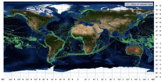
Figure 1. Ships’ distribution with type unknown in message1.

Existing ship classification methods, based on AIS data, generally consider static and dynamic information.

For static information, Damastuti et al. [9] use KNN (K-NearestNeighbor) to classify ships based on tonnage, length, and width in Indonesian waters and achieved an accuracy of up to 0.83 on six categories. Zhong et al. [10] use Random Forest for static information and achieve an accuracy of 0.865 on a three-classification task.

For dynamic information, Hong et al. [11] study the ships near the Ieodo Marine Research Station, and infer ship types by comparing the flag state of ships and the distribution of their corresponding trajectories with those of type-unknown ships. David et al. [12] use decision trees to identify fishing boats and achieve an accuracy of 0.8 and an F1 score of 0.7. Moreover, through conducting comparative experiments, they attempt to extract motion features as possible data. Sheng et al. [13] extract the COG (course over ground), ROT (rate of turn), and global features of vessels in the sea near Shantou, China, and use logistic regression to distinguish fishing and cargo vessels, achieving an accuracy of 0.923. Liang et al. [14] propose a multi-view feature fusion network that combines the CAE (convolutional auto-encoder) and the Bi-GRU (bidirectional gated recurrent unit) network to classify ships. They realize an accuracy of 95.51% and 94.24% in Luotou Channel and Qiongzhou Strait, respectively. Ginoulhac et al. [15] extract the statistical features from each temporal variable of AIS data, and the features are then input into a Gradient Boosting classifier; their method has an accuracy of 0.86. Xiang et al. [16] use p-GRUs (Partition-wise Gated Recurrent Units) to achieve the recognition of trawlers with an accuracy of 0.89. Another similar approach is presented in [17], which uses RNN (recurrent neural network) to classify five types of ships, with an accuracy of 0.783. In addition, some methods combine dynamic and static features. Kraus et al. [18] extract geographical distribution features, motion features, time of start/stop, and the static shape features of vessels from AIS data from German Bight and achieve an accuracy of 0.9751 on a five-classification task—however, the method has a data leakage problem. Kim et al. [19] integrate the vessel’s course change, speed, and environmental information (i.e., tide, light, and water temperature) to identify six types of fishing vessel activities in the waters around Jeju Island, achieving an accuracy of 0.963.

However, there still exists some disadvantages in the methods mentioned above, and they are summarized as follows.

• In some studies, only dynamic or static features are used for ship classification. As such, the utilization of multiple characteristics of ships is lacking, and the dynamic features are mainly set manually and empirically.
• Most of the existing studies use shore-based data which is usually distributed in a small area, for which the ship trajectories and motion features are restricted. For example, in inland rivers or ports, the ships’ position, speed, and direction are subject to limitations associated with the navigation channels, leading to an insufficient generalization ability of the classifier. Moreover, there is a lack of methods applicable to worldwide ship classification.
• The characteristics of space-based AIS data are different from those of shore-based data. Due to the limited number of satellites and the AIS signal conflict, global real-time coverage of AIS cannot currently be achieved. The continuity of space-based AIS data is weak, and there are few long-term ship trajectories with high continuity. The existing ship classification method may not be suitable for space-based AIS data.
• The classification number of ships in some researches is few, the differences between ships of different types are obvious, and the binary classification methods have limited application value.
• When splitting the sub-trajectories set, some researchers do not specifically distinguish the sources of sub-trajectories, which causes data from the same ship to appear in the training sets, validation sets, and testing sets. This data leakage problem will lead to the performance of the classifiers being overestimated.

To solve the problems outlined above, this paper proposes a multi-feature ensemble learning classification method (MFELCM) that integrates ships’ static and dynamic information. The method applies to the global range of satellite-based AIS data. The detailed process of MFELCM is shown in Figure 2, which consists of three steps. In the first step, the original data are preprocessed, and the cleaned static and dynamic data are then converted into static feature samples, dynamic feature distribution samples, time-series samples, and time-series feature samples. In the second step, four base classifiers, namely Random Forest [20], 1D-CNN (one-dimensional convolutional neural network) [21], Bi-GRU, and XGBoost (extreme gradient boosting) [22], are trained by the samples above. In the third step, another Random Forest is applied in order to integrate the base classifiers as MFELCM. The main contributions of this paper are as follows.

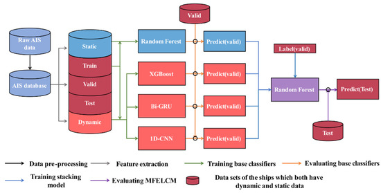
Figure 2. The overall process of MFELCM.

• A multiple-perspectives method of ship feature description is proposed in order to extract the dynamic and static features of ships from space-based AIS data.
• We propose the method to segment trajectories and split the data set by MMSI (Maritime Mobile Service Identity). The latter avoids the data leakage problem during the classifier training process.
• The proposed MFELCM, fusing the static and dynamic information, is suitable for the global wide space-based AIS data, which can update the type prediction with the continuous input of AIS data and achieve near real-time online classification. MFELCM can be applied in detecting the abnormal behaviors of ships and, thus, can enhance the capability of maritime supervision.
• The model parameters of MFELCM are determined by experiments, and it is verified that MFELCM outperforms the base classifiers. Moreover, when there are insufficient samples for a certain base classifier (e.g., dynamic feature distribution samples), the degraded MFELCM, integrated with the remaining base classifiers, can also achieve acceptable classification accuracy, which extends the application scope of MFELLCM.

The rest of this paper is organized as follows. In Section 2, the data from the ocean satellite HY-2B is taken as an example to present a basic introduction of space-based AIS data, including data pre-processing, data volume, and ship type distribution. Section 3 illustrates the detailed implementation of MFELCM, including static and dynamic features extraction, samples construction for different base classifiers, data set splitting, and the implementation of base classifiers. In Section 4, MFELCM is applied to the real AIS data, and the performance of the model is evaluated. In addition, we discuss the effectiveness of degraded MFELCM without a certain base classifier. Section 5 concludes the full paper and presents an expectation for future work.

2. AIS Data Pre-Processing

2.1. Data Preprocessing

Some fields in AIS messages are key information for classification. Considering that the dynamic features (from message1) should fully reflect the kinematic information of the ship at a specific moment, and the static features (from message5) should reflect the ship’s dimensions, draft, and type, we filter the key fields, as listed in Table 1, from the AIS message for ship classification. MMSI is the unique identification of a ship. The Time field in message1 is the time flag that is automatically injected by the space-based AIS receiver every minute [23], and it is accurate to a minute. Time Stamp is the UTC second when the AIS message is broadcasted. The exact time when the AIS message is sent can be obtained by combining the Time and Time Stamp. A, B, C, and D reflect the overall dimensions of the ship, which, respectively, represent the distances from the reference point O to the bow, stern, port side, and starboard of the ship, as shown in Figure 3. The ship length and width are calculated by Equation (1).

$$\left\{\begin{array}{c}length=A+B\\ width=C+D\end{array}\right.$$

(1)

Table 1. Fields selected from dynamic and static data.

Data	Fields Used
Dynamic (message1)	MMIS, Time, TimeStamp, Longitude, Latitude, SOG (Speed over ground), COG (Course over ground), ROT (Rate of turn)
Static (message5)	MMSI, A, B, C, D, Draught, Type

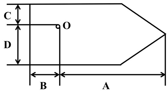
Figure 3. The overall dimension of a ship.

Raw AIS data may contain bad data, duplicate data, and missing data. In addition, the data format may be not convenient to analyze [24,25]. We perform the following data preprocessing operations on the fields in Table 1.

• If the field does not conform to the standards in [4], the message to which the field belongs is defined as an error message and should be removed.
• If all fields of several messages are the same, remove all but one message. For dynamic messages, if the duplicate fields are only MMSI, Time, and Time Stamp, all messages should be removed because we cannot determine the authenticity of these messages.
• In creating the Type field for message1, the values of Type are obtained from message5 by matching MMSI in mesage1 and message5.
• Replace the value seconds in the Time field of message1 with TimeStamp to obtain the exact moment the messages were sent.
• If there exists empty fields in a message, the message is defined as missing data. For dynamic messages, remove the missing data. For static messages, fill the empty fields with 0.

Equation (2) defines the preprocessed static and dynamic data. For a ship whose MMSI is $i_m$, $d_j^{i_m}$ is the jth dynamic data of this ship in time order, and $s^{i_m}$ is the static data of this ship. Moreover, Equation (3) defines the trajectory of this ship as a time series $T^{i_m}$.

$$\left\{\begin{array}{c}{d}_j^{i_m}={[tim{e}_j^{i_m},ln{g}_j^{i_m},la{t}_j^{i_m},SO{G}_j^{i_m},CO{G}_j^{i_m},RO{T}_j^{i_m},typ{e}^{i_m}]}^T\\ s^{i_m}={[A^{i_m},B^{i_m},C^{i_m},D^{i_m},draugh{t}^{i_m},typ{e}^{i_m}]}^T\end{array}\right.$$

(2)

$$T^{i_m}=[d_0^{i_m},d_1^{i_m},\cdots ,d_k^{i_m}]\cdots \cdots k>=1$$

(3)

2.2. Data Volume and Ship Distribution

The dynamic data used in this paper are extracted from message1 (noted as DYM1) received by the ocean satellite HY-2B from 1 November 2019 to 21 April 2020, and the ship distribution is shown in Figure 4. The static data are extracted from message5 (noted as STM5) received by ocean satellite HY-1C/D and HY-2B/C. The detailed information of DYM1 and STM5 is shown in Table 2.

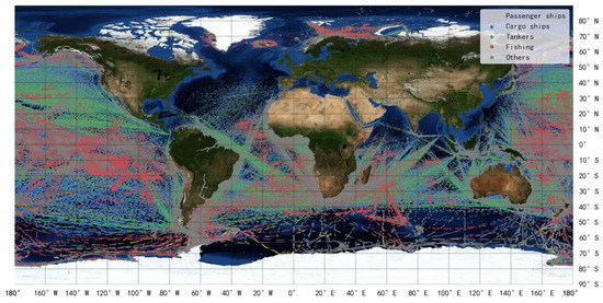
Figure 4. Message1 received by HY-2B.

Table 2. Information of message1 and message5.

Satellite	Data	Period	Number of Messages
HY-2B	Message1	1 November 2019~21 April 2020	10,875,328
HY-2B	Message5	1 November 2018~18 June 2021	113,472
HY-2C	Message5	24 September 2020~18 June 2021
HY-1C	Message5	1 November 2018~18 June 2021
HY-1D	Message5	13 June 2020~18 June 2021

In the literature [4], the value in the Type field of passenger ships, cargo ships, tankers, fishing boats, and tugs are 60 to 69, 70 to 79, 80 to 89, 30, and 52, respectively. The ships with code 0, 90, and a code larger than 99 have no specific type definition, and these ships are not considered in ship type statistics of space-based AIS data. Figure 5a,c show the number and cumulative percentage of the top 20 types of vessels in DYM1, counted by message quantity and ship (MMSI) quantity, which account for 96.62% and 95.37% of message1. In Figure 5b,d, four major categories of ships (i.e., passenger ships, tankers, fishing boats, and cargo ships) are used for type statistics, which account for 90.65% and 88.98% of message1 by message quantity and ship quantity. In this paper, these four kinds of ships are selected as the research object, and their global distribution is shown in Figure 4.

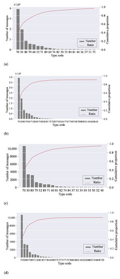
Figure 5. (a) Number and cumulative proportion of the top 20 ships (counted by message quantity); (b) Number and cumulative proportion of four types of ships (counted by message quantity); (c) Number and cumulative proportion of the top 20 ships (counted by MMSI quantity); (d) Number and cumulative proportion of four types of ships (counted by MMSI quantity).

3. Methodology

MFELCM integrates dynamic and static features of AIS data for ship classification. To realize MFELCM, the static feature dataset $SF$ and the dynamic feature datasets, i.e., $DFD$ (dynamic feature distribution dataset), $TS$ (time-series dataset), and $TSF$ (time-series feature dataset) are firstly constructed. The four base classifiers (i.e., Random Forest, 1D-CNN, Bi-GRU, and XGBoost) are then trained by $SF$, $DFD$, $TS$, and $TSF$, respectively. Finally, the MFELCM model is obtained by integrating the output of base classifiers using another Random Forest.

3.1. Static Feature Samples Construction

MFELCM integrates dynamic and static features of AIS data for ship classification. To realize MFELCM, the static feature dataset $SF$ and the dynamic feature datasets, i.e., $DFD$ (dynamic feature distribution dataset), $TS$ (time-series dataset), and $TSF$ (time-series feature dataset) are as follows.

For the static data $s^{i_m}$, five features, i.e., ship length, ship width, aspect ratio (ldivw), area, and ship girth, are added into $s^{i_m}$ according to Equations (1) and (4). The static data $s^{i_m}$ is redefined as Equation (5). In addition, the missing features in $s^i$ are filled with 0.

$$\left\{\begin{array}{c}ldivw=length/width\\ area=length\ast width\\ grith=length+width\end{array}\right.$$

(4)

$$s^{i_m}={[A^{i_m},B^{i_m},C^{i_m},D^{i_m},draugh{t}^{i_m},lengt{h}^{i_m},widt{h}^{i_m},ldiv{w}^{i_m},grit{h}^{i_m},typ{e}^{i_m}]}^T$$

(5)

As ship static information can be entered artificially, we should remove the unreasonable data before training classifiers. The distribution of static data is variable between the different types of ships, which makes it difficult to identify unreasonable data by a uniform standard for all categories. To filter the outliers, we first calculate the upper quartile ($Q_u$), the lower quartile ($Q_l$), and the interquartile ($IQR$) of a certain type of ship (e.g., passenger ships). If a feature in $s^{i_m}$ (e.g., $s^{i_m}$ belongs to a passenger ship) is outside $\left[Q_l-3IQR, Q_u+3IQR\right]$, then $s^{i_m}$ is recognized as an outlier and should be removed. We use this approach because it has no mandatory requirements on data distribution and is robust to outlier identification. A violin plot is the combination of box plot and KDE (kernel density estimation), and it can show the distribution of the variables. To illustrate the changes in the static features before and after removing outliers, we use a violin plot to visualize the static data, as shown in Figure 6. It should be noted that the data in Figure 6 is the static data after being standardized in accordance with the whole data set. Figure 6a,b are the distribution of original static data and the data having removed outliers of passenger ships, respectively. Figure 6c,d are the distribution of original static data and the data having removed outliers of four types of ships. Take Figure 6a as an example: the green part inside the red rectangle reflects part of the probability density function (PDF) of feature A, which takes the maximum value near the value where standardized A takes −2. The black part inside the blue rectangle represents the potential outliers judged by feature ldivw; the more the data is biased to both ends of the feature (i.e., ldivd) value, the more likely it is to be an outlier. By comparing Figure 6a–d, some obvious outliers are removed effectively.

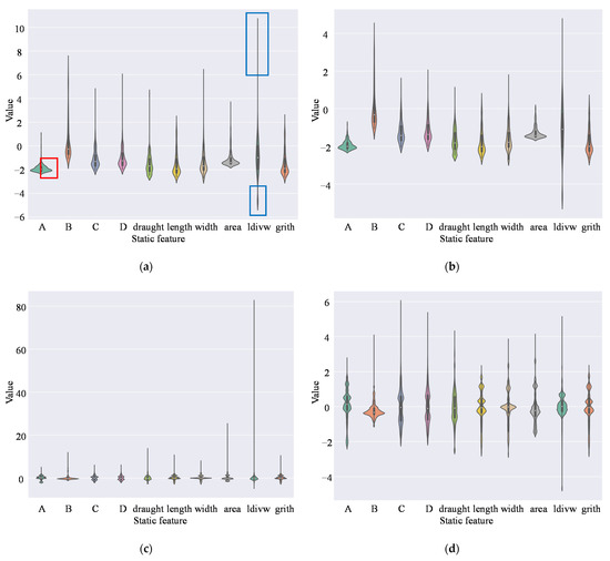
Figure 6. Distribution of original static data and the data after removing outliers. (a) Violin plot of passenger ships’ static features; (b) Violin plot of passenger ships’ static features (after removing outliers); (c) Violin plot of four types of ships’ static features; (d) Violin plot of four types of ships’ static feature (after removing outliers).

So far, we have obtained the static feature sample $s^{i_m}$. Let the set of all static feature samples be the static dataset SF, which is defined as Equation (6)

$$SF=\{s^{i_1},s^{i_2},\dots ,s^{i_m}\}$$

(6)

3.2. Dynamic Feature Samples Construction

For $d_{j+1}^{i_m}$ in $T^{i_m}$, add the features in Equation (7) into $d_{j+1}^{i_m}$, then $d_j^{i_m}$ is redefined as Equation (8). For $d_0^i$ in $T^i$, the supplementary features of $d_0^{i_m}$ defined by Equation (7) take the same value as those in $d_0^{i_m}$ except that $\delta t_0^{i_m}$, $\delta ln{g}_0^{i_m}$, $\delta la{t}_0^{i_m}$, $\delta CO{G}_0^{i_m}$, and $\delta SO{G}_0^{i_m}$ take the value zero.

$$\left\{\begin{array}{c}\delta t_{j+1}^{i_m}={\mathit{time}}_{j+1}^{i_m}-{\mathit{time}}_j^{i_m}\\ \delta {\mathit{lng}}_{j+1}^{i_m}={\mathit{lng}}_{j+1}^{i_m}-{\mathit{lng}}_j^{i_m}\\ \delta {\mathit{lat}}_{j+1}^{i_m}={\mathit{lat}}_{j+1}^{i_m}-{\mathit{lat}}_j^{i_m}\\ \delta {\mathit{COG}}_{j+1}^{i_m}={\mathit{COG}}_{j+1}^{i_m}-{\mathit{COG}}_j^{i_m}\\ {\mathit{ROT}}_{j+1}^{i_m{}^{\prime }}=\delta {\mathit{COG}}_{j+1}^{i_m}/\delta t_{j+1}^{i_m}\\ \delta {\mathit{SOG}}_{j+1}^{i_m}={\mathit{SOG}}_{j+1}^{i_m}-{\mathit{SOG}}_j^{i_m}\\ {\mathit{accelerate}}_{j+1}^{i_m{}^{\prime }}=\delta {\mathit{SOG}}_{j+1}^{i_m}/\delta t_{j+1}^{i_m}\\ {\mathit{speedlng}}_{j+1}^{i_m{}^{\prime }}=\delta {\mathit{lng}}_{j+1}^{i_m}/\delta t_{j+1}^{i_m}\\ {\mathit{speedlat}}_{j+1}^{i_m{}^{\prime }}=\delta {\mathit{lat}}_{j+1}^{i_m}/\delta t_{j+1}^{i_m}\\ {\mathit{speed}}_{j+1}^{i_m{}^{\prime }}={({{\mathit{speedlng}}_{j+1}^{i_m{}^{\prime }}}^2+{{\mathit{speedlat}}_{j+1}^{i_m{}^{\prime }}}^2)}^{-2}\end{array}\right.$$

(7)

$$\begin{array}{l}{d}_j^{i_m}=[tim{e}_j^{i_m},ln{g}_j^{i_m},la{t}_j^{i_m},SO{G}_j^{i_m},CO{G}_j^{i_m},RO{T}_j^{i_m},\delta t_j^{i_m},\delta ln{g}_j^{i_m},\delta la{t}_j^{i_m},\delta CO{G}_j^{i_m},RO{T}_j^{i_m{}^{\prime }},\\ \delta SO{G}_j^{i_m},accelerat{e}_j^{i_m{}^{\prime }},speedln{g}_j^{i_m{}^{\prime }},speedla{t}_j^{i_m{}^{\prime }},spee{d}_j^{i_m{}^{\prime }}{]}^T\end{array}$$

(8)

We add the features above into $d_{j+1}^i$ for the following reasons. The time interval $\delta t$ is associated with ships’ motion state [4] in Table A1. Sang et al. [26] and Kim et al. [19] pointed out that AIS equipment installed on different types of ships is of various cost and performance (e.g., fishing boats tend to install AIS equipment with low cost and accuracy), which may lead to the deviation of COG, SOG, ROT and other kinematic information. Considering the situation mentioned above, we calculate $RO{T}^{\prime }$, $accelerat{e}^{\prime }$, $speedln{g}^{\prime }$, $speedla{t}^{\prime }$, and $spee{d}^{\prime }$. Although the supplementary dynamic features may be redundant for ship motion state description, they can improve the anti-noise capability of the classifier.

As shown in Figure 7, we describe the trajectory $T^{i_m}$ from three aspects, which are $DF{D}^{i_m}$, $T{S}^{i_m}$, and $TS{F}^{i_m}$. $DF{D}^{i_m}$ is the distribution of the dynamic feature of $T^{i_m}$, which can reflect the overall motion characteristics of $T^{i_m}$. $T{S}^{i_m}$ is the set of sub-trajectories (e.g., $T{S}_n^{i_m}$) obtained from $T^{i_m}$, which reflects the short-term time series characteristics of $T^{i_m}$. ${[x_1,x_2,\dots ,x_k]}_n^{i_m}{}^T$ in $TS{F}^{i_m}$ is a feature vector extracted from $T{S}_n^{i_m}$, which reflects the short-term characteristics of $T^{i_m}$. Each element in ${[x_1,x_2,\dots ,x_k]}_n^{i_m}{}^T$ is a different feature calculated from $T{S}_n^{i_m}$, e.g., $x_1$ can be the average longitude of $T{S}_n^{i_m}$. $T{S}^{i_m}$ and $TS{F}^{i_m}$ are defined as Equations (9) and (10).

$$\left\{\begin{array}{c}T{S}^{i_m}=\{T{S}_1^{i_m},T{S}_2^{i_m},\dots ,T{S}_n^{i_m}\}\\ T{S}_n^{i_m}=[d_j^{i_m},d_{j+1}^{i_m},\dots ,d_{j+k}^{i_m}]\end{array}\right.$$

(9)

$$\left\{\begin{array}{c}TS{F}^{i_m}=\{TS{F}_1^{i_m},TS{F}_2^{i_m},\dots ,TS{F}_n^{i_m}\}\\ TS{F}_n^{i_m}={[x_1,x_2,\dots ,x_k]}_n^{i_m}{}^T\end{array}\right.$$

(10)

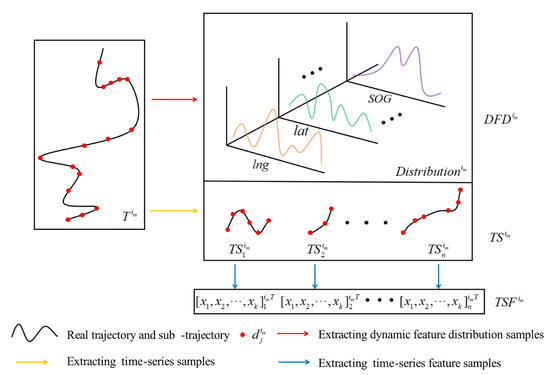
Figure 7. Process of dynamic features extraction.

3.2.1. Dynamic Feature Distribution Samples Dataset ($DFD$)

Let $DF{D}^{i_m}$ be the dynamic feature distribution of a ship whose MMSI is $i_m$, then $DFD$ is the set of $DF{D}^{i_m}$, which is defined by Equation (11).

$$DFD=\{DF{D}^{i_1},DF{D}^{i_2},\dots ,DF{D}^{i_m}\}$$

(11)

Limited by the number of satellites, signal conflicts, or AIS receiver performance [27,28], the dynamic data $d_j^{i_m}$ received by satellite is insufficient to describe $T^{i_m}$ completely. But in a longer period, for a trajectory $T^{i_m}$, the feature distribution function of $d_j^{i_m}$ can describe the overall motion of the ship (e.g., the distribution of latitude and longitude in Figure 7 describes the area of the ship’s activity). In addition, this description can reduce the impact of outliers. For the massive amount of space-based AIS data, it is impractical to calculate the feature distribution function for each $T^{i_m}$, so we use the frequency histogram to approximate the distribution function, as shown in Figure 8. For feature f of trajectory $T^{i_m}$, the range of f on the dataset is sliced uniformly into n intervals, on which the frequency distribution of f (i.e., $f_d$) is calculated. The matrix $DF{D}^{i_m}$ in Figure 8 is the combination of each feature’s frequency distribution. The Time field in $DF{D}^{i_m}$ is the number of minutes from the Time field in $d_j^{i_m}$ to the zero point of the day. $DF{D}^{i_m}$ takes 13 features into consideration, excluding the fields of $speedln{g}^{\prime }$,$speedla{t}^{\prime }$ and $spee{d}^{\prime }$.

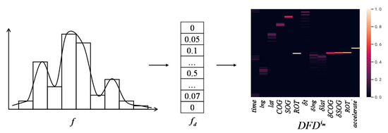
Figure 8. Process of extracting dynamic features distribution.

3.2.2. Time-Series Samples Dataset ($TS$)

$TS$ is defined as Equation (12), where $T{S}^{i_m}$ denotes the set of all sub-trajectories of $T^{i_m}$, as shown in Figure 7. Space-based AIS data has weak data continuity, and there are data points between which the time interval is large in $T^{i_m}$, which cannot reflect the ship movement correctly. As such, we break $T^{i_m}$ into a series of sub-trajectories $T{S}_n^{i_m}$. For $T^{i_m}$, the steps for constructing $T{S}^{i_m}$ are as follows.

$$TS=\{T{S}^{i_1},T{S}^{i_2},\dots ,T{S}^{i_m}\}$$

(12)

• Calculate the upper quartile $Q_u^{\delta t}$, the lower quartile $Q_l^{\delta t}$, and the quartile distance $IQ{R}^{\delta t}$ of the field $\delta t$ on the whole dynamic dataset.
• Traverse the points on $T^{i_m}$ in time order. For $d_j^{i_m}$, if $\delta t_j^{i_m}$ is outside [$Q_l^{\delta t}-3IQ{R}^{\delta t}, Q_u^{\delta t}+3IQ{R}^{\delta t}$], break $T^{i_m}$ at $d_{j-1}^{i_m}$, then set $\delta t_j^{i_m}$, $\delta ln{g}_j^{i_m}$, $\delta la{t}_j^{i_m}$, $\delta CO{G}_j^{i_m}$, and $\delta SO{G}_j^{i_m}$ to zero. The sequence from the last interrupted point to $d_{j-1}^{i_m}$ constructs the sub-trajectory $S{T}_n^{i_m}$. All sub-trajectories of $T^{i_m}$ construct $T{S}^{i_m}$.
• Apply the second step on all trajectories, and then we obtain $TS$.

3.2.3. Time-Series Feature Samples Dataset ($TSF$)

Denote $TS{F}^{i_m}$ as all feature vectors of sub-trajectories extracted from $T^{i_m}$, and then the time-series feature samples dataset $TSF$ is defined by Equation (13), as shown in Figure 7. Since it demands professional knowledge to point out the relationship between motion characteristics and the type of ships, we use a python toolkit named tsfresh (Time Series Feature extraction based on scalable hypothesis tests) [29] to generate ${[x_1,x_2,\dots ,x_k]}_n^{i_m}{}^T$ from $T{S}_n^{i_m}$ automatically.

$$\left\{\begin{array}{c}TSF=\{TS{F}^{i_1},TS{F}^{i_2},\dots ,TS{F}^{i_m}\}\\ TS{F}^{i_m}=\left\{TS{F}_1^{i_m},TS{F}_2^{i_m},\dots ,TS{F}_n^{i_m}\right\}\\ TS{F}_n^{i_m}={[x_1,x_2,\dots ,x_k]}_n^{i_m}{}^T\end{array}\right.$$

(13)

3.3. Dataset Segmentation

After obtaining the static dataset $SF$ and the dynamic datasets (i.e., $DFD$, $TS$, and $TSF$), the four datasets are split into training, validation, and testing sets. In the dynamic dataset, there is a correlation between the samples generated from the dynamic data of the same ship (e.g., ${[x_1,x_2,\dots ,x_k]}_1^{i_m}{}^T$ may be similar to ${[x_1,x_2,\dots ,x_k]}_n^{i_m}{}^T$). If we randomly split the dynamic datasets, samples from the same ship can simultaneously appear in training, validation, and testing sets, which will cause data leakage and the overestimation of the classifiers’ performance. In this paper, the datasets are split by the MMSI. Taking $TSF$ as an example, we divide $TSF$ at the level of $TS{F}^{i_m}$ rather than ${[x_1,x_2,\dots ,x_k]}_n^{i_m}{}^T$, i.e., once the $TS{F}^{i_m}$ is assigned to the training set, the feature vectors belonging to $T^{i_m}$ can only appear in the training set.

Ideally, the trajectory $T^{i_m}$ and the static feature sample $s^{i_m}$ are one-to-one correspondence. Due to the processing of removing outliers from static data in Section 3.1, there may be no $s^{i_m}$ corresponding to $T^{i_m}$. Furthermore, the dynamic data used in this paper is only a part of the whole dataset, which may result in no $T^{i_m}$ corresponding to $s^{i_m}$. To solve this problem, the MMSI in AIS data is divided into three parts, which are the MMSI that only appears in dynamic data (MMSI_D), the MMSI that only appears in static data (MMSI_S), and the MMSI which exists in both dynamic data and static data (MMSI_C), as shown in Figure 9. The MMSI_C is then divided into the MMSI training set (MMSI_TR), MMSI validation set (MMSI_V), and MMSI testing set (MMSI_T) by the stratified sampling of different types of ships. The static data, which is the MMSI in MMSI_S and MMSI_TR, forms the training set of static feature samples. The dynamic data, which is the MMSI in MMSI_D and MMSI_TR, forms the training set of dynamic feature samples. The static data, which is the MMSI in MMSI_V and MMSI_T, forms the validation set and the testing set of static feature samples, respectively. The dynamic data, which is the MMSI in MMSI_V and MMSI_T, forms the validation set and the testing set of dynamic feature samples, respectively.

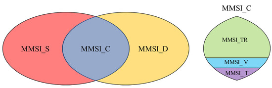
Figure 9. Split the datasets by MMSI.

For a trajectory $T^{i_m}$, if $i_m$ in MMSI_C, we can generate one $DF{D}^{i_m}$, n $T{S}_n^{i_m}$, and n $TS{F}_n^{i_m}$, which corresponds to one $s^{i_m}$. The number of static samples and dynamic samples with the same MMSI is different. To solve this problem, we copy $DF{D}^{i_m}$ and $s^{i_m}$ n times in $DFD$ and $SF$, respectively.

3.4. Implementation of MFELCM

3.4.1. Implementation of Random Forest

We use Random Forest to classify the static feature dataset $SF$. It is an integrated learning algorithm that is based on decision trees, which has the advantages of low bias, low variance, and high generalization ability. The method to create Random Forest is as follows.

• Select n samples from the training set randomly, which are used to create a decision tree. The decision tree is trained by the CART (Classification and Regression Tree) algorithm. In each node of a decision tree, m features of samples are randomly selected as an alternative set (AS) for node splitting. The feature k in AS and its threshold $t_k$ according to which the samples in this node are split into the left and the right nodes are then determined by minimizing the cost function, as shown in Equation (14). In Equation (14), $G_{left/right}$ and $m_{left/right}$ is the Gini Impurity and the number of samples of the left/right node, respectively. $G_{left/right}$ is calculated by Equation (15), in which $p_{i,j}$ is the proportion of class j samples in the ith node;

  $$J(k,t_k)=(m_{left}/m)\ast G_{left}+(m_{right}/m)\ast G_{right}$$

  (14)

  $$G_i=1-{\displaystyle \sum _{j=1}^q{p}_{i,j}^2}$$

  (15)
• When the decision tree reaches its maximum depth or the cost function cannot be reduced, stop node splitting and terminate the decision tree creation.
• Repeat the first step to create a large number of decision trees. We then obtain the Random Forest. When classifying the ship type, the decision trees vote on the class of the ship.

3.4.2. Implementation of 1D-CNN

Figure 10 shows the network structure of 1D-CNN. The details of 1D-CNN are shown in Table 3.

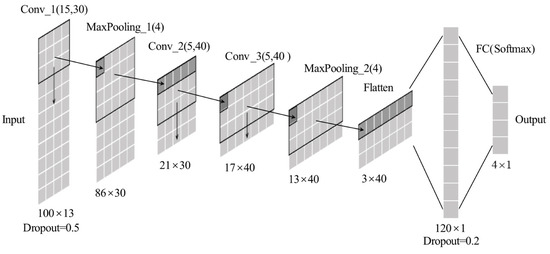
Figure 10. Structure of 1D-CNN.

Table 3. Details of 1D-CNN.

Layers	Shape	Input	Output	Activation Function	(Padding, Strides)
Conv_1 (Convolutional layer_1)	15 × 30	100 × 13	86 × 30	ELU (Exponential Linear Units)	(False,1)
MaxPooling_1	4 × 30	86 × 30	21 × 30	\	(False,1)
Conv_2	5 × 40	21 × 30	17 × 40	ELU	(False,1)
Conv_3	5 × 40	17 × 40	13 × 40	ELU	(False,1)
MaxPooling_2	4 × 40	13 × 40	3 × 40	\	(False,1)
Flatten layer	\	3 × 40	120 × 1	\	\
FC (Full connection layer)	\	120 × 1	4 × 1	Softmax	\

3.4.3. Implementation of Bi-GRU

To solve the short-term memory problem of the original RNN, Hochreiter, et al. [30] propose the long short-term memory (LSTM) unit. GRU [31] is the simplified version of LSTM. Figure 11 is the structure of a GRU unit, in which $g_t$ is the main layer and $r_t$ controls the reset gate, which resets $h_{t-1}$ based on $h_{t-1}$ (from the previous time step) and $x_t$ (from the current time step). The $h_{t-1}$ which has been reset is submitted to $g_t$. $z_t$ controls the forgetting gate as well as the output gate, which uses a ‘1-’ operation to ensure that the weight of the forgotten memory must be equal to the weight of the added memory at the current time step. The weights of $h_{t-1}$ to forget and that of $g_t$ to input into $h_{t-1}$ are determined by $h_{t-1}$ and $x_t$, Equation (16) shows the way to update the paraments of a GRU unit, where $W_{xz}, W_{xr}, W_{xg}$ and $W_{hz}, W_{hr}, W_{hg}$ are the connection weight matrixes of $x_t$ and $h_{t-1}$ to three fully connected layers. In addition, $b_z, b_r, b_g$ are the bias terms of three full connection layers, respectively.

$$\left\{\begin{array}{l}{z}_t=\sigma (W_{xz}^T{x}_t+W_{hz}^T{h}_{t-1}+b_z)\hfill \\ r_t=\sigma (W_{xr}^T{x}_t+W_{hr}^T{h}_{t-1}+b_r)\hfill \\ g_t=\tanh (W_{xg}^T{x}_t+W_{hg}^T(r_t\otimes h_{t-1})+b_g)\hfill \\ h_t=z_t\otimes h_{t-1}+(1-z_t)\otimes g_t\hfill \end{array}\right.$$

(16)

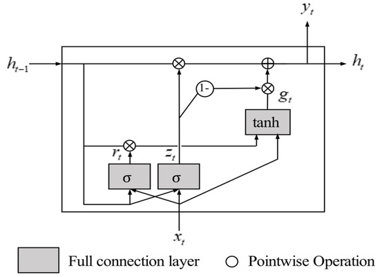
Figure 11. A GRU unit.

Figure 12 shows the structure of Bi-GRU. The time-series samples in a batch (e.g., $T{S}_1^{i_m}$, $T{S}_2^{i_m}$, and $T{S}_3^{i_m}$) are firstly filled with a value v to the same length. After going through the mask layer, the network will ignore the time step in which the data are filled with v. Bi-GRU is composed of a cyclic part and a full connection part. The cyclic part has four layers, and the hidden state of each layer in the cyclic part is 35 dimensions. The first layer in the cyclic part uses the bidirectional GRU, which enables the network to understand the behaviors of the previous time steps with the help of subsequent time steps. In this layer, for the GRU unit with input $d_j^{i_m}$, its output $y_j$ is obtained by concatenating $h_j$ (output in the forward direction) and $h_j^{\prime }$ (output in the reverse direction). The second layer and the third layer are the same unidirectional GRU network. The fourth layer outputs $y_{j+k}^{i_m}$ of the last time step and inputs it to two full connection layers. Finally, the network outputs a 4-dimensional vector, and the value (between 0 and 1) of each dimension in this vector represents the probability that $T{S}_n^{i_m}$ belongs to a certain class of ships.

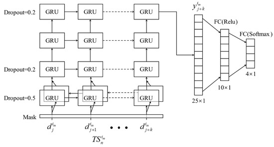
Figure 12. The framework of Bi-GRU.

The trajectory $T^{i_m}$ contains multiple time-series samples $T{S}_n^{i_m}$, and each $T{S}_n^{i_m}$ has its predicted type. As shown in Figure 13, to obtain the type of $T^{i_m}$, we must first calculate the mean value of the vectors whose $T{S}_n^{i_m}$ belonging to $T^{i_m}$, and we then take the category with the highest probability as the predicting type. Therefore, the classification performance evaluation of Bi-GRU includes two aspects. One is the performance of ship classification according to a single $T{S}_n^{i_m}$, and the other is the performance of ship classification by integrating all $T{S}_n^{i_m}$ from $T^{i_m}$. These two standards are also applicable to the based classifiers and MFELCM mentioned in this paper.

Figure 13. Prediction of Bi-GUR.

3.4.4. Implementation of XGBoost

XGBoost is an optimized implementation of Gradient Boosting Decision Tree (GBDT). The basic idea of GBDT is to build several Classification and Regression Trees (CARTs), and each CART fits the residual of the previous CART. The results of all CARTs are summed to obtain the prediction. The principle of XGBoost is explained in detail in the literature [21]. This article uses Python’s XGBoost toolkit to implement the XGBoost method.

3.4.5. Integration of the Base Classifiers

Since the base classifiers have extracted features from the samples, to avoid overfitting we use the Random Forest method to integrate the base classifiers, as it is relatively simple and has good interpretability. Figure 14 illustrates the process of base classifier integration. To prevent confusion, the Random Forest in base classifiers is denoted as Random Forest1, and the Random Forest in the integrated procedure is recorded as Random Forest2. In Figure 14, the output of the four base classifiers on the validation set and the real label of the validation set are input into the Random Forest2 to integrate the base classifiers. The four base classifiers and the Random Forest2 form the MFELCM model, and the performance of MFELCM is evaluated on the testing set.

Figure 14. The integration process of base classifiers.

4. Experimental Results and Analysis

The experiments of MFELCM are carried out on AIS data of four types of ships, i.e., passenger ships, tankers, fishing boats, and cargo ships, which are received by HY-1C/D and HY-2B/C. The experimental environment is Windows 10, Tensorflow 2.5.0, Keras 2.5.0, CPU is an AMD R7-5800H (3.2GHz), GPU is NVIDIA 3060 Laptop, and the memory is 32 G.

4.1. Overview of Experimental Data

For dynamic data, to reduce category imbalance and obtain effective ship dynamic features distribution, we select 300,000 pieces of messages from every four types of ships. Each ship should have more than 500 pieces of messages. Considering that the dynamic data should reflect ships’ motion features, the messages for which the SOG is lower than 2 knots are removed. The amount of dynamic data used in the experiments is shown in Table 4, and Figure 15 shows the data distribution.

Table 4. The number of original dynamic data.

Type	Number of Messages	Number of Ships
Passenger ships	233,131	189
Cargo ships	285,986	2161
Tankers	285,912	738
Fishing boats	213,442	674
Total	1,018,471	3762

Figure 15. Original dynamic data.

Too short sub-trajectories are insufficient to reflect the short-term motion state of the ships. When constructing the dynamic feature datasets (i.e., $DFD$, $TS$, and $TSF$), the sub-trajectories with less than 10 messages are ignored. The dynamic data used for experiments are shown in Table 5, and the data distribution is shown in Figure 16.

Table 5. The number of dynamic data used in experiments.

Type	Number of Messages	Number of Ships	Number of Sub-Trajectories
Passenger ships	162,351	151	7690
Cargo ships	167,457	1254	9035
Tankers	152,802	611	8555
Fishing boats	117,264	434	6411
Total	599,874	2450	31,691

Figure 16. Dynamic data used in experiments.

For static data, all static data of the four types of ships are extracted from the database. Table 6 shows the amount of data processed according to the method in Section 3.1. The number of static data messages is greater than the number of ships corresponding to the static data because the features in static messages may change sometimes (e.g., draught and position reference point), and there exists fraudulent use of MMSI.

Table 6. The number of static data.

Type	Number of Messages	Number of Ships
Passenger Ships	1285	1008
Cargo Ships	61,251	15,866
Tankers	21,094	6984
Fishing	5978	4565
Total	89,608	28,423

There are 2066 MMSI in MMSI_C (see Figure 9), and the dynamic and the static datasets are split according to the methods in Section 3.3. It should be noted that if one MMSI in MMSI_C corresponds to several $s^{i_m}$, those $s^{i_m}$ should be replaced by their average before the datasets are split.

4.2. Base Classifiers and MFELCM

Table 7 shows the evaluation of the base classifiers and MFELCM on the testing set, in which class 0 to class 3 represent passenger ships, tankers, fishing boats, and cargo ships, respectively.

$$\left\{\begin{array}{c}F1-score=(1/4){\displaystyle \sum _{i=1}^4{w}_i\times F1-scor{e}_i}\\ F1-scor{e}_i=2P_i{R}_i/(P_i+R_i)\\ P_i=T{P}_i/(T{P}_i+F{P}_i)\\ R_i=T{P}_i/(T{P}_i+F{N}_i)\end{array}\right.$$

(17)

Table 7. Performance evaluation of base classifiers and MFELCM.

Items		Evaluated on Samples					Evaluated on Ships
		Random Forest	1D-CNN	Bi-GRU	XGBoost	MFELCM	Random Forest	1D-CNN	Bi-GRU	XGBoost	MFELCM
Accuracy	class0	0.9931	0.9217	0.7191	0.8548	0.9985	0.8889	0.6667	0.6667	0.7778	0.8889
	class1	0.9320	0.7861	0.6052	0.5467	0.9344	0.9237	0.6271	0.6864	0.6102	0.9322
	class2	0.9340	0.8879	0.7690	0.8117	0.9332	0.9032	0.7903	0.7419	0.8065	0.9355
	class3	0.8244	0.6173	0.5972	0.6839	0.8797	0.8287	0.7315	0.6296	0.7546	0.8750
Total Accuracy		0.9205	0.7914	0.6566	0.7008	0.9362	0.8696	0.7077	0.6643	0.7222	0.9010
F1 score		0.9196	0.7873	0.6629	0.6991	0.9359	0.8719	0.7127	0.6681	0.7239	0.9019

F1 score is calculated by Equation (17). $T{P}_i$, $F{P}_i$ and $F{N}_i$ are the number of true positive, false positive, and false-negative samples of type i ships, respectively. $P_i$ and $R_i$ are the accuracy and the recall of the model in classifying class i samples, respectively. The F1 score of a model is the weighted average of F1 scores for each type of ship, and the weight $w_i$ is the proportion of class i samples in the total number of samples. In addition, to reduce the effect of sample imbalance, the loss of samples is weighted during the training process, and the weight of the class i samples is set as $w_i{}^{-1}$.

4.2.1. Random Forest1 Experimental Results

The optimal hyper-parameters of the Random Forest1 are determined by random search, as shown in Table 8. Figure 17 is the confusion matrixes of the classifier on the testing set. The model tends to confuse passenger ships with fishing boats, and confuse tankers with cargo ships.

Table 8. Hyper-parameters used in Random Forest.

Hyper-Parameters	Value
max_depth	10
max_leaf_nodes	58
min_samples_leaf	77
n_estimators	1500

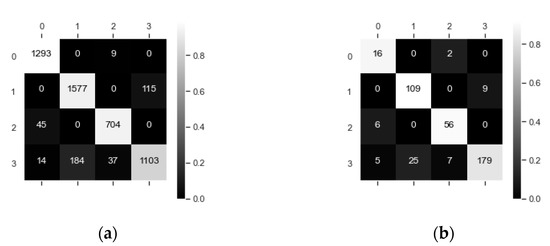
Figure 17. (a) Confusion matrix of samples (Random Forest1); (b) Confusion matrix of ships (Random Forest1).

To explain the confusion matrixes, we use t-SNE [32] to visualize the static features. t-SNE is a method of data visualization which can map data from high-dimensional space to low-dimensional space. If two samples are similar in high-dimensional space, the distance between their maps in low-dimensional space will be close. Figure 18 shows the visual results of static features. There are partial overlaps between the reduced dimensional distributions of passenger ships and fishing vessels, as well as that of tankers and cargo ships, which implies that the static information of the misclassified ships is similar.

Figure 18. Visualization of static features.

Figure 19 shows the importance of the static information features. It can be seen that the ship’s dimensional characteristics, such as A, length, and length-width ratio, can better describe the ships’ features than draught. In addition, although the features C and D contribute little to the classifier, these two parameters have been reflected in the length-width ratio, girth, area, and width, which proves that the static features constructed in this paper are effective in the ship classification task.

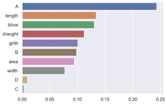
Figure 19. Static feature importance.

4.2.2. 1D-CNN Experimental Results

The number and the width of the convolution kernels in the first convolution layer (Conv_1) in 1D-CNN are optimized using grid search, as shown in Table 9. The model used an Adam optimizer with a learning rate of 1 × 10⁻³, a batch size of 2500, and the cross-entropy loss function. Figure 10 shows the structure of 1D-CNN. 1D-CNN performs best when the parament of Conv_1 is Conv (30,15).

Table 9. Parameters of the first convolution layer.

Parameters of Conv1 Conv (Number, Width)	F1 Score		Accuracy
	Evaluated on Samples	Evaluated on Ships	Evaluated on Samples	Evaluated on Ships
Conv (10,5)	0.5758	0.5373	0.6068	0.5169
Conv (10,10)	0.6248	0.5883	0.6530	0.5749
Conv (10,15)	0.6131	0.5533	0.6538	0.5483
Conv (10,20)	0.6385	0.5590	0.6796	0.5580
Conv (10,25)	0.6380	0.5809	0.6759	0.5797
Conv (20,5)	0.6244	0.6010	0.6463	0.5797
Conv (20,10)	0.7218	0.6276	0.7467	0.6232
Conv (20,15)	0.7274	0.6378	0.7451	0.6353
Conv (20,20)	0.7167	0.6844	0.7217	0.6739
Conv (20,25)	0.7660	0.6739	0.7748	0.6715
Conv (30,5)	0.6907	0.6719	0.6973	0.6546
Conv (30,10)	0.6845	0.6342	0.7036	0.6280
Conv(30,15)	0.7873	0.7128	0.7914	0.7077
Conv (30,20)	0.7388	0.7121	0.7398	0.7029
Conv (30,25)	0.7717	0.6754	0.7786	0.6715

Figure 20 plots the learning curve of 1D-CNN. Figure 21 shows the confusion matrixes of 1D-CNN on the testing set, where the classifier tends to confuse passenger ships with fishing boats, as well as tankers with cargo ships.

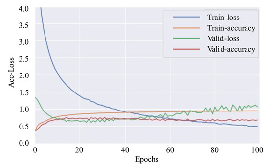
Figure 20. Learning curve (1D-CNN).

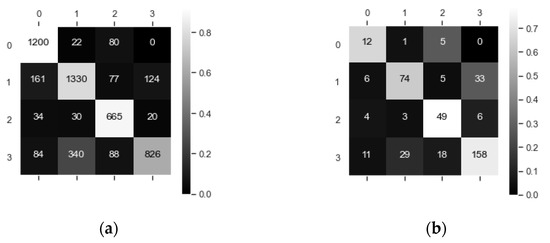
Figure 21. (a) Confusion matrix of samples (1D-CNN); (b) Confusion matrix of ships (1D-CNN).

Figure 22a visualizes 30 convolutional kernels of Conv_1, each of which is a 15 × 13 matrix. Figure 22b shows the matrix Q added to by the 30 convolution kernels in Conv_1. Figure 22c shows the result of taking the absolute value after summing the matrix Q according to the columns. Convolution realizes the dimension reduction and feature extraction from the original data. In the first convolution layer, the value of the convolution kernel in different columns reflects the response intensity of the network to different characteristics. By summing Q and taking the absolute value, the importance of features for 1D-CNN can be inferred.

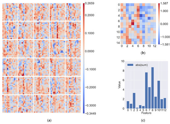
Figure 22. (a) Convolution kernel of the Conv_1; (b) Results of convolution kernel summation (matrix Q); (c) Sum Q by columns and take the absolute value.

In Figure 22c, the features from 0 to 12 correspond to the features of $DF{D}^{i_m}$ in Figure 8. As we can see from Figure 22c, the four most important features to 1D-CNN are $\delta lat$, $\delta t$, $\delta SOG$, and $\delta lon$. The combination of $\delta lat$ and $\delta lon$ can reflect the directional information of ship motion. According to Table A1, $\delta t$ is associated with ships motion state, and the combination of these four features (i.e., $\delta lat$, $\delta t$, $\delta SOG$, and $\delta lon$) can reflect the information of ship’s speed, acceleration, and steering rate. In Figure 4, it is obvious that there are some routes for cargo ships and tankers around the world, and the ship’s direction within the routes is usually fixed. However, the movements of fishing boats and passenger ships are more variable. Based on the above analysis, we speculate that the 1D-CNN network may learn the movement characteristics of different types of ships on the routes. In addition, the time feature contributes little to 1D-CNN, which is probably because most of the ships do not have such features, except for some offshore or inland river ships, which have regular activity periods in a day. The reason why the classifier confuses the samples (see Figure 21) may be that the features of interest to 1D-CNN have some similarities between oil tankers and cargo ships, and between passenger ships and fishing boats.

4.2.3. Bi-GRU Experimental Results

The number of cells in the hidden layer (NoC) of Bi-GRU is optimized using random search, as shown in Table 10. The model structure is shown in Figure 12. The model used an Adam optimizer with a learning rate of 1e-3, a batch size of 1500, and the cross-entropy loss function. In Figure 12, as we prefer to choose the model with better performance on ship classification, the NoC of Bi-GRU is set to 35. Figure 23 plots the learning curve of Bi-GRU. Figure 24 shows the confusion matrixes of Bi-GRU on the testing set. In Figure 24a, part of the sub-trajectories of passenger ships are misclassified into three other categories, and there is confusion between tankers and cargo ships, and some sub-trajectories of fishing boats are misclassified into cargo ships. In Figure 24b, the classifier confuses passenger ships with fishing boats, as well as tankers with cargo ships, and some fishing boats are mislabeled as cargo ships.

Table 10. Unit number in the hidden layer.

NoC	F1 Score		Accuracy
	Evaluated on Samples	Evaluated on Ships	Evaluated on Samples	Evaluated on Ships
15	0.6252	0.6158	0.6219	0.6159
20	0.6387	0.6328	0.6335	0.6329
25	0.6496	0.6435	0.6455	0.6425
30	0.6586	0.6370	0.6546	0.6353
35	0.6629	0.6681	0.6566	0.6643
40	0.6726	0.6539	0.6690	0.6521
45	0.6605	0.6381	0.6575	0.6327

Figure 23. Learning curve (Bi-GRU).

Figure 24. (a) Confusion matrix of sub-trajectories (Bi-GRU); (b) Confusion matrix of ships (Bi-GRU).

4.2.4. XGBoost Experimental Results

The maximum depth of trees in XGBoost is 20 and the learning rate is 0.03.

The python toolkit named tsfresh can automatically generate a large number of features from time series, but it requires a lot of computing resources. In addition, many features are useless for classification, and thus it is necessary to filter the features outputted by tsfresh, which is done as follows.

• Step 1. Extract features without filtering using tsfresh on a small dataset M and create the time-series dataset of M (denoted as $TS\left(M\right)$), and then use $TS\left(M\right)$ to train an XGBoost (denoted as XGBoost1).
• Step 2. Use XGBoost1 to output the top n important features on dataset M.
• Step 3. Use tsfresh to extract the n features obtained in Step 2 on the dynamic dataset (Table 5), and create the time-series dataset (denoted as $TS$), then use $TS$ to train another XGBoost (denoted as XGBoost2).
• Step 4. If n is not zero, return to Step 2 and decrease n with a certain interval.
• Step 5. When n can no longer decrease, choose the XGBoost2 with the best performance obtained in Step 3. The features used by this model are the most important feature that is generated by tsfresh.

We select 50,000 dynamic messages from the four types of ships, and each ship should have more than 500 pieces of messages. After removing those sub-trajectories which contain less than 10 pieces of messages, there are 106,169 pieces of dynamic messages left, which is the dataset M. Table 11 illustrates the amount of M, whose distribution is shown in Figure 25. The XGBoost1 is trained on $TS\left(M\right)$ with 3765 features extracted from M by tsfresh. Figure 26 shows the importance of the features outputted by XGBoost1. Table 12 shows the performance of XGBoost2 which trains on $TS$ with a different number of features. The XGBoost2 performs best when the top 40 important features are considered. The features’ names and weights are shown in Table A2, and the detailed definition of these features can be obtained from [33].

Table 11. The amount of data in dataset M.

Type	Number of Messages	Number of Ships	Number of Sub-Trajectories
Passenger Ships	28,513	135	1197
Cargo Ships	27,984	249	1494
Tankers	28,818	289	1493
Fishing boats	20,854	104	1084
Total	106,169	777	5268

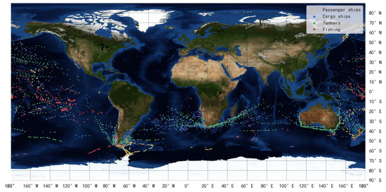
Figure 25. Ships distribution of dataset M.

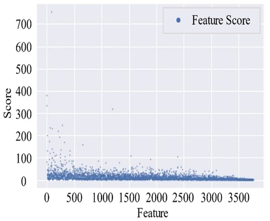
Figure 26. Features and their importance score on dataset M.

Table 12. XGBoost2 trained by different features.

Number of Features	F1 Score		Accuracy
	Evaluated on Samples	Evaluated on Ships	Evaluated on Samples	Evaluated on Ships
100	0.7083	0.7136	0.7103	0.7126
80	0.7086	0.7163	0.7107	0.7126
60	0.6986	0.7052	0.7010	0.7029
40	0.6991	0.7239	0.7008	0.7222
20	0.6872	0.6715	0.6906	0.6691

When using 40 features to complete the classification of ships, the learning curve of XGBoost2 and the confusion matrix on the testing set are as shown in Figure 27. In Figure 27b, some sub-trajectories of passenger ships are misclassified into the other three categories. The classifier tends to confuse tankers with cargo ships, and tankers are more likely to be mislabeled as cargo ships. In Figure 27c, the confusion of tankers and cargo ships remains significant. Figure 28 shows the importance score of these 40 features, whose names and values of importance score are shown in Table A2. The features are mostly related to the location, speed, heading, and steering rate information of the ships, and we infer that the XGBoost2 tends to learn ships’ spatial distribution.

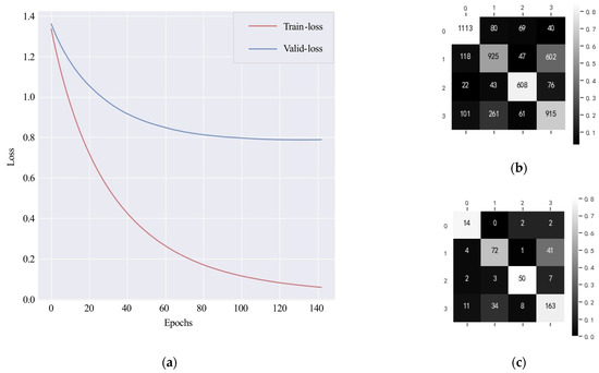
Figure 27. (a) Learning curve (XGBoost2); (b) Confusion matrix of samples (XGBoost); (c) Confusion matrix of ships (XGBoost2).

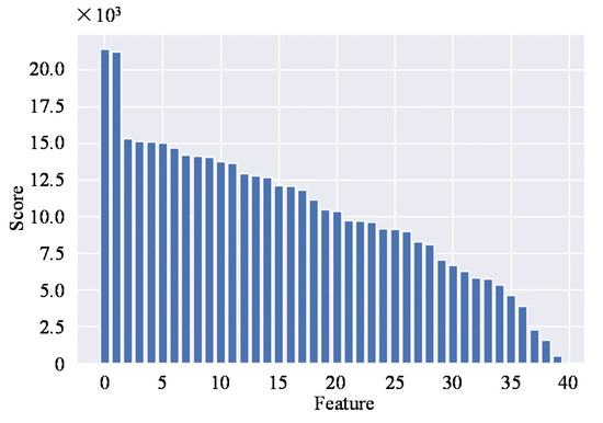
Figure 28. Top 40 most important features.

In addition, we carry out an experiment to illustrate the necessity of splitting the dataset by MMSI. The XGBoost trained on the time-series feature dataset $TSF$ ($TSF$ is split by $TS{F}_n^{i_m}$ instead of $TS{F}^{i_m}$) is denoted as XGBoost3. Under the same parameters with XGBoost2, the learning curve and the confusion matrixes of XGBoost3 are shown in Figure 29. The F1 score and total accuracy of XGBoost3 evaluated on $TS{F}^{i_m}$ are 0.8180 and 0.8186, respectively, and those evaluated on ships are 0.7996 and 0.7994. It seems that the XGBoost3 performs better than the XGBoost2, but this is because the samples ($TS{F}^{i_m}$) from the same ship ($TS{F}^{i_m}$) appear in the training set and the testing/validation set at the same time. This data leakage leads to the performance of XGBoost3 being overestimated.

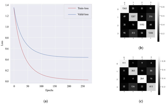
Figure 29. (a) Learning curve (XGBoost3); (b) Confusion matrix of samples (XGBoost3); (c) Confusion matrix of ships (XGBoost3).

4.2.5. MFELCM Experimental Results

The Random Forest (denoted as Random Forest2) is used to integrate four base classifiers, and MFELCM is the combination of four base classifiers and Random Forest2. The weight of class i of samples (i.e., samples in Figure 14) is the ratio of the total number of samples to the number of class i samples. The best paraments of Random Forest2 are shown in Table 13, and are obtained by random search. The weights of Random Forest2 to each base classifier are shown in Figure 30. Figure 31 shows the confusion matrixes of Random Forest2 on the validation set (which is also the confusion matrixes of MFELCM). Comparing the performance of MFELCM with the base classifiers in Table 5, MFELCM has higher total accuracy and F1 score than those of the base classifiers. Specifically, MFELCM reduces the confusion between passenger ships and fishing boats, as well as that between tankers and cargo ships. When evaluating the performance of MFELCM by samples, MFELCM improves the total accuracy by 1.57% and the F1 score by 1.63%, which is equivalent to a 24.61% reduction in misclassification over the best base classifiers (Random Forest1). When evaluating the performance of MFELCM by ships, MFELCM improves the total accuracy by 3.14% and F1 score by 3%, which is equivalent to a 24.08% reduction in misclassification over the best base classifiers (Random Forest1). Different classifiers focus on different ship features and they have different classification tendencies. By integrating multiple features, MFELCM reduces the bias effectively. Furthermore, the classification results of ships can be refreshed by updating the dynamic information regularly (e.g., using satellites to transmit and update data regularly), which enables near real-time online classification.

Table 13. Parameters of Random Forest2.

Parameters	Value
max_depth	57
max_leaf_nodes	40
min_samples_leaf	9
n_estimators	1500

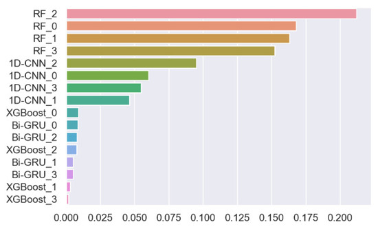
Figure 30. MFELCM feature importance.

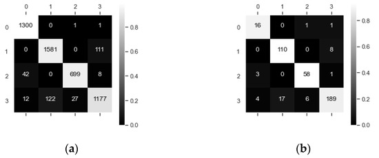
Figure 31. (a) Confusion matrix of samples (MFELCM); (b) Confusion matrix of ships (MFELCM).

4.3. The Degraded MFELCM

In practice, space-based AIS data may not provide the features required by the four base classifiers at the same time. The classification effect of degraded MFELCM with one base classifier absence is discussed below.

When the static features are missing, the degraded MFELCM (denoted as MFELCM1) integrates 1D-CNN, Bi-GRU, and XGBoost. The paraments of Random Forest2 in MFELCM1 are shown in Table 14. The weights of Random Forest2 to each base classifier are shown in Figure 32. Figure 33 shows the confusion matrixes of MFELCM1 on the testing set. Table 15 compares the performance of MFELCM1 with the base classifiers, and MFELCM1 is better than the base classifiers in terms of the total accuracy and F1 score. In addition, MFELCM1 can either refresh the classification results by updating the inputs or can switch to MFELCM when receiving static features.

Table 14. Parameters of Random Forest2 (in MFELCM1).

Parameters	Value
max_depth	45
max_leaf_nodes	11
min_samples_leaf	41
n_estimators	1000

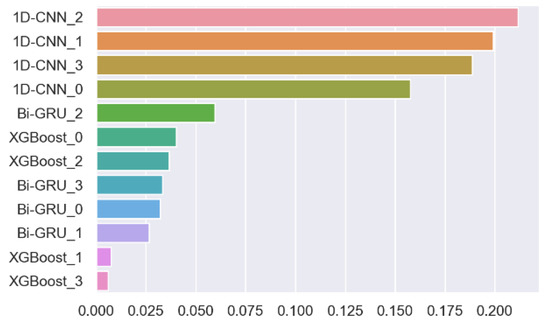
Figure 32. MFELCM1 feature importance.

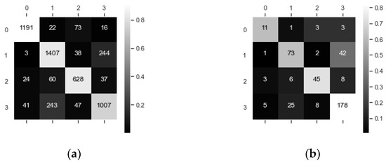
Figure 33. (a) Confusion matrix of samples (MFELCM1); (b) Confusion matrix of ships (MFELCM1).

Table 15. Performance evaluation of base classifiers and MFELCM1.

Items		Evaluated on Samples				Evaluated on Ships
		1D-CNN	Bi-GRU	XGBoost	MFELCM1	1D-CNN	Bi-GRU	XGBoost	MFELCM1
Accuracy	class 0	0.9217	0.7191	0.8548	0.9147	0.6667	0.6667	0.7778	0.6111
	class 1	0.7861	0.6052	0.5467	0.8316	0.6271	0.6864	0.6102	0.6186
	class 2	0.8879	0.7690	0.8117	0.8385	0.7903	0.7419	0.8065	0.7258
	class3	0.6173	0.5972	0.6839	0.7526	0.7315	0.6296	0.7546	0.8241
Total Accuracy		0.7914	0.6566	0.7008	0.8331	0.7077	0.6643	0.7222	0.7415
F1 score		0.7873	0.6629	0.6991	0.8334	0.7127	0.6681	0.7239	0.7396

In the case of missing dynamic feature distribution due to insufficient dynamic data, the degraded MFELCM (noted as MFELCM2) integrates Random Forest1, Bi-GRU, and XGBoost. The paraments of Random Forest2 in MFELCM2 are shown in Table 16. The weights of Random Forest2 to each base classifier are shown in Figure 34. Figure 35 shows the confusion matrixes of MFELCM2 on the testing set. Table 17 compares the performance of MFELCM2 with the base classifiers. MFELCM2 outperforms the base classifiers in terms of the total accuracy and F1 score. In addition, MFELCM2 can either refresh the classification prediction by updating the inputs or can switch to MFELCM after receiving a sufficient amount of dynamic data.

Table 16. Parameters of Random Forest2 (in MFELCM2).

Parameters	Value
max_depth	37
max_leaf_nodes	9
min_samples_leaf	61
n_estimators	2000

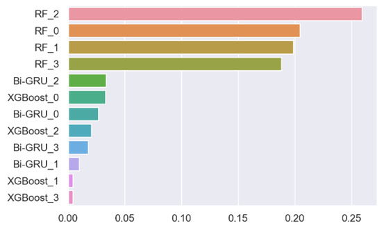
Figure 34. MFELCM2 feature importance.

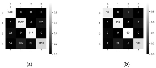
Figure 35. (a) Confusion matrix of samples (MFELCM2); (b) Confusion matrix of ships (MFELCM2).

Table 17. Performance evaluation of base classifiers and MFELCM2.

Items		Evaluated on Samples				Evaluated on Ships
		Random Forest	Bi-GRU	XGBoost	MFELCM2	Random Forest	Bi-GRU	XGBoost	MFELCM2
Accuracy	class 0	0.9931	0.7191	0.8548	0.9892	0.8889	0.6667	0.7778	0.8889
	class 1	0.9320	0.6052	0.5467	0.9261	0.9237	0.6864	0.6102	0.9237
	class 2	0.9340	0.7690	0.8117	0.9573	0.9032	0.7419	0.8065	0.9677
	class3	0.8244	0.5972	0.6839	0.8296	0.8287	0.6296	0.7546	0.8333
Total Accuracy		0.9205	0.9205	0.7008	0.9215	0.8696	0.8696	0.7222	0.8816
F1 score		0.9196	0.9196	0.6991	0.9207	0.8719	0.8719	0.7239	0.8822

5. Conclusions and Future Work

In this paper, we propose a ship classification method named MFELCM which is suitable for space-based AIS data worldwide. MFELCM integrates four base classifiers, i.e., Radom Forest, 1D-CNN, Bi-GRU, and XGBoost. The dynamic and static data are firstly preprocessed and four datasets are constructed (i.e., the static feature dataset $SF$, the dynamic feature distribution dataset $DFD$, the time-series dataset $TS$, and the time-series feature dataset $TSF$), after which the datasets are split by MMSI to avoid the data leakage problem. Finally, the base classifiers are integrated by another Random Forest. Experiments show that MFELCM performs better than the four base classifiers, and MFELCM can effectively integrate the static and dynamic information of ships. Moreover, in the case of one base classifier being missing, the degraded MFELCM—which integrates the remaining base classifiers—still outperforms the base classifiers. As MFELCM integrates multiple features, it can achieve near real-time online classification, which can be applied to ship behavior anomaly detection as well as enhancing the supervision of maritime activities.

The methods used to generate the dynamic features are an important factor for classification performance. In addition, the parameters of the classifiers are obtained by experiments in this paper. In the future, to further improve the performance of MFELCM, we plan to refine the methods of dynamic features generation as well as develop an automatic classifier parameter optimization method.

References

- Pallotta, G.; Vespe, M.; Bryan, K. Vessel Pattern Knowledge Discovery from AIS Data: A Framework for Anomaly Detection and Route Prediction. Entropy 2013, 15, 2218–2245. [Google Scholar] [CrossRef]
- Rong, H.; Teixeira, A.P.; Soares, C.G. Ship trajectory uncertainty prediction based on a Gaussian Process model. Ocean Eng. 2019, 182, 499–511. [Google Scholar] [CrossRef]
- Sheng, P.; Yin, J. Extracting Shipping Route Patterns by Trajectory Clustering Model Based on Automatic Identification System Data. Sustainability 2018, 10, 2327. [Google Scholar] [CrossRef]
- Technical Characteristics for an Automatic Identification System Using Time-Division Multiple Access in the VHF Maritime Mobile Band, Recommendation ITU-R M.1371-4. 2010, Volume 3–4, pp. 101–107. Available online: https://www.itu.int/dms_pubrec/itu-r/rec/m/R-REC-M.1371-5-201402-I!!PDF-E.pdf (accessed on 24 September 2021).
- Li, S.; Chen, L.; Chen, X.; Zhao, Y.; Bai, Y. Long-range AIS Message Analysis based on the TianTuo-3 Micro Satellite. Acta Astronaut. 2017, 136, 159–165. [Google Scholar] [CrossRef]
- Iphar, C.; Napoli, A.; Ray, C. Detection of false AIS messages for the improvement of maritime situational awareness. In Proceedings of the OCEANS 2015—MTS/IEEE, Washington, DC, USA, 19–22 October 2015; pp. 1–7. [Google Scholar] [CrossRef]
- Harati, A.; Wall, A.; Brooks, P.; Wang, J. Automatic Identification System (AIS): Data Reliability and Human Error Implications. J. Navig. 2007, 60, 373–389. [Google Scholar] [CrossRef]
- Longépé, N.; Hajduch, G.; Ardianto, R.; de Joux, R.; Nhunfat, B.; Marzuki, M.I.; Fablet, R.; Hermawan, I.; Germain, O.; Subki, B.A.; et al. Completing fishing monitoring with spaceborne Vessel Detection System (VDS) and Automatic Identification System (AIS) to assess illegal fishing in Indonesia. Mar. Pollut. Bull. 2018, 131, 33–39. [Google Scholar] [CrossRef]
- Damastuti, N.; Siti Aisjah, A. Classification of Ship-Based Automatic Identification Systems Using K-Nearest Neighbors. In Proceedings of the 2019 International Seminar on Application for Technology of Information and Communication (iSemantic), Semarang, Indonesia, 21–22 September 2019; pp. 331–335. [Google Scholar] [CrossRef]
- Zhong, H.; Song, X.; Yang, L. Vessel Classification from Space-based AIS Data Using Random Forest. In Proceedings of the 2019 5th International Conference on Big Data and Information Analytics (BigDIA), Kunming, China, 8–10 July 2019; pp. 9–12. [Google Scholar] [CrossRef]
- Hong, D.; Yang, C. Classification of Passing Vessels around the Ieodo Ocean Research Station Using Automatic Identification System (AIS): 21–30 November 2013. J. Korean Soc. Mar. Environ. Energy 2014, 17, 297–305. [Google Scholar] [CrossRef]
- Sánchez Pedroche, D.; Amigo, D.; García, J.; Molina, J.M. Architecture for Trajectory-Based Fishing Ship Classification with AIS Data. Sensors 2020, 20, 3782. [Google Scholar] [CrossRef]
- Sheng, K.; Liu, Z.; Zhou, D.; He, A.; Feng, C. Research on Ship Classification Based on Trajectory Features. J. Navig. 2018, 71, 100–116. [Google Scholar] [CrossRef]
- Liang, M.; Zhan, Y.; Liu, R.W. MVFFNet: Multi-view feature fusion network for imbalanced ship classification. Pattern Recognit. Lett. 2021, 151, 26–32. [Google Scholar] [CrossRef]
- Ginoulhac, R.; Barbaresco, F.; Schneider, J.; Pannier, J.; Savary, S. Target classification based on kinematic data from AIS/ADS-B, using statistical features extraction and boosting. In Proceedings of the 2019 20th International Radar Symposium (IRS), Ulm, Germany, 26–28 June 2019; pp. 1–10. [Google Scholar] [CrossRef]
- Jiang, X.; Liu, X.; Souza, E.N.; Hu, B.; Silve, D.L.; Matwin, S. Improving point-based AIS trajectory classification with partition-wise gated recurrent units. In Proceedings of the 2017 International Joint Conference on Neural Networks (IJCNN), Anchorage, AK, USA, 14–19 May 2017; pp. 4044–4051. [Google Scholar] [CrossRef]
- Bakkegaard, S.; Blixenkrone-Moller, J.; Larsen, J.J.; Jochumsen, L. Target classification using kinematic data and a recurrent neural network. In Proceedings of the 2018 19th International Radar Symposium (IRS), Bonn, Germany, 20–22 June 2018. [Google Scholar] [CrossRef]
- Kraus, P.; Mohrdieck, C.; Schwenker, F. Ship classification based on trajectory data with machine-learning methods. In Proceedings of the 2018 19th International Radar Symposium (IRS), Bonn, Germany, 20–22 June 2018. [Google Scholar] [CrossRef]
- Kim, K.I.; Lee, K.M. Convolutional Neural Network-Based Gear Type Identification from Automatic Identification System Trajectory Data. Appl. Sci. 2020, 10, 4010. [Google Scholar] [CrossRef]
- Andy, L.; Matthew, W. Classification and Regression by RandomForest. Forest 2001, 2, 18–22. [Google Scholar]
- Mitiche, I.; Nesbitt, A.; Conner, S.; Boreham, P.; Morison, G. 1D-CNN based real-time fault detection system for power asset diagnostics. IET Gener. Transm. Distrib. 2020, 14, 5766–5773. [Google Scholar] [CrossRef]
- Chen, T.; Guestrin, C. XGBoost: A Scalable Tree Boosting System. In Proceedings of the 22nd ACM SIGKDD International Conference on Knowledge Discovery and Data Mining, New York, NY, USA, 24–27 August 2016; pp. 785–794. [Google Scholar] [CrossRef]
- Li, S.; Chen, X.; Chen, L.; Zhao, Y.; Sheng, T.; Bai, Y. Data Reception Analysis of the AIS on board the TianTuo-3 Satellite. J. Navig. 2017, 70, 761–774. [Google Scholar] [CrossRef]
- Kotsiantis, S.B. Supervised Machine Learning: A Review of Classification Techniques. Informatica 2007, 31, 249–268. [Google Scholar]
- Chen, X.; Liu, Y.; Achuthan, K.; Zhang, X. A ship movement classification based on Automatic Identification System (AIS) data using Convolutional Neural Network. Ocean Eng. 2020, 218, 108182. [Google Scholar] [CrossRef]
- Sang, L.; Yan, X.; Wall, A.; Wang, J.; Mao, Z. CPA Calculation Method based on AIS Position Prediction. J. Navig. 2016, 69, 1409–1426. [Google Scholar] [CrossRef]
- Skauen, A.N. Quantifying the tracking capability of space-based AIS systems. Adv. Space Res. 2016, 57, 527–542. [Google Scholar] [CrossRef]
- Li, S.; Chen, L.; Chen, X.; Zhao, Y.; Yang, L. Statistical Analysis of the Detection Probability of the TianTuo-3 Space-based AIS. J. Navig. 2018, 71, 467–481. [Google Scholar] [CrossRef]
- Christ, M.; Kempa, A.W.; Feindt, M. Distributed and parallel time series feature extraction for industrial big data applications. arXiv Preprint 2016, arXiv:1610.07717. [Google Scholar]
- Hochreiter, S.; Schmidhuber, J. Long Short-Term Memory. Neural Comput. 1997, 9, 1735–1780. [Google Scholar] [CrossRef]
- Cho, K.; Bart, M.; Caglar, G.; Fethi, B.; Holger, S.; Bengio, Y. Learning Phrase Representations using RNN Encoder-Decoder for Statistical Machine Translation. In Proceedings of the 2014 Conference on Empirical Methods in Natural Language Processing, Doha, Qatar, 25–29 October 2014; pp. 1724–1734. [Google Scholar]
- Maaten, L.V.D.; Geoffrey, E.H. Visualizing Data using t-SNE. J. Mach. Learn. Res. 2008, 9, 2579–2605. [Google Scholar]
- Tsfresh 0.18.0 Documentation. Available online: https://tsfresh.readthedocs.io/en/latest/ (accessed on 25 September 2021).
Publisher’s Note: MDPI stays neutral with regard to jurisdictional claims in published maps and institutional affiliations. |
© 2021 by the authors. Licensee MDPI, Basel, Switzerland. This article is an open access article distributed under the terms and conditions of the Creative Commons Attribution (CC BY) license (https://creativecommons.org/licenses/by/4.0/).