Article

Determination of Local Stresses and Strains within the Notch Strain Approach: Efficient Implementation of Notch Root Approximations

Institute for Plant Engineering and Fatigue Analysis, Clausthal University of Technology, Leibnizstraße 32, 38678 Clausthal-Zellerfeld, Germany
*
Author to whom correspondence should be addressed.
Appl. Sci. 2021, 11(21), 10339; https://doi.org/10.3390/app112110339
Submission received: 6 October 2021 / Revised: 29 October 2021 / Accepted: 2 November 2021 / Published: 3 November 2021
(This article belongs to the Special Issue Mechanical Engineering in Europe)

Abstract

:
An estimation of the elastic-plastic stress state using elasticity-theoretical input data is an essential part of the service life estimation with the local strain approach in general and a German guideline based on it, in particular. This guideline uses two different notch root approximations (an extended version of Neuber’s rule and an approach according to Seeger and Beste) for this estimation. Both require the implementation of Newton’s method to be iteratively solved. However, many options are left open to the user concerning implementation in program code. This paper discusses ways in which notch root approximation methods can be implemented efficiently for use in software systems and elaborates an application recommendation. The following aspects and their influence on the computational accuracy and performance of Newton’s method are considered in detail: influence of the formulation of the root finding problem, determination of the derivative required for Newton’s method and influence of the termination criterion. The investigation shows that the advice given in the abovementioned guideline indeed leads to a conservative implementation. By carefully considering the investigated aspects, however, the computational performance can be increased by approximately a factor of 2–3 without influencing the accuracy of the service life estimation.

1. Introduction

The assessment of fatigue strength is one of the most important aspects in the design of safety-relevant components. As an alternative or a supplement to an experimental strength assessment, an analytical assessment can be performed. Various calculation approaches exist for this purpose, which can be distinguished into stress- and strain-based concepts [1,2]. The latter, which are also called local strain approaches, assume elastic-plastic material behavior in the component and use the calculated local stresses and strains as basic load quantities.
The notch strain concept, also known as the local strain approach, can be found in many variants throughout the literature [1,2,3,4,5]. These variants differ primarily in the procedures used to determine the local stresses and strains, e.g., the notch root approximations [6,7,8,9,10,11,12,13,14,15,16], and in the load parameters used to evaluate the damage of individual stress-strain hystereses, [17,18,19,20,21,22,23,24]. Both can have a significant influence on the calculation result of the component lifetime. In addition, the calculation procedures of the notch strain approach—regardless of how it is expressed—can only be applied with the help of computational algorithms, since, for example, numerical solution procedures need to be used. Therefore, the calculation result also depends to a certain extent on the user-specific implementation of these calculation algorithms.
To be able to use local strain approaches for a reliable analytical component assessment, the abovementioned diversity of variants and the dependency of the calculation result on the implementation tend to be disadvantages. Calculation results are not comparable. To overcome this weakness, the guideline “Rechnerischer Festigkeitsnachweis für Maschinenbauteile unter expliziter Erfassung nichtlinearen Werkstoffverformungsverhaltens” (Analytical strength assessment for components under explicit consideration of nonlinear material behaviour, [25]) has been developed in Germany. In this guideline, the abovementioned diversity of variants in the calculation algorithms has been reduced to two variants of different complexity. Both variants are also described in such detail that the deviations in the calculation results by different users are reduced to a minimum. In addition, the calculation algorithm is provided with a safety factor concept that allows the assessment of component fatigue lives for low probabilities of failure. The described guideline was developed by the German research association “Forschungskuratorium Maschinenbau” (FKM) and will be referred to as the FKM Guideline nonlinear in the following. As this guideline is only available in the German language so far, the calculation model for the fatigue strength assessment will be briefly explained in the following. More detailed information can be found in [25,26].
The FKM Guideline nonlinear allows two different calculation procedures for fatigue strength assessment, which differ in the estimation of the local stresses and strains and the load parameter used.
  • On the one hand, the local elastic-plastic stresses and strains can be estimated using the notch root approximation according to Neuber [27] with the extension according to Seeger and Heuler [28]. For each closed hysteresis detected from the local stress-strain paths estimated in this way, a load parameter PRAM, Equation (1), is calculated.
P RAM = ( σ a + k σ m ) ε a E if   ( σ a + k σ m )     0 P RAM = 0 if   ( σ a + k σ m )   <   0
Here, σ a is the stress amplitude, σ m is the mean stress and ε a is the strain amplitude of the detected hysteresis. E is Young’s modulus, and k is a correction factor that takes into account the mean stress sensitivity of the material.
The load parameter PRAM is a modification of the widely used approach according to Smith, Watson and Topper [17]. This modification extends the Smith, Watson, Topper approach by a material-dependent mean stress sensitivity, as originally suggested by Bergmann [19,29].
With the help of the PRAM values for the individual hystereses and a corresponding PRAM Wöhler curve, damage accumulation can be carried out, and the component service life can be calculated.
  • On the other hand, the local stresses and strains can be estimated using the notch root approximation according to Seeger and Beste [30,31,32]. The evaluation of the damage of the individual hystereses is carried out with the PRAJ load parameter, which is a refined version of the PJ parameter according to Vormwald [21,24].
P RAJ = 1.24 Δ σ eff 2 E + 1.02 n Δ σ eff Δ ε eff Δ σ eff E
This is motivated by the fracture mechanics of short cracks and is thus able to take into account the sequence effects of different load sequences through crack opening and closing effects.
The calculation procedure with PRAM is less complex in terms of the calculation algorithm and therefore is easier to implement. However, the variant using PRAJ has the advantage that load sequence effects can be taken into account, which promises a better accuracy, especially for load sequences with changing statistical characteristics.
Both described calculation procedures have in common that a notch root approximation is used to determine the local stresses and strains (extended notch root approximation according to Neuber or notch root approximation according to Seeger and Beste). With these, the local elastic-plastic stresses are estimated based on stresses that were determined using linear-elastic material behavior and, for example, finite element (FE) analysis. The procedure for a notch root approximation is shown in a generalized and simplified form in Figure 1. The determination of the local linear-elastic stress is marked as point 1.
The notch root approximation determines how linear-elastic and elastic-plastic stresses and strains are related. Thus, starting from point 1, the intersection with the elastic-plastic material law can be determined with the help of the notch approximation function (point 2). The combination of elastic-plastic stress and strain determined in this way represents the estimate for the local stress-strain state.
The specific implementation for the two notch root approximations in question, which rely on numerical solution methods, is not completely covered within the FKM Guideline nonlinear [25].
Therefore, in this paper, the focus is on the application of notch approximation methods. On the one hand, the correctness of the implementation and, on the other hand, the efficiency with respect to the computation time of different implementation variants shall be demonstrated.
This paper is structured as follows: Section 2 describes the notch root approximations used in the FKM Guideline nonlinear. In Section 3, issues regarding the implementation of notch root approximations are listed and explained. These issues result in several possible implementations of the notch root approximations in program code. Therefore, in Section 4, some of these variants are implemented, evaluated, and discussed with regard to the expected performance and accuracy. For this purpose, a database of artificial geometries in combination with different configurations for the cyclic material properties is used. Finally, Section 5 summarizes the results with recommendations for application.

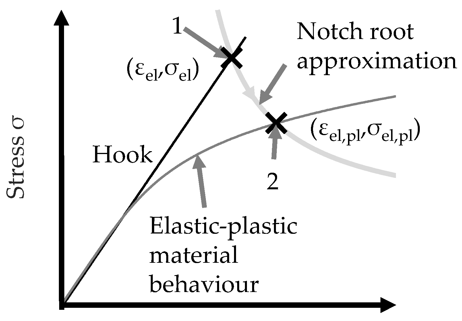
2. Notch Root Approximations in the FKM Guideline Nonlinear

Two different notch root approximations are available in the calculation algorithm of the FKM Guideline nonlinear:
  • Notch root approximation according to Neuber [27] in the variant according to [28].
  • Notch root approximation according to Seeger and Beste [30,31,32].
Both notch root approximations are used in the FKM Guideline nonlinear in such a way that they establish the relationship between a linear-elastically determined stress and the local elastic-plastic stresses and strains. The elastic-plastic stress state is thus estimated. This relationship between the linear-elastic stress and elastic-plastic stress is called the load-notch-strain curve of the component. This is used as a template with discrete values for the respective stresses in the Rainflow HCM algorithm [33] to simulate the path of the local stresses and strains depending on the path of the linear-elastic stress (load sequence) and to identify closed hysteresis loops. The HCM algorithm takes into account the effects of Masing’s behavior during load reversal [34] and material memory [1,33].
The FKM Guideline nonlinear uses the approach according to Ramberg and Osgood to describe the elastic-plastic material behavior [35].
ε el , pl = σ el , pl E + ( σ el , pl K ) 1 n
Here, E is Young’s modulus, K’ is the cyclic hardening coefficient, and n’ is the cyclic hardening exponent.
The determination of these parameters can be carried out either experimentally or by using estimation methods. For the evaluation of strain-controlled tests, the FKM Guideline nonlinear suggests a procedure based on [36] and [37]. In addition, a method developed by Wächter et al. [38,39] for the estimation of the cyclic properties using tensile strength is provided for use. This enables an analytical fatigue assessment to be carried out without the need for expensive experiments.
Using the cyclic parameters K’ and n’, it is possible to calculate a cyclic yield strength R’p0,2 as in Equation (4). R´p0,2 will later be of importance to estimate a maximum load.
R p 0.2 = 0.002 n K
For the material behavior on a hysteresis branch, the doubled curve applies with regard to stress and strain because of Masing’s behavior, illustrated in Figure 2:
Δ ε el , pl = Δ σ el , pl E + 2 · ( Δ σ el , pl 2 K ) 1 n
Due to this different behavior at the initial load and on load reversal, two load-notch-strain curves have to be determined. This can be performed before applying the HCM algorithm. In the FKM Guideline nonlinear, a total of 100 values with equally spaced intervals between the respective elasticity-theoretical values are specified for the discretization of the load-notch-strain curve for the initial load. According to Equation (5), the number of values for the hysteresis branch must be twice as large and amount to 200. The procedure is shown schematically for only eight values in Figure 3.
The load-notch-strain curves of the component for the initial load and for the hysteresis branch are related. It is possible to derive the initial load-notch-strain curve from the load-notch-strain curve of the hysteresis branch. By halving the values of elastic stress Δ σ el , elastic-plastic stress Δ σ el , pl , and elastic-plastic strain Δ ε el , pl range of every second of the abovementioned interval of the load-notch-strain-curve of the hysteresis branch, the initial load-notch-strain-curve is obtained. This is used in Section 4 and Section 5 to limit the investigation to the determination of the load-notch-strain-curve for the hysteresis branch.
For the application of both notch root approximations available in the FKM Guideline nonlinear, the knowledge of the limit load factor K p is necessary. The limit load factor describes the ratio of the external load L e , which leads to yielding at the local point under consideration, and the external load L p , which leads to global component collapse in the case of an elastic-ideal plastic material law, Equation (6). The limit load factor can either be approximately calculated by analytical relations for simple geometries [28,31,41] or, in the case of complex geometries, by FE analyses using elastic-ideal plastic material behavior. More details on the determination of Kp can be found in [28]. The limit load factor is assumed to be given from this point on.
K p = L p L e
At first glance, it may seem questionable to perform a notch root approximation if results from an elastic-plastic FE analysis are necessary for its application. However, it should be pointed out that the FE calculation is only needed to determine the load L p leading to plastic collapse. For this purpose, a much coarser FE mesh can be used compared to what would be necessary for the calculation of precise stress and strain values. In addition, K p is calculated with elastic-ideal-plastic material behavior. Both lead to significantly less calculation effort than when calculating the load-notch-strain curve using FE analysis with the Ramberg-Osgood material behavior.

2.1. Extended Version of Neuber’s Rule

The original version of Neuber’s rule [27] postulates, assuming elastic net-section behavior, the equality of the products of stress and strain for linear-elastic and elastic-plastic material behavior, Equation (7):
σ el , pl     ε el , pl = σ el     ε el
As shown by Seeger et al. [28,30,31,32] but also noted by Ellyin and Kujawski [42], this equation must be modified to account for high loads. To take into account the increasing net-section plasticity, Seeger and Heuler proposed a modification of the Neuber equation from Equation (7):
σ el , pl ε el , pl = σ el ε el * K p
The use of ε el * K p modifies the linear-elastic material behavior so that on the one hand, the real material behavior and on the other hand, the increasing net-section plasticity are taken into account [28,40]. The net section plasticity is modelled by ε el * using fictitious nominal stresses, obtained by means of the linear-elastic local stress σ el and the limit load factor K p , and inserting these into the material law. In this case the Ramberg and Osgood Equation (3) approach is used.
ε el * = σ el /   K p E + ( σ el /   K p K ) 1 / n
As mentioned above the load-notch-strain curve for initial load can be derived from the load-notch-strain curve of the hysteresis branch. Therefore, in the following only the procedure and the root finding equations for the hysteresis branch are explained. The detailed derivation, which also includes the formulas for the initial load curve, is shown in Appendix A. Equation (8) applied to the hysteresis branch can be transformed, as described above, into the root finding problem specified in the FKM Guideline nonlinear Equation (10).
f ( Δ σ el , pl ) = 0 = Δ σ el , pl E + 2     ( Δ σ el , pl 2 K ) 1 / n   ( Δ σ el Δ σ el , pl K p ( Δ σ el / K p E + 2 ( Δ σ el / K p 2 K ) 1 / n ) )
Equation (10) has to be solved for the 200 discrete required load steps of the load-notch-strain curves, respectively. The FKM Guideline nonlinear specifies Newton’s method for this purpose. (Other solution methods would also be possible, but since this paper focuses on the FKM Guideline nonlinear, only Newton’s method will be investigated, as specified).
Newton’s method is a numerical solution method in which, starting from an initial value x 0 , the following iteration (iteration step n) is executed up to a termination criterion:
x n + 1 = x n f ( x n ) f ( x n )
The objective is to find the root of the function f(x).
In the FKM Guideline nonlinear [25], the start values of iterations Δ σ 0 are defined to be the corresponding elasticity-theoretical solutions Δ σ el . The iteration is terminated after a fixed number of ten steps.
To apply Newton’s method, Equation (11), the user must first determine the derivatives f’ of the function f from Equation (10).
With the value for the stresses Δ σ el , pl determined in this way, the corresponding strain value can be calculated using Equation (5).

2.2. Notch Root Approximation according to Seeger and Beste

In addition to the extended version of Neuber’s rule, the notch root approximation of Seeger and Beste [30,31,32] is utilized in [25]. The relationship applied in this case is shown in Equations (12) and (13).
ε el , pl = σ el , pl E [ ( σ el σ el , pl ) 2 2 u 2 ln ( 1 cos ( u ) ) σ el σ el , pl + 1 ] ( ε el * E K p σ el )
with
u = π 2 ( ( σ el / σ el , pl )     1 K p     1 )
The resulting root finding problem specified in the FKM Guideline nonlinear for the hysteresis branch is shown in Equations (14)–(16).
f ( Δ σ el , pl ) = 0 = ( Δ σ el , pl E + 2 ( Δ σ el , pl 2 K ) 1 / n ) Δ σ el , pl E [ ( Δ σ el Δ σ el , pl ) 2 2 Δ u 2 ln ( 1 cos ( Δ u ) ) Δ σ el Δ σ el , pl + 1 ] ( Δ ε el * E K p Δ σ el )
with
Δ u = π 2 ( ( Δ σ el / Δ σ el , pl ) 1 K p 1 )
and
Δ ε el   * = Δ σ el /   K p E + 2 ( Δ σ el /   K p 2 K ) 1 / n
for the application of Newton’s method, a starting value is required. However, when considering the division term Δ u , it is noticeable that the starting value for the Newton iteration cannot be the linearly elastically determined stress, as described in Section 2.1, since the quotient Δ σ el / Δ σ el , pl   = 1 and thus the division term Δ u = 0 would follow. As a result, the undefined division by 0 would have to be carried out. Therefore, in [25], it is suggested to set the initial value Δ σ 0 slightly lower depending on the limit load factor K p according to Equation (17)
Δ σ 0 = Δ σ el ( 1   1 1 / K p 1000 )
analogous to the notch root approximation according to Neuber (Section 2.1), Newton’s method and the termination criterion of 10 iteration steps are specified in [25] to solve Equations (14)–(16).

3. Issues concerning the Implementation of Notch Root Approximations

When implementing the two notch root approximations presented above in the fatigue strength assessment in accordance with [25], the following questions arise for the user:
  • Is the formulation of the root finding problem a good option to ensure consistent accuracy over the entire load range?
  • How can the derivative f’ of the functions for the notch root approximation used in Newton’s method be obtained? Is it better to perform the derivation analytically or numerically?
  • Is the termination criterion specified in [25] for Newton’s method with a fixed number of 10 iterations suitable for reliably performing the notch root approximations? As alternative termination criteria, criteria based on an accuracy value could also be considered, which would lead to a variable number of iterations.
  • Are there other aspects to be considered with regard to a (numerically) stable and reliable implementation?
The following paragraphs first present proposed solutions for the mentioned aspects. These are later evaluated in Section 4 with regard to their effects on accuracy and efficiency.

3.1. Formulation of the Root Finding Problem for Use in Newton’s Method

In Section 2, the formulation of the root finding problem was described in the form defined in [25]. The disadvantage of this formulation is that it optimizes the difference of the strain (or strain range) ε el , pl , RO calculated with the material behavior according to Ramberg and Osgood (index RO) and ε el , pl , NRA calculated with the notch root approximation (index NRA) Equation (18).
f ( σ el , pl ) = 0 = ε el , pl , RO ( σ el , pl )     ε el , pl , NRA ( σ el , pl )
However, the underlying issue is that stresses and strains may be spread over several orders of magnitude, e.g., 1 MPa to 1000 MPa. In such a case, optimization of a difference leads to a situation where the relative error at the end of the iterations is dependent on the load level. It is thus considered reasonable to optimize on a factor so that a constant relative accuracy is ensured over all orders of magnitude.
Therefore, as a possible alternative, a formulation will be suggested here in which the factor between the resulting strain according to Equations (3)–(5), and the resulting strain from the notch root approximation is formed, Equation (19).
f ( σ el , pl ) = 0 = ε el , pl , RO ( σ el , pl ) ε el , pl , NRA ( σ el , pl ) 1
For the case of the extended Neuber’s rule, Equation (20) is the result for the hysteresis branch.
f ( Δ σ el , pl ) = 0 = Δ σ el , pl E + 2 ( Δ σ el , pl 2 K ) 1 / n Δ σ el Δ σ el , pl K p ( Δ σ el / K p E + 2 ( Δ σ el / K p 2 K ) 1 / n ) 1
For the notch root approximation according to Seeger and Beste, the formulation via quotient results in Equation (21) for the hysteresis branch.
f ( Δ σ el , pl ) = 0 = Δ σ el , pl E + 2 ( Δ σ el , pl 2 K ) 1 / n Δ σ el , pl E [ ( Δ σ el Δ σ el , pl ) 2 2 Δ u 2 ln ( 1 cos ( Δ u ) ) Δ σ el Δ σ el , pl + 1 ] Δ ε el * E K p Δ σ el 1
using Δ u from Equation (15) and Δ ε el * from Equation (16).

3.2. Derivatives of the Functions for Use in Newton’s Method

To apply Newton’s method, not only the functions for the root finding problem, i.e., Equations (10), (14)–(16), (20) and (21), are required but also their derivatives need to be known. In this section only the derivatives for the hysteresis branch formulations of the root finding problems will be discussed, the full list of derivatives are given in Appendix B.
In the case of the extended notch root approximation according to Neuber, the derivative of Equation (10) is relatively easy to determine analytically. It is given in Equation (22).
df d Δ σ el , pl = f ( Δ σ el , pl ) = 1 E + ( Δ σ el , pl 2 K ) 1 / n 1 K n + K p σ el ( 2 ( Δ σ el 2 K K p ) 1 / n + Δ σ el E K p ) Δ σ el , pl 2
The derivative for the alternative approach, Equation (20), described in the Section 3.1, is given in Equation (23).
df d Δ σ el , pl = f ( Δ σ el , pl ) = Δ σ el , pl E + 2 ( Δ σ el , pl 2 K ) 1 / n K p Δ σ el ( 2 ( Δ σ el 2 K K p ) 1 / n + Δ σ el E K p ) + Δ σ el , pl ( 1 E + ( Δ σ el , pl 2 K ) 1 / n 1 K n ) K p Δ σ el ( 2 ( Δ σ el 2 K K p ) 1 / n + Δ σ el E K p )
The notch root approximation according to Seeger and Beste has clearly more extensive expressions in the root finding problem, namely, Equations (14)–(16) and (21). In principle, the derivatives can also be determined analytically. However, practically, the analytical derivative can only be calculated using a computer algebra system (CAS). The derivative of Equation (14) is shown in Equation (24).
df d Δ σ el , pl = f ( Δ σ el , pl ) = 1 E + ( Δ σ el , pl K ) 1 / n 1 K n 1 Δ σ el ( K p Δ ε el * ( 8 Δ σ el 2 ln ( 1 cos ( Δ u ) ) ( K p 1 ) 2 Δ σ el , pl 2 π 2 ( Δ σ el Δ σ el , pl 1 ) 2 Δ σ el Δ σ el , pl + 1 ) ) + K p Δ ε el * Δ σ el , pl Δ σ el ( Δ σ el Δ σ el , pl 2 16 Δ σ el 2 ln ( 1 cos ( Δ u ) ) ( K p 1 ) 2 Δ σ el , pl 3 π 2 ( Δ σ el Δ σ el , pl 1 ) 2 + 16 Δ σ el 3 ln ( 1 cos ( Δ u ) ) ( K p 1 ) 2 Δ σ el , pl 4 π 2 ( Δ σ el Δ σ el , pl 1 ) 3 4 Δ σ el 3 sin ( Δ u ) ( K p 1 ) Δ σ el , pl 4 π cos ( Δ u ) ( Δ σ el Δ σ el , pl 1 ) 2 )
The derivative of Equation (21) is shown in Equation (25). It is noticeable that these equations are practically difficult to handle without error.
df d Δ σ el , pl = f ( Δ σ el , pl ) = Δ σ el ( 1 E + ( Δ σ el , pl 2 K ) 1 / n 1 K n ) K p Δ ε * Δ σ el , pl ( 8 Δ σ el , pl 2 ln ( 1 cos ( Δ u ) ) ( K p 1 ) 2 π 2 Δ σ el , pl 2 ( Δ σ el Δ σ el , pl 1 ) 2 Δ σ el Δ σ el , pl + 1 ) Δ σ el ( Δ σ el , pl E + 2 ( Δ σ el , pl 2 K ) 1 / n ) K p Δ ε * Δ σ el , pl 2 ( 8 Δ σ el 2 ln ( 1 cos ( Δ u ) ) ( K p 1 ) 2 π 2 Δ σ el , pl 2 ( Δ σ el Δ σ el , pl 1 ) 2 Δ σ el Δ σ el , pl + 1 ) 1 K p Δ ε * Δ σ el , pl ( 8 Δ σ el 2 ln ( 1 cos ( Δ u ) ) ( K p 1 ) 2 π 2 Δ σ el , pl 2 ( Δ σ el Δ σ el , pl 1 ) 2 Δ σ el Δ σ el , pl + 1 ) 2 Δ σ el ( Δ σ el , pl E + 2 ( Δ σ el , pl 2 K ) 1 / n ) ( Δ σ el Δ σ el , pl 2 16 Δ σ el 2 ln ( 1 cos ( Δ u ) ) ( K p 1 ) 2 π 2 Δ σ el , pl 3 ( Δ σ el Δ σ el , pl 1 ) 2 + 16 Δ σ el 3 ln ( 1 cos ( Δ u ) ) ( K p 1 ) 2 π 2 Δ σ el , pl 4 ( Δ σ el Δ σ el , pl 1 ) 3 4 Δ σ el 3 sin ( Δ u ) ( K p 1 ) π Δ σ el , pl 4 cos ( Δ u ) ( Δ σ el Δ σ el , pl 1 ) 2 )
Therefore, an alternative procedure will be discussed here. It is possible to approximate the derivative numerically via the difference quotient, whereby the central difference quotient is used here, Equation (26). Here, h is the step size, which is set to 0.0001.
f ( x 0 )     f ( x 0 + h ) f ( x 0 h ) 2 h

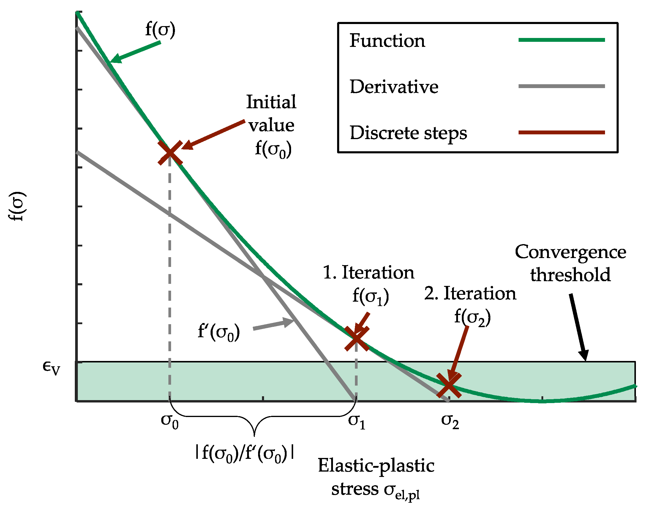
3.3. Termination Criteria for Newton’s Method

Numerical methods generate an infinite sequence of values if no termination criterion is defined. If correctly chosen, the termination criterion guarantees that the procedure is terminated after a finite number of steps. In general, the procedure is terminated if a desired accuracy of the solution is reached or if no solution can be found with the selected parameters. In the case of Newton’s method, the following variants are conceivable:
  • Termination after a predefined number of iterations.
  • Termination when the value of the root finding problem falls below ϵ V , i.e., when Equation (27) is fulfilled. This is the case if the function value of the root finding problem is sufficiently close to zero; compare Figure 4.
    f ( σ n )   <   ϵ V
In this paper, the following criteria are investigated in more detail:
  • Termination after 10 fixed steps, as suggested in [25].
  • Termination after falling below a function value f ( σ n )   <   ϵ V .
    • using f according to Equations (10) and (14) (i.e., finding the root of the difference of ε el , pl , RO ε el , pl , NRA ) and ϵ Vd   = 10 7 .
    • using f according to Equations (20) and (21) (i.e., finding the root of the quotient of ε el , pl , RO / ε el , pl , NRA 1 ) and ϵ Vq = 10 3 .
Variants 2a and 2b aim to reach a defined accuracy for the solution, while no prediction can be made about the required number of iterations. On the other hand, the number of iterations is fixed for variant 1, but no control of the calculation accuracy is provided.
The concrete threshold levels for termination criteria 2a and 2b were determined based on the following considerations:
  • A small remaining strain deviation in criterion 2a has a high influence, especially at low stresses.
    For example, for steel (Young’s modulus E     200 , 000   MPa ), a value of ϵ Vd = 10 7 leads to a deviation in the stress direction of 0.02 MPa at 1 MPa, which corresponds to a relative deviation of 2%.
    With increasing loads, the deviation of 0.02 MPa remains almost constant, so the relative error decreases.
    The maximum error is 2 % .
  • If the absolute deviation of 0.02 MPa from the previous point is now applied to a load height of 20 MPa, then the following value results for ϵ Vq for termination criterion 2b:
    ε f = ( 20   MPa / 200 , 000   MPa ) + 10 7 ( 20   MPa / 200 , 000   MPa ) = 1.001 or since in Equations (20) and (21), 1 is subtracted. The result is ϵ Vq = 10 3 .
Variants 2a and 2b are motivated by the assumption that Newton’s method with a quadratic order of convergence usually converges in 3 to 4 steps, meaning that it may not be necessary to use 10 steps in most cases, and therefore, on average, a performance gain might be achieved compared to variant 1, as proposed in [25].

3.4. Consideration of the Numerical Stability

In the case of the extended notch root approximation according to Neuber, no special considerations have to be made with regard to stability. In all variants considered in this paper, the solution via Newton’s method reacts insensitively to small interferences of the input data.
The calculation of the notch root approximation according to Seeger and Beste, on the other hand, can result in complex numerical values, regardless of whether the analytical derivation or the numerical approximation is used. Complex values become possible in the context if, for example, the term ln(1/cos(u)), see Equation (12), becomes negative. This always seems to occur when a comparatively large number of Newton iterations are carried out, i.e., using the termination after 10 fixed steps. However, using termination criteria 2a and 2b, the condition for termination is always reached before complex values occur. A specific formula for determining when complex numbers are to be expected cannot be provided. The example in Table 1 demonstrates that a small rounding error can lead to unstable behavior. In this example, a small change in the 9th decimal place of the elastic stress range Δ σ el can lead to this unstable behavior and thus to complex values. This example is taken from the study described in the next section and thus represents a case that can also occur in this way in practical applications.

4. Evaluation of Performance and Accuracy of Different Implementations

The described options in Section 3 regarding the implementation of the two notch root approximations are to be evaluated in terms of the following two aspects:
  • The accuracy with which the notch root approximations are carried out affects the results of the fatigue strength assessment.
  • The calculation resources required for the application or the required computing time matter for an efficient implementation. When performing single calculations on a single or a few individual locations of a component to be verified, this aspect is not important. However, in regard to performing many assessments, e.g., when applied to a whole FE surface mesh of a component, the calculation time becomes a decisive factor.
For this purpose, a large number of artificial examples are considered in the following, which contain all necessary input variables for a notch root approximation with the two notch root approximations described above. For these examples, notch root approximations are performed with the different implementation variants, and the calculation results of the different variants are compared with each other in terms of accuracy and efficiency.

4.1. Database

For the following evaluation of calculation quality and efficiency, a database with 10 fictitious example geometries, each with 100 different configurations for the cyclic properties, is used. These example geometries are represented by one dataset containing all required input values for the two notch root approximations specified in [25]. These are as follows:
  • Maximum linear-elastic stress range relevant for the strength verification Δ σ el , max .
  • Tensile strength Rm for estimation of Ramberg-Osgood parameters according to [25].
  • Limit load factor Kp.
These input values are defined within the value ranges given in Table 2.
The tensile strength R m varies within a large range, representing the range of validity within the FKM Guideline nonlinear [25] for the steel material group and is used to estimate the cyclic material properties by applying the method from [25]. The limit load factor is varied within a range that is assumed to be relevant in practice. The maximum load is based on the cyclic yield strength, which can be determined using Equation (4), and the limit load factor, which, as already mentioned, is a measure of the maximum load that can be applied.
The dataset is constructed as follows: Every possible permutation consisting of the first two rows of Table 2 is generated. Then, for each combination, the cyclic material properties shown in Rows 3 to 5 are estimated. Next, the maximum linear-elastic stress ranges are determined based on the cyclic material properties in the range given in Table 2. Finally, for each of these combinations, notch root approximations on the hysteresis branch (since, as mentioned in Section 2, the initial load-notch-strain curve can be estimated from the load-notch-strain curve of the hysteresis branch) are performed according to [25] with 200 discrete points. In summary, this leads to ~20,000,000 data points and notch root approximations.

4.2. Implementation into Software Code

To evaluate the abovementioned different variants of the notch root approximation implementation, two different programming languages are utilized:
  • The software environment MATLAB (version 2020b) was used to represent script languages and
  • Fortran (Intel Ifort 2019 Update 5 using “-O3” optimization) was used to represent compiled languages in machine code.
Script languages and compiled programming languages can be optimized differently for the respective calculation tasks. This in turn can lead to situations where a termination criterion for the Newton iteration, which results in high performance in one case, is not optimal in the other case. For this reason, both of the abovementioned programming languages were used for this study.
All calculations were carried out separately for the variants of the termination criteria. For the notch root approximation of Seeger and Beste, in addition to the termination criterion, the type of derivation (analytical derivation according to Equations (24) and (25) or numerical approximation according to Equation (26)) is also varied here. Therefore, the following nine variants are investigated:
  • Enhanced Neuber using the analytical derivative and termination after 10 fixed steps
  • Enhanced Neuber using the analytical derivative, termination if Equation (10) falls below ϵ Vd = 10 7
  • Enhanced Neuber using the analytical derivative, termination if Equation (20) falls below ϵ Vq = 10 3
  • Seeger/Beste using the analytical derivative, termination after 10 fixed steps
  • Seeger/Beste using the analytical derivative, termination if Equation (14) falls below ϵ Vd = 10 7
  • Seeger/Beste using the analytical derivative, termination if Equation (21) falls below ϵ Vq = 10 3
  • Seeger/Beste using the numerical approximation of the derivative, termination after 10 fixed steps
  • Seeger/Beste using the numerical approximation of the derivative, termination if Equation (14) falls below ϵ Vd = 10 7
  • Seeger/Beste using the numerical approximation of the derivative, termination if Equation (21) falls below ϵ Vq = 10 3

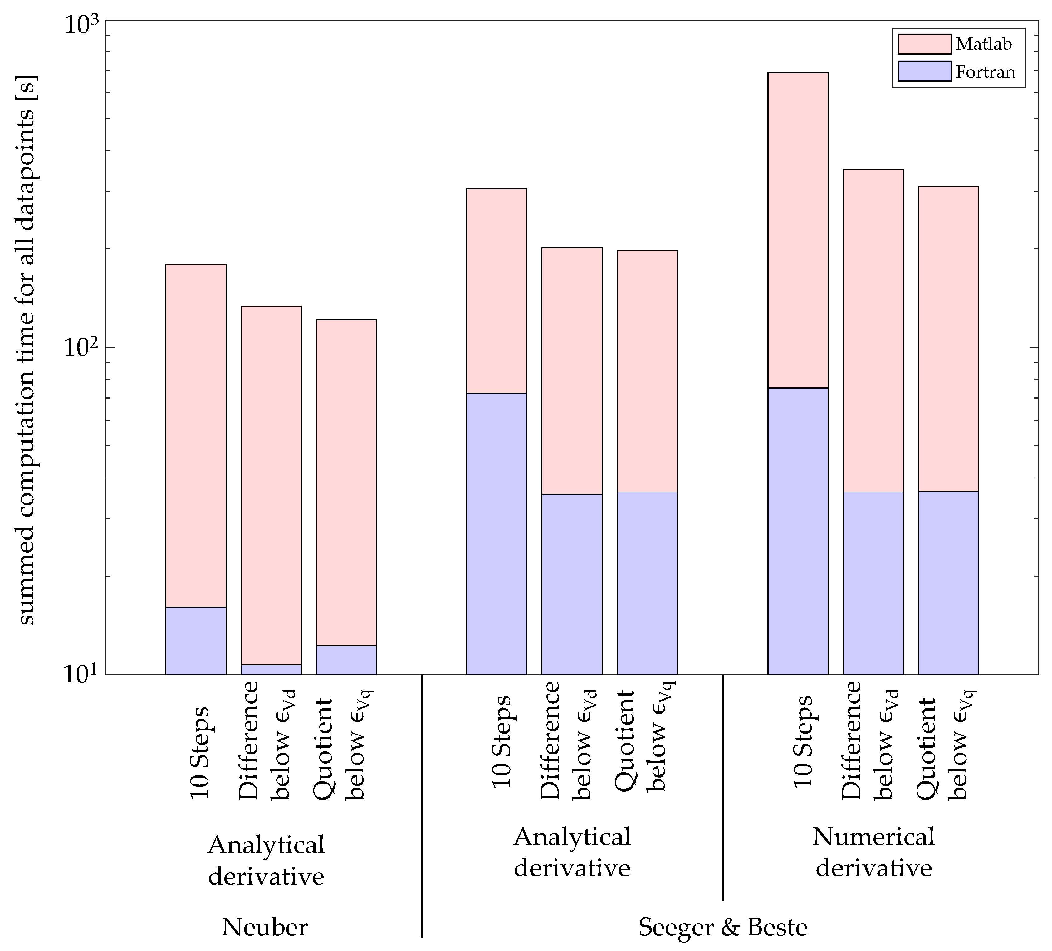
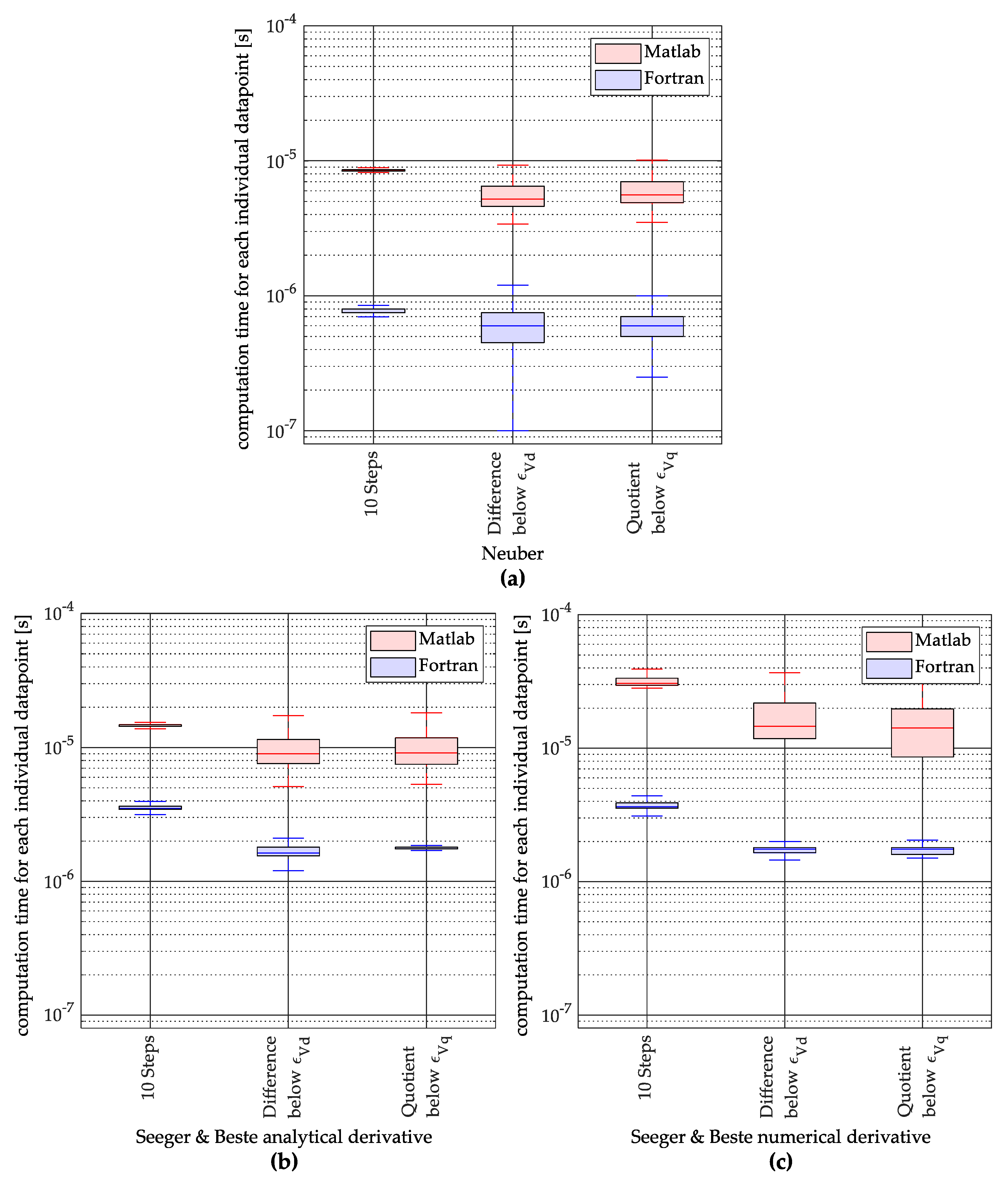
4.3. Results and Discussion

The database described in Section 4.1 is used to investigate the performance of the abovementioned variants. For each dataset, the notch root approximations of each of the nine variants 1 through 9 (Section 4.2) are executed using both MATLAB and Fortran implementations.
For a qualitative comparison of the individual variants, two calculation runs are performed. In the first calculation run, the number of Newton iterations until convergence is recorded (which is independent from the programming language used). The distribution of the number of iterations is shown in Figure 5. The boxes graphically represent the 25% and 75% quantiles of the required number of Newton iteration steps to converge. In other words, 50% of all points are inside the box. The whiskers represent the minimum and maximum values of iteration steps ignoring outliers.
The distribution of the number of iterations required until the termination criteria are met is independent of whether the analytical derivation or the numerical approximation is used. For this reason, Figure 5b shows the distribution of the required Newton steps independent of the method of derivation.
Figure 5a,b show that for termination criteria where an accuracy is specified, almost always less than 10 Newton steps are required. In some cases, i.e., when applying low loads, the termination criteria are fulfilled before the iteration starts. At the same time, it should be noted that in a few cases, when using a criterion quotient below ϵ Vq , more than 10 steps are required to achieve the desired accuracy.
In a second calculation run, only the calculation times are recorded. The resulting summed calculation time obtained by performing the extended version of Neuber’s rule on the ~20,000,000 data points, carried out on an Intel i5-8400H CPU, is on the order of 120–180 s when using MATLAB and 10–15 s when using Fortran. In the case of the MATLAB script, the overall fastest variant for the extended version of the Neuber rule is termination when Equation (20) (meaning the quotient of ε el , pl , RO / ε el , pl , NRA converges) reaches the desired accuracy. In case of the Fortran program the fastest variant is Equation (10) (difference ε el , pl , RO ε el , pl , NRA ) falls below ϵVd.
In the case of the notch root approximation of Seeger and Beste, the summed calculation time is on the order of 200–300 s when using MATLAB. In the Fortran program, the summed calculation time is on the order of 35–70 s. As in the case of the extended version of Neuber’s rule, Equation (21) (quotient ε el , pl , RO / ε el , pl , NRA ) is the fastest approach when using MATLAB, and Equation (14) (difference ε el , pl , RO ε el , pl , NRA ) is the fastest approach when using Fortran.
The summed calculation times and the abovementioned findings are shown graphically in Figure 6.
The distribution of the individual calculation times for each data point is shown in Figure 7. The calculation times for the extended version of Neuber’s rule are shown in Figure 7a. It can be seen that the termination after reaching a desired accuracy results in shorter calculation times on average compared to the 10-step approach.
The calculation times for the Seeger and Beste approach are shown in Figure 7b using the analytical derivation and in Figure 7c using the numerical approximation. As with Neuber’s rule, the approaches using a desired accuracy lead to faster calculations compared to the 10-step approach. This influence is greater in the implementation in Fortran by a factor of 2.5 than in MATLAB (Factor 2).
Using Figure 7b,c, the two approaches for the derivation can also be compared with regard to the computing time. Notably, in the case of the implementation in MATLAB, the approximate method for the derivative via the difference quotient leads to higher calculation times with the same termination criterion, while in Fortran, no significant influence is visible.
One attempt at an explanation is based on Fortran’s high degree of optimization. The recorded calculation times in Fortran are so short that other effects, such as background tasks in the operating system, have a greater influence than the actual calculations.
Considering that the numerical derivative from Equation (26) is significantly easier to handle than the analytical derivation from Equations (24) and (25), it can be concluded that for the notch root approximations according to Seeger and Beste, the numerical derivative in combination with the termination criterion 2a or 2b is a practical choice.
The deviations of the estimated stresses of all variants in comparison to each other are on the order of 10 7 MPa. Deviations of this order of magnitude have a negligible influence on the calculated service life estimation.
It can therefore be concluded that for both notch root approximations in question, termination criteria using a specific accuracy significantly reduces the number of necessary Newton iterations and improves the computational performance compared to the 10-step termination criterion proposed in the FKM Guideline nonlinear [25]. At the same time, the resulting stresses and strains are not significantly influenced.

5. Conclusions

In this paper, the theoretical background of notch root approximations is reviewed as far as it is necessary for practical implementation in the FKM Guideline nonlinear [25]. The application of notch root approximations requires the solution of a nonlinear equation. This solution is usually performed using Newton’s method. The implementation of this method is the subject of this paper. In this context, the aspects of stability, performance, formulation of the root finding problem and accuracy are considered in more detail. This is interesting, for example, if the notch root approximation is to be applied to each node in the scope of variant calculations or in a postprocessing of a linear-elastic FE analysis.
The FKM Guideline nonlinear uses the extended Neuber’s rule and the notch root approximation according to Seeger and Beste. Both were examined more closely in this paper with regard to the aspects mentioned above. The results obtained show that (not depending on the notch root approximation method):
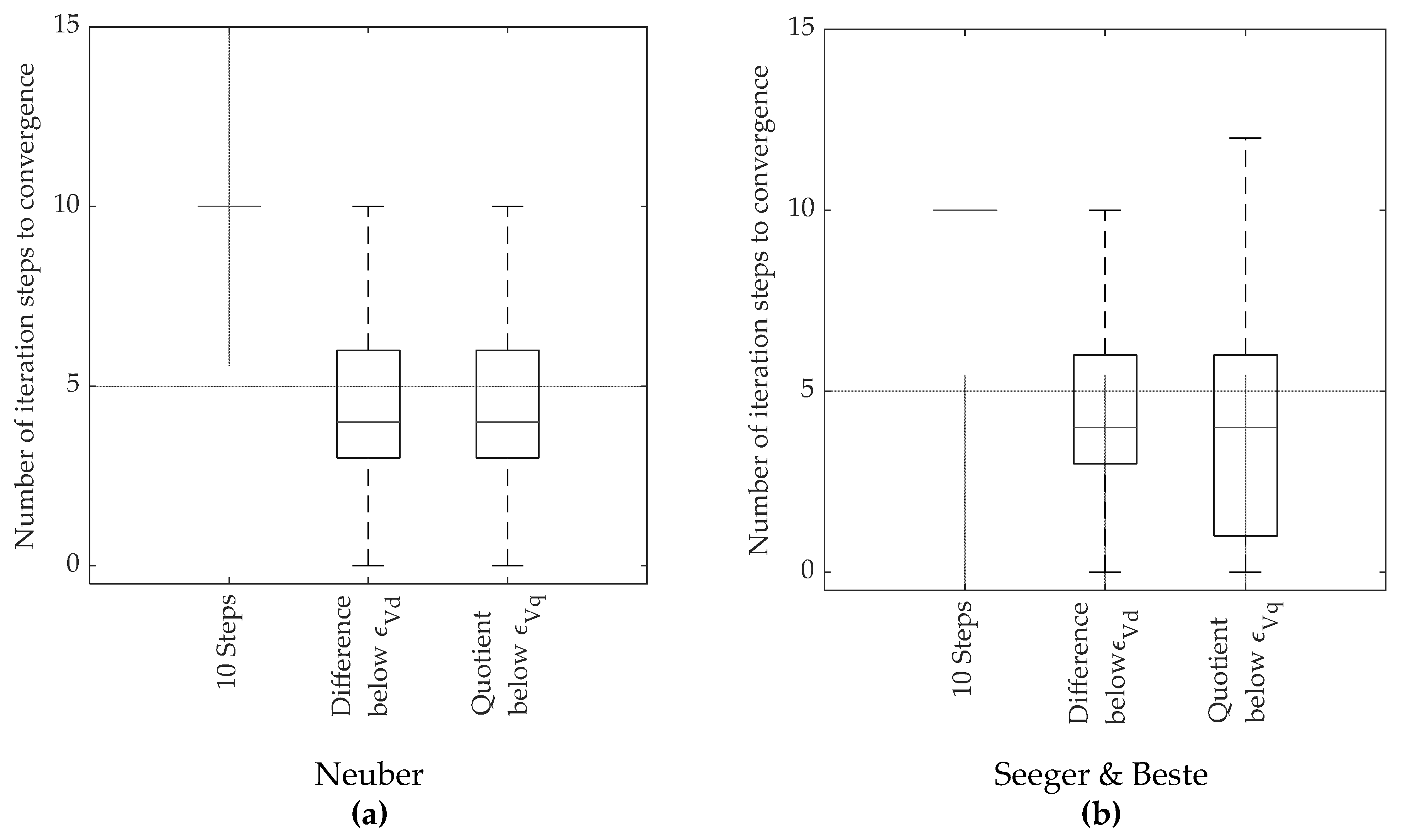
  • 10 Newton steps, as suggested in [25], almost always lead to a desired accuracy but are not required in most cases.
  • In the case of a script language, here represented by MATLAB, the formulation of the root finding problem in the form of a quotient between the strain calculated via the material law and the strain calculated via the notch root approximation leads to the best computational performance.
  • In the case of a language compiled in machine code, here represented by Fortran, the formulation of the root finding problem in the form of a difference in the strain calculated via the material law and strain calculated via the notch root approximation leads to the best computational performance.
In particular, for the notch root approximation according to Seeger and Beste, the following findings were also obtained:
  • If Seeger and Beste’s notch root approximations are used and an incorrect termination criterion is selected, then there is a risk that the automated calculation will produce complex numbers that cannot be interpreted meaningfully in terms of a service life calculation. Here, the use of the termination criteria with a desired accuracy leads to the most stable solution, in the sense that no complex number arose in the examined parameter field.
  • The analytical derivative of the notch root approximation according to Seeger and Beste cannot be trivially used. The numerical approximation via the difference quotient is much easier to handle and leads to minor losses in performance when used in MATLAB and to comparable performance when used in Fortran.
For implementation in engineering practice, the overall recommendation for both notch approximation methods considered here is therefore to use the termination criterion where the quotient of the strain ε el , pl , RO / ε el , pl , NRA converges, which leads to a constant relative accuracy over all orders of magnitude, especially when using a script language. The source code implementing all considered variants in this study are provided as a reference implementation in [43].

Author Contributions

Conceptualization, R.B., L.M., M.W. and A.E.; methodology, R.B. and M.W.; software, R.B.; validation, L.M., M.W. and A.E.; investigation, R.B.; resources, L.M.; writing—original draft preparation, R.B.; writing—review and editing, M.W., L.M. and A.E.; visualization, R.B. and M.W.; supervision, A.E.; project administration, M.W. and A.E. All authors have read and agreed to the published version of the manuscript.

Funding

This research received no external funding. However, we acknowledge support from the Open Access Publishing Fund of Clausthal University of Technology.

Data Availability Statement

The source code implementing all considered variants in this study is openly available as MATLAB source in [43].

Conflicts of Interest

The authors declare no conflict of interest.

Nomenclature

EYoung’s modulus
F function placeholder of the root finding problem
f’function placeholder of the derivative of the root finding problem
FEfinite element
FKMAbbreviation for the german research association “Forschungskuratorium Maschinenbau”
Hstep size
kmean stress correction factor
K cyclic hardening coefficient
K p limit load factor
L e reference load for local yielding
L p reference load for plastic collapse
n cyclic hardening exponent
NRAnotch root approximation
PRAJload parameter
PRAMload parameter
R p 0.2 cyclic yield strength
RORamberg Osgood
Δ range of stress/strain of a hysteresis
Δ ε eff effective elastic-plastic strain range
Δ σ eff effective elastic-plastic stress range
ε a strain amplitude of the detected stress-strain hysteresis
ε el linear-elastic local strain
ε el * substitution strain for net section plasticity
ε el , pl elastic-plastic local strain
ϵ V placeholder for the convergence threshold
ϵ Vd convergence threshold when finding the root of the difference
ϵ Vq convergence threshold when finding the root of the quotient
σ 0 start value of elastic-plastic stress for the newton iteration
σ a stress amplitude of the detected stress-strain hysteresis
σ el linear-elastic local stress
σ el , pl elastic-plastic local stress
σ m mean stress of the detected stress-strain hysteresis
σ n value of elastic-plastic stress in the n-th newton iteration

Appendix A. Derivation of the Root Finding Equations

In this section the derivation of the different root finding equations shall be described in more detail. Here, the derivation in which the difference of ε el , pl , RO according to Ramberg and Osgood and ε el , pl , NRA according to the notch root approximation is minimised takes place first, followed by the derivation in which the quotient of both strains is minimised. The procedure is always demonstrated using the extended version of Neuber’s rule first and then the results for the method according to Seeger and Beste are shown.

Appendix A.1. Root Finding Equations Formulated by Taking the Difference

The starting point is the extended version of the Neuber’s rule:
σ el , pl ε el , pl   = σ el ε el * K p
In a first step ε el * , which considers the material behavior in case net section plasticity takes place, needs to be replaced with the material behavior according to Ramberg and Osgood:
σ el , pl ε el , pl = σ el K p ( σ el / K p E + ( σ el / K p K ) 1 / n )
Equation (A2) may be rearranged to:
ε el , pl = σ el σ el , pl K p ( σ el / K p E + ( σ el / K p K ) 1 / n )
In order to obtain a unique solution for the stress and strain, a second equation is required. As the FKM Guideline nonlinear uses Ramberg and Osgood material behavior ε el , pl from (A3) can be replaced with Equation (3):
σ el , pl E + ( σ el , pl K ) 1 / n = σ el σ el , pl K p ( σ el / K p E + ( σ el / K p K ) 1 / n )
The next step is to solve this equation for the desired elastic plastic stress. For this purpose, the equation is converted into a root-finding problem by taking the difference of the strains.
0 = σ el , pl E + ( σ el , pl K ) 1 / n σ el σ el , pl K p ( σ el / K p E + ( σ el / K p K ) 1 / n )
The steps described above can be applied for the hysteresis branch in the same way. In this case Equation (A6) results:
0 = Δ σ el , pl E + 2 ( Δ σ el , pl 2 K ) 1 / n Δ σ el Δ σ el , pl K p ( Δ σ el / K p E + 2 ( Δ σ el / K p 2 K ) 1 / n )
Next, the identical procedure will be applied to the approach according to Seeger and Beste Equations (A7)–(A9).
ε el , pl = σ el , pl E [ ( σ el σ el , pl ) 2 2 u 2 ln ( 1 cos ( u ) ) σ el σ el , pl + 1 ] ( ε el * E K p σ el )
with
u = π 2 ( ( σ el / σ el , pl ) 1 K p 1 )
and
ε el * = σ el /   K p E + ( σ el /   K p K ) 1 / n
Equation (A7) (including (A8) and (A9)) is now equated with Equation (3).
σ el , pl E + ( σ el , pl K ) 1 / n = σ el , pl E [ ( σ el σ el , pl ) 2 2 u 2 ln ( 1 cos ( u ) ) σ el σ el , pl + 1 ] ( ε el * E K p σ el )
Rearranging the equation as already demonstrated for Neuber’s rule also leads here to the difference formulation of the root finding problem.
0 = σ el , pl E + ( σ el , pl K ) 1 / n σ el , pl E [ ( σ el σ el , pl ) 2 2 u 2 ln ( 1 cos ( u ) ) σ el σ el , pl + 1 ] ( ε el * E K p σ el )
In the case of calculating a hysteresis branch Equation (A12) results:
0 = Δ σ el , pl E + 2 ( Δ σ el , pl 2 K ) 1 / n Δ σ el , pl E [ ( Δ σ el Δ σ el , pl ) 2 2 Δ u 2 ln ( 1 cos ( Δ u ) ) Δ σ el Δ σ el , pl + 1 ] ( Δ ε el * E K p Δ σ el )
with
Δ u = π 2 ( ( Δ σ el / Δ σ el , pl )     1 K p 1 )
and
Δ ε el * = Δ σ el /   K p E + 2 ( Δ σ el /   K p 2 K ) 1 / n

Appendix A.2. Root Finding Equations Formulated by Taking the Quotient

Instead of forming the difference between the strain from the material law and the strain from the notch root approximation, the quotient can also be formed and converted into a zero-point formulation. In the case of the extended version of Neuber’s rule, starting from Equation (A4), the quotient can now be formed as follows.
1 = σ el , pl E + ( σ el , pl K ) 1 / n σ el σ el , pl K p ( σ el / K p E + ( σ el / K p K ) 1 / n )
To obtain the root finding equation one has to subtract 1.
0 = σ el , pl E + ( σ el , pl K ) 1 / n σ el σ el , pl K p ( σ el / K p E + ( σ el / K p K ) 1 / n ) 1
The above steps can be applied in the same way for the hysteresis branch. In this case Equation (A17) results:
  0 = Δ σ el , pl E + 2 ( Δ σ el , pl 2 K ) 1 / n Δ σ el Δ σ el , pl K p ( Δ σ el / K p E + 2 ( Δ σ el / K p 2 K ) 1 / n )     1
Transferred to the method according to Seeger and Beste, we obtain for the initial load curve
0 = σ el , pl E + ( σ el , pl K ) 1 / n σ el , pl E [ ( σ el σ el , pl ) 2 2 u 2 ln ( 1 cos ( u ) ) σ el σ el , pl + 1 ] ε el * E K p σ el     1
and for the hysteresis branch Equation (A19)
0 = Δ σ el , pl E + 2 ( Δ σ el , pl 2 K ) 1 / n Δ σ el , pl E [ ( Δ σ el Δ σ el , pl ) 2 2 Δ u 2 ln ( 1 cos ( Δ u ) ) Δ σ el Δ σ el , pl + 1 ] Δ ε el * E K p Δ σ el 1

Appendix B. Derivatives of the Root Finding Equations

In this section the analytical derivatives of the different root finding equations, derived in the Appendix A are listed.
In the case of the extended notch root approximation according to Neuber, the derivatives of Equation (A5) (initial load curve) and Equation (A6) (hysteresis branch) are given in Equations (A20) and (A21).
f ( σ el , pl ) = 1 E + ( σ el , pl K ) 1 / n 1 K n + K p σ el ( ( σ el K K p ) 1 / n + σ el E K p ) σ el , pl 2
f ( Δ σ el , pl ) = 1 E + ( Δ σ el , pl 2 K ) 1 / n 1 K n + K p σ el ( 2 ( Δ σ el 2 K K p ) 1 / n + Δ σ el E K p ) Δ σ el , pl 2  
The derivatives for the alternative approach, i.e., Equation (A16) (initial load curve) and Equation (A17) are given in Equations (A22) and (A23).
f ( σ el , pl ) = σ el , pl E + ( σ el , pl K ) 1 / n K p σ el ( ( σ el K K p ) 1 / n + σ el E K p ) + σ el , pl ( 1 E + ( σ el , pl K ) 1 / n 1 K n ) K p σ el ( ( σ el K K p ) 1 / n + σ el E K p )  
f ( Δ σ el , pl ) = Δ σ el , pl E + 2 ( Δ σ el , pl 2 K ) 1 / n K p Δ σ el ( 2 ( Δ σ el 2 K K p ) 1 / n + Δ σ el E K p ) + Δ σ el , pl ( 1 E + ( Δ σ el , pl 2 K ) 1 / n 1 K n ) K p Δ σ el ( 2 ( Δ σ el 2 K K p ) 1 / n + Δ σ el E K p )
In case of the notch root approximation according to Seeger and Beste the derivative of the difference formulation of the root finding equation Equation (A11) (initial load curve) is shown in Equation (A24) and the derivative of Equation (A12) (hysteresis branch curve) in Equation (A25).
df d σ el , pl = f ( σ el , pl ) = 1 E + ( σ el , pl K ) 1 / n 1 K n     1 σ el ( K p ε el * ( 8 σ el 2 ln ( 1 cos ( u ) )   ( K p 1 ) 2 σ el , pl 2 π 2 ( σ el σ el , pl 1 ) 2 σ el σ el , pl + 1 ) ) K p ε el * σ el , pl σ el ( σ el σ el , pl 2 16 σ el 2 ln ( 1 cos ( u ) ) ( K p 1 ) 2 σ el , pl 3 π 2 ( σ el σ el , pl 1 ) 2 + 16 σ el 3 ln ( 1 cos ( u ) ) ( K p 1 ) 2 σ el , pl 4 π 2 ( σ el σ el , pl 1 ) 3 4 σ el 3 sin ( u ) ( K p 1 ) σ el , pl 4 π cos ( u ) ( σ el σ el , pl 1 ) 2 )
df d Δ σ el , pl = f ( Δ σ el , pl ) = 1 E + ( Δ σ el , pl K ) 1 / n 1 K n 1 Δ σ el ( K p Δ ε el * ( 8 Δ σ el 2 ln ( 1 cos ( Δ u ) ) ( K p 1 ) 2 Δ σ el , pl 2 π 2 ( Δ σ el Δ σ el , pl 1 ) 2 Δ σ el Δ σ el , pl + 1 ) ) + K p Δ ε el * Δ σ el , pl Δ σ el ( Δ σ el Δ σ el , pl 2 16 Δ σ el 2 ln ( 1 cos ( Δ u ) ) ( K p 1 ) 2 Δ σ el , pl 3 π 2 ( Δ σ el Δ σ el , pl 1 ) 2 + 16 Δ σ el 3 ln ( 1 cos ( Δ u ) ) ( K p 1 ) 2 Δ σ el , pl 4 π 2 ( Δ σ el Δ σ el , pl 1 ) 3 4 Δ σ el 3 sin ( Δ u ) ( K p 1 ) Δ σ el , pl 4 π cos ( Δ u ) ( Δ σ el Δ σ el , pl 1 ) 2 )
In case of the notch root approximation according to Seeger and Beste the derivative of the quotient formulation of the root finding problem Equation (A18) (initial load curve) is shown in Equation (A26) and of Equation (A19) (hysteresis branch curve and quotient formulation) in Equation (A27).
df d σ el , pl = f ( σ el , pl ) = σ el ( 1 E + ( σ el , pl K ) 1 / n 1 K n ) K p ε el * σ el , pl ( 8 σ el 2 ln ( 1 cos ( u ) ) ( K p 1 ) 2 σ 2 π 2 ( σ el σ el , pl 1 ) 2 σ el σ el , pl + 1 ) σ el ( σ el , pl E + ( σ el , pl K ) 1 / n ) K p ε el * σ el , pl 2 ( 8 σ el 2 ln ( 1 cos ( u ) ) ( K p 1 ) 2 σ el , pl 2 π 2 ( σ el σ el , pl 1 ) 2 σ el σ el , pl + 1 ) 1 K p ε el * σ el , pl ( 8 σ el 2 ln ( 1 cos ( u ) ) ( K p 1 ) 2 σ el , pl 2 π 2 ( σ el σ el , pl 1 ) 2 σ el σ el , pl + 1 ) 2 σ el ( σ el , pl E + ( σ el , pl K ) 1 / n ) ( σ el σ el , pl 2 16 σ el 2 ln ( 1 cos ( u ) ) ( K p 1 ) 2 σ el , pl 3 π 2 ( σ el σ el , pl 1 ) 2 + 16 σ el 3 ln ( 1 cos ( u ) ) ( K p 1 ) 2 σ el , pl 4 π 2 ( σ el σ el , pl 1 ) 3 4 σ el 3 sin ( u ) ( K p 1 ) σ el , pl 4 π cos ( u ) ( σ el σ el , pl 1 ) 2 )
df d Δ σ el , pl = f ( Δ σ el , pl ) = Δ σ el ( 1 E + ( Δ σ el , pl 2 K ) 1 / n 1 K n ) K p Δ ε * Δ σ el , pl ( 8 Δ σ el , pl 2 ln ( 1 cos ( Δ u ) ) ( K p 1 ) 2 π 2 Δ σ el , pl 2 ( Δ σ el Δ σ el , pl 1 ) 2 Δ σ el Δ σ el , pl + 1 ) Δ σ el ( Δ σ el , pl E + 2 ( Δ σ el , pl 2 K ) 1 / n ) K p Δ ε * Δ σ el , pl 2 ( 8 Δ σ el 2 ln ( 1 cos ( Δ u ) ) ( K p 1 ) 2 π 2 Δ σ el , pl 2 ( Δ σ el Δ σ el , pl 1 ) 2 Δ σ el Δ σ el , pl + 1 ) 1 K p Δ ε * Δ σ el , pl ( 8 Δ σ el 2 ln ( 1 cos ( Δ u ) ) ( K p 1 ) 2 π 2 Δ σ el , pl 2 ( Δ σ el Δ σ el , pl 1 ) 2 Δ σ el Δ σ el , pl + 1 ) 2 Δ σ el ( Δ σ el , pl E + 2 ( Δ σ el , pl 2 K ) 1 / n ) ( Δ σ el Δ σ el , pl 2 16 Δ σ el 2 ln ( 1 cos ( Δ u ) ) ( K p 1 ) 2 π 2 Δ σ el , pl 3 ( Δ σ el Δ σ el , pl 1 ) 2 + 16 Δ σ el 3 ln ( 1 cos ( Δ u ) ) ( K p 1 ) 2 π 2 Δ σ el , pl 4 ( Δ σ el Δ σ el , pl 1 ) 3 4 Δ σ el 3 sin ( Δ u ) ( K p 1 ) π Δ σ el , pl 4 cos ( Δ u ) ( Δ σ el Δ σ el , pl 1 ) 2 )

References

  1. Stephens, R.I.; Fatemi, A.; Stephens, R.R.; Fuchs, H.O. Metal Fatigue in Engineering, 2nd ed.; John Wiley & Sons: Hoboken, NJ, USA, 2000. [Google Scholar]
  2. Dowling, N.E. Mechanical Behavior of Materials: Engineering Methods for Deformation, Fracture and Fatigue; Pearson: London, UK, 2013. [Google Scholar]
  3. Nihei, M.; Heuler, P.; Boller, C.; Seeger, T. Evaluation of means tress effect on fatigue life by use of damage parameters. Int. J. Fatigue 1986, 8, 119–126. [Google Scholar] [CrossRef]
  4. Heuler, P. Procedures for fatigue evaluation of automotive structures. In Proceedings of the 8th Portuguese Conference on Fracture, Vila Real, Portugal, 20–22 February 2002; pp. 225–243. [Google Scholar]
  5. Lampman, S.R. ASM Handbook Volume 19. Fatigue and Fracture, 7th ed.; ASM International: Novelty, OH, USA, 2012. [Google Scholar] [CrossRef] [Green Version]
  6. Molski, K.; Glinka, G. A method of elastic-plastic stress and strain calculation at a notch root. Mater. Sci. Eng. 1981, 50, 93–100. [Google Scholar] [CrossRef]
  7. James, M.N.; Dimitriou, C.; Chandler, H.D. Low cycle fatigue lives of notched components. Fatigue Fract. Eng. Mater. Struct. 1989, 3, 213–225. [Google Scholar] [CrossRef]
  8. Ellyin, F.; Kujawski, D. Generalization of notch analysis and its extension to cyclic loading. Eng. Fract. Mech. 1989, 32, 819–826. [Google Scholar] [CrossRef]
  9. Newport, A.; Glinka, G. Effect of Notch-strain Calculation Method on Fatigue-crack-initiation Life Predictions. Exp. Mech. 1990, 30, 208–216. [Google Scholar] [CrossRef]
  10. Ye, D.; Matsuaoka, S.; Suzuki, N.; Maeda, Y. Further investigation of Neuber’s rule and the equivalent strain energy density (ESED) method. Int. J. Fatigue 2004, 26, 447–455. [Google Scholar] [CrossRef]
  11. Ye, D.; Hertel, O.; Vormwald, M. A unified expression of elastic-plastic notch stress-strain calculation in bodies subjected to multiaxial cyclic loading. Int. J. Solids Struct. 2008, 45, 6177–6189. [Google Scholar] [CrossRef] [Green Version]
  12. Kujawski, D.; Sree, P.C.R. On deviatoric interpretation of Neuber’s rule and the SWT parameter. Theor. Appl. Frac. Mech. 2014, 71, 44–50. [Google Scholar] [CrossRef]
  13. Ince, A.; Glinka, G. Innovative computational modelling of multiaxial fatigue analysis for notched components. Int. J. Fatigue 2016, 82, 134–145. [Google Scholar] [CrossRef]
  14. Li, J.; Zhang, Z.-P.; Li, C.-W. Elastic-plastic stress-strain calculation at notch root under monotonic, uniaxial and multiaxial loadings. Theor. Appl. Frac. Mech. 2017, 92, 33–46. [Google Scholar] [CrossRef]
  15. Ball, D.L. Estimation of elastic-plastic strain response at twodimensional notches. Fatigue Fract. Eng. Mater. Struct. 2020, 43, 1895–1916. [Google Scholar] [CrossRef]
  16. Burghardt, R.; Wächter, M.; Esderts, A. Über den Einfluss der Abschätzung des elastisch-plastischen Beanspruchungszustandes auf die rechnerische Lebensdauervorhersage. In Proceedings of the 4. Symposium Materialtechnik, Clausthal-Zellerfeld, Germany, 25–26 February 2021; pp. 426–435. [Google Scholar] [CrossRef]
  17. Smith, R.N.; Watson, P.; Topper, T.H. A stress-strain parameter for the fatigue of metals. J. Mater. 1970, 5, 767–778. [Google Scholar]
  18. Haibach, E. The influence of cyclic material properties on fatigue life prediction by amplitude transformation. Int. J. Fatigue 1979, 1, 7–16. [Google Scholar] [CrossRef]
  19. Bergmann, J.W.; Seeger, T. On the influence of cyclic stress-strain curves, damage parameters and various evaluation concepts on the prediction by the local approach. In Proceedings of the 2nd European Coll. on Fracture, VDI-Report of Progress, Darmstadt, Germany, 9–11 October 1979; Volume 18. No. 6. [Google Scholar]
  20. Heitmann, H.; Vehoff, H.; Neumann, P. Random load fatigue of steels: Service life prediction based on the behaviour of microcracks. In Proceedings of the International Conference on Application of Fracture Mechanics to Materials and Structures, Freiburg, Germany, 20–24 June 1983. [Google Scholar]
  21. Vormwald, M.; Seeger, T. The Consequences of short crack closure on fatigue crack growth under variable amplitude loading. Fatigue Fract. Eng. Mater. Struct. 1991, 14, 205–225. [Google Scholar] [CrossRef]
  22. Dowling, N.E. Mean-stress effects in strain-life fatigue. Fatigue Fract. Eng. Mater. Struct. 2009, 32, 1004–1019. [Google Scholar] [CrossRef]
  23. Ince, A.; Glinka, G. A modification of Morrow and Smith-Watson-Topper mean stress correction models. Fatigue Fract. Eng. Mater. Struct. 2011, 34, 854–867. [Google Scholar] [CrossRef]
  24. Vormwald, M. Classification of Load Sequence Effects in Metallic Structures. Procedia Eng. 2015, 101, 534. [Google Scholar] [CrossRef] [Green Version]
  25. Fiedler, M.; Wächter, M.; Varfolomeev, I.; Esderts, A.; Vormwald, M. Rechnerischer Festigkeitsnachweis für Maschinenbauteile unter Expliziter Erfassung Nichtlinearen Werkstoffverformungsverhaltens, 1st ed.; VDMA-Verlag: Frankfurt, Germany, 2019. [Google Scholar]
  26. Fiedler, M.; Vormwald, M. Introduction to the new FKM guideline which considers nonlinear material behaviour. MATEC Web Conf. 2018, 165, 10014. [Google Scholar] [CrossRef]
  27. Neuber, H. Theory of Stress Concentration for Shear-Strained Prismatical Bodies with Arbitary Nonlinear Stress-Strain Law. Trans. ASME J. Appl. Mech. 1961, 28, 544–550. [Google Scholar] [CrossRef]
  28. Seeger, T.; Heuler, P. Generalized application of Neuber’s rule. J. Test. Eval. 1980, 8, 199–204. [Google Scholar] [CrossRef]
  29. Bergmann, J. Zur Betriebsfestigkeitsbemessung Gekerbter Bauteile auf der Grundlage der Örtlichen Beanspruchungen. Ph.D. Thesis, Technische Universität Darmstadt, Darmstadt, Germany, 1983. [Google Scholar]
  30. Seeger, T.; Beste, A. Zur Weiterentwicklung von Näherungsformeln für die Berechnung von Kerbbeanspruchungen im elastisch-plastischen Bereich. Kerben Bruch. VDI-Fortschr. 1977, 18, 1–56. [Google Scholar]
  31. Amstutz, H.; Seeger, T. Elastic-plastic finite element calculations of notched plates. In Proceedings of the 1st International Conference on Numerical Methods in Fracture Mechanics, University College Swansea, Swansea, UK, 9–13 January 1978; pp. 581–594. [Google Scholar]
  32. Seeger, T.; Beste, A.; Amstutz, H. Elastic-plastic stress-strain behaviour of monotonic and cyclic loaded notched plates. In Proceedings of the Fracture 1977 Fourth International Conference on Fracture, Waterloo, ON, Canada, 19–24 June 1977; Volume 2, pp. 943–951. [Google Scholar]
  33. Clormann, U.H.; Seeger, T. RAINFLOW-HCM Ein Zählverfahren für Betriebsfestigkeitsnachweise auf werkstoffmechanischer Grundlage. Stahlbau 1986, 55, 65–71. [Google Scholar]
  34. Masing, G. Eigenspannungen und Verfestigung beim Messing. In Proceedings of the 2nd International Congress of Applied Mechanics, Zürich, Switzerland, 12–17 September 1926; pp. 332–335. [Google Scholar]
  35. Ramberg, W.; Osgood, W.R. Description of Stress-Strain Curves by Three Parameters; Technical Note No. 902; National Advisory Committee for Aeronautics: Washington, DC, USA, 1943.
  36. Wächter, M.; Esderts, A. Contribution to the Evaluation of Stress-Strain and Strain-Life Curves. In Proceedings of the Symposium on Fatigue and Fracture Test. Planning, Test. Data Acquisitions and Analysis ASTM STP1598, San Antonio, TX, USA, 4–5 May 2017; ASTM International: West Conshohocken, PA, USA, 2017; pp. 151–185. [Google Scholar] [CrossRef]
  37. SEP 1240. Testing and Documentation Guideline for the Experimental Determination of Mechanical Properties of Steel Sheets for CAE-Calculations; VDEh: Düsseldorf, Germany, 2006. [Google Scholar]
  38. Wächter, M. Zur Ermittlung von zyklischen Werkstoffkennwerten und Schädigungsparameterwöhlerlinien. Ph.D. Thesis, Technische Universität Clausthal, Clausthal-Zellerfeld, Germany, 2016. [Google Scholar] [CrossRef]
  39. Wächter, M.; Esderts, A. On the estimation of cyclic material properties—Part 2: Introduction of a new estimation method. Mater. Test. 2018, 60, 953–959. [Google Scholar] [CrossRef]
  40. Burghardt, R.; Wächter, M.; Masendorf, L.; Esderts, A. Estimation of elastic-plastic notch strains and stresses using artificial neural networks. Fatigue Fract. Eng. Mater. Struct. 2021, 44, 2718–2735. [Google Scholar] [CrossRef]
  41. Rennert, R.; Kullig, E.; Vormwald, M.; Esderts, A.; Luke, M. Rechnerischer Festigkeitsnachweis für Maschinenbauteile, 7th ed.; VDMA-Verlag: Frankfurt, Germany, 2020. [Google Scholar]
  42. Kujawski, D.; Ellyin, F. An energy-based methods for stress and strain calculation at notches. In Proceedings of the Transactions of the 8th International Conference on Structural Mechanics in Reactor Technology, Amsterdam, The Netherlands, 19–23 August 1985; pp. 173–178. [Google Scholar]
  43. Burghardt, R.; Wächter, M.; Esderts, A. Determination of Local Stresses and Strains within the Notch Strain Approach: Efficient Implementation of Notch Root Approximations—Software Code (v1.0). Zenodo. 2021. Available online: https://zenodo.org/record/5552576#.YYOZYRwRV9B (accessed on 6 October 2021).
Figure 1. Estimation of local elastic-plastic stresses and strains from linear-elastic stresses using a notch root approximation (schematically).
Applsci 11 10339 g001
Figure 2. Schematic illustration of Masing’s behavior (a) and the shape of the stress-strain curve due to Masing’s behavior (b).
Applsci 11 10339 g002
Figure 3. Creation of a discretized load-notch-strain-curve via notch root approximations [40].
Applsci 11 10339 g003
Figure 4. Visualization of the Newton termination criterion “falling below a value”.
Applsci 11 10339 g004
Figure 5. Number of Newton iterations required to reach the termination criteria when performing the extended Neuber notch root approximation (a) and the notch root approximation according to Seeger and Beste (b).
Applsci 11 10339 g005
Figure 6. Summed calculation times for all 20,000,000 data points depending on the different formulations of the termination criteria for Newton’s method, the different formulations of the root finding problem and depending on the programming language (MATLAB and Fortran).
Applsci 11 10339 g006
Figure 7. Calculation time of the various Newton termination criteria when using the extended notch root approximation according to Neuber (a), according to Seeger and Beste using the analytical derivative (b) and according to Seeger and Beste using the numerical approximation of the derivative (c).
Applsci 11 10339 g007
Table 1. Exemplary selection of parameters for which termination criteria 1 and 3 lead to complex values when applying the notch root approximation according to Seeger and Beste.
ParameterValue
K’ in MPa902.2915
n’0.187
Kp1.7
Δ σ el leading to numerical stable behavior in MPa110.022454508070
Δ σ el leading to numerical unstable behavior in MPa110.022454507071
Table 2. Investigated parameter space for the applicability and performance of the notch approximation with different termination criteria when using Newton’s method.
ParameterSymbolRangeNumber of
Equidistant Steps in the Range
Limit load factorKp1–810
Tensile strengthRm300–1200 MPa100
(resulting) Cyclic hardening coefficientK’640–3500 MPa(same as Rm)
(resulting) Cyclic hardening exponentn’0.1871
(resulting) Cyclic yield strength R p 0 , 2 200–1100 MPa(same as Rm)
Maximum linear-elastic stress range Δ σ el , max 0.1 R p 0.2 0.8 R p 0.2 K p 100
Publisher’s Note: MDPI stays neutral with regard to jurisdictional claims in published maps and institutional affiliations.

