Abstract
The growth of energy consumption has led to the depletion of fossil energy and the increasing greenhouse effect. In this case, low carbonization has become an important trend in the world’s energy development, in which clean energy occupies an important position. The uncertainties brought by the large-scale integration of wind power, photovoltaic and other renewable energy sources into the grid pose a serious challenge to system dispatch. The participation of demand response (DR) resources can flexibly cooperate with renewable energy, optimizing system dispatch and promoting renewable energy consumption. Thus, we propose a flexible DR scheduling strategy based on multiple response modes in this paper. We first present a DR resource operation model based on multivariate response modes. Then, the uncertainties are considered and dealt with by scenario generation and reduction technology. Finally, a day-head dispatch strategy considering flexible DR operation and wind power uncertainties is established. The simulation results show that the proposed strategy promotes wind power consumption and reduces system operation costs.
1. Introduction
With the advancement of industrialization, energy supply and environmental protection issues have attracted more attention worldwide. A large number of countries are concerned about the exploitation of clean, low-carbon and sustainable renewable energy. China is encountering an energy transition period with the 2060 Carbon-Neutrality Target. As the energy revolution is still emerging, it is of great significance to achieve sustainable development by adjusting the energy structure and ensuring energy security. As a relatively mature technology, wind power occupies a large proportion of renewable energy generation. However, the uncertainties of wind power have led to severe wind abandonment phenomena, causing difficulties in consumption. To deal with this issue, DR can cooperate with wind power, effectively optimizing system dispatch.
DR refers to the market participation behavior of electricity customers to change their normal electricity consumption behavior and respond according to market incentives or price signals [1,2,3]. Additionally, DR can integrate resources on both the supply and demand sides [4]. The intermittent and uncertainty issues caused by the large-scale integration of clean energy resources have posed greater challenges to the safe and stable economic operation of China’s power systems, and the possibility that DR resources participate in the dispatch process has attracted increasing attention due to the limited regulation capacity of the system. To achieve the carbon-neutrality target, it is necessary to adjust the energy structure and develop DR technology. In addition, exploring the potential of DR and its multiple response modes will help reduce wind curtailment, which has notable theoretical and practical significance in renewable energy consumption [5,6,7].
As an effective method for optimal dispatch of power systems, DR is actively involved in the initial stage of China’s electricity market. Additionally, in the development of electricity markets in various countries, experiences have been summarized from the perspective of both theory and practice. Zhao [8] subdivides the types of markets based on different classification criteria, analyzing the basic functions of the different markets. The time-of-use (TOU) electricity price decision model based on customer response combined with consumer psychology demonstrates that a reasonable TOU electricity price is necessary to effectively achieve the peak-shaving and valley-filling goal [9]. A non-cooperative Stackelberg model-based game theory is developed in Ref. [10], which shows that TOU improves customer satisfaction and, to some extent, the efficiency of the power supply sector. The price-based DR resource is accounted for in the wind–photovoltaic-concentrated solar power hybrid power generation system established in Ref. [11]. It can effectively combine both the source and load sides for optimal dispatch while ensuring safe and stable grid operation. The virtual energy plant (VEP) contains dispatchable loads and distributed energy. The development of VEP enhances the willingness of energy to participate in market transactions and improves the utilization of decentralized energy [12]. The response characteristic constraints analyzed in existing studies mostly focus on a user-side resource such as interruptible load [13]. Mohseni [14] contributes to the trends of providing a realistic basis to research distributed DR-integrated energy scheduling by using insights from non-cooperative game theory. Aminifar [15] proposes an interruption capacity size constraint on the interruptible load in the case of unit breakdown. However, the purpose of the optimal scheduling strategy developed for DR resources, which is involved in the scheduling operation, is not limited to ensuring the maximization of the efficiency of interruptible load response. The comprehensive consideration of multiple DR resources in conjunction with each other to achieve the optimal configuration still requires deeper research. Studies conducted on DR to provide backup resources show that the connection between DR and wind power consumption is becoming closer, and its exploration is currently an important research direction. Under high penetration of wind generation units with the presence of DR resources on both the generation and demand sides, a robust day-ahead dispatch model of the power system is developed. DR resources have been found to increase system operational flexibility [16]. Large-scale DR is a useful regulatory method used in high-proportion renewable energy source (RES) integration power systems. The simulation results show that the proposed DR can promote the consumption of RES [17]. A robust, two-stage optimization model with cost minimization as the objective function is posed. The results of numerical examples argue that DR can effectively promote wind power consumption and minimize system dispatch and standby costs [18]. Jun [19] proposes a model for DR resources to replace some peaking units, which can reduce the peaking capacity demand with wind power connected and improve system operation efficiency. Considering the factors of weather information and electricity pricing, a maximized risk income model of the virtual power plant (VPP) is established based on the conditional value-at-risk (CVAR) with DR participation in Ref. [20]. Kong [21] proposes a two-stage, low-carbon economic scheduling model considering the characteristics of wind, photovoltaic, thermal power units and demand response at different time scales, reducing the total system scheduling cost and ensuring contributors’ obligations to system operation.
Most existing studies have focused on the response capacity constraints of DR resources. Currently, the participation of DR resources in grid dispatch is actively increasing and has different types of response characteristics; therefore, their significant differences in response forms, response interval time, response duration and other characteristics should be fully considered in the dispatch process. The categories of DR operation characteristics are listed in Table 1. Thus, we further explore the multivariate response characteristics of DR resources in this paper. Based on the multiple response modes, we propose a flexible demand response dispatch strategy in which the impacts of wind power uncertainties are considered.

Table 1.
Categories of DR operation characteristics.
The remainder of this paper is organized as follows. Section 2 formulates the DR resource operation decision model based on multiple response characteristics of DR resources. Section 3 proposes the flexible demand response dispatch strategy by combining wind power scenario generation and the reduction method. Section 4 verifies the effectiveness of the proposed strategy with simulation results. Finally, Section 5 draws conclusions from the presented study.
2. Multiple Response Characterization and Modeling of DR Resources
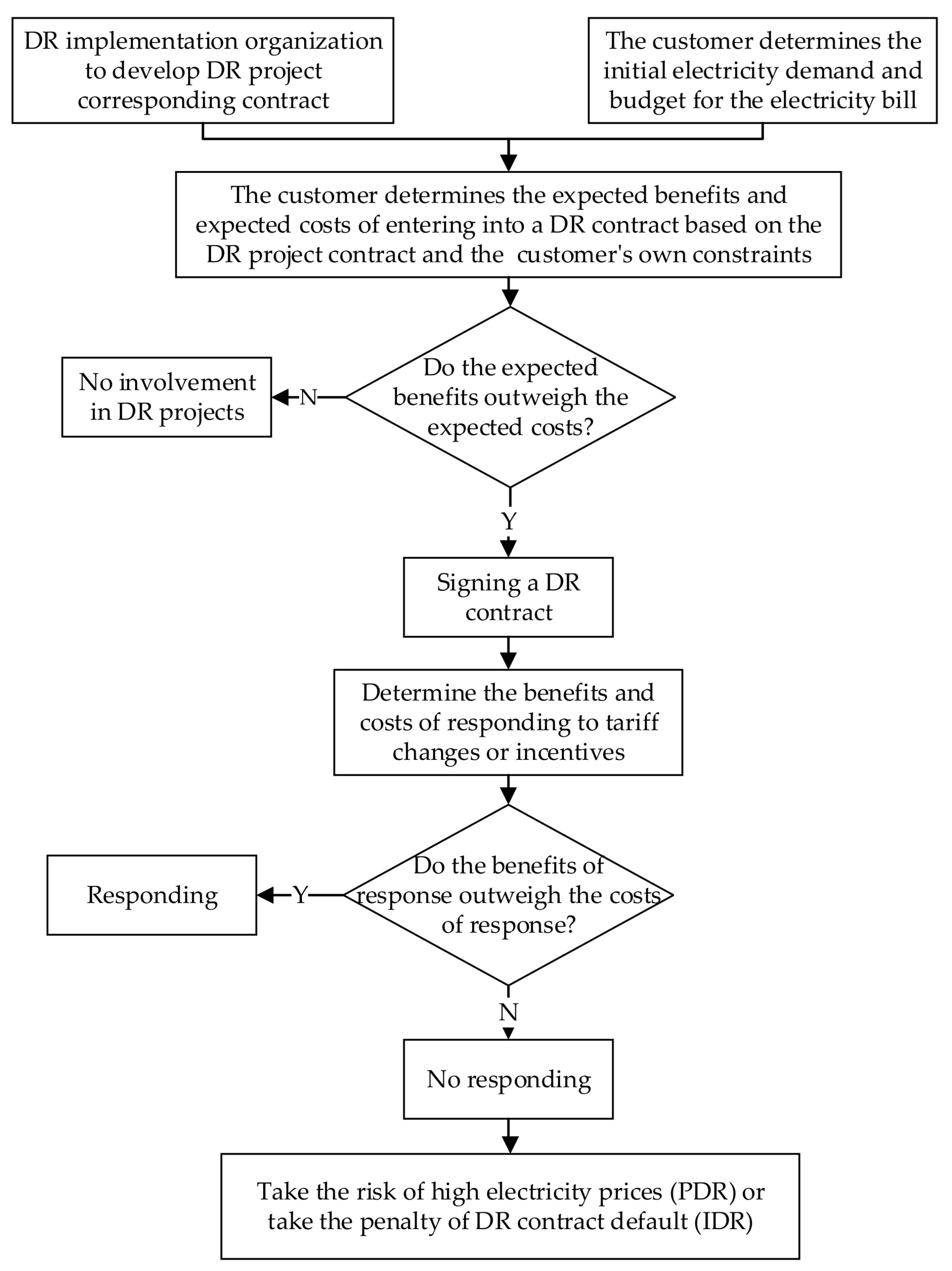
Customers participating in the DR program need to meet the precondition that their rational power usage arrangement has a positive impact on the economy and stability of power production. The advantages of the DR project can be fully reflected in the collaborative activities between customers and system dispatch agencies to achieve a win–win situation. A dynamic decision-making process for customers to choose to participate in the DR project is shown in Figure 1.

Figure 1.
Typical responding process of DR projects.
As can be seen in Figure 1, the actual decision-making process contains two steps: signing a DR contract and responding during a specific period. Both choices in the above steps are made based on the customer’s cost and benefit analysis.
2.1. Multi-Response Characteristics of DR Resources
DR can generally be classified into two types: incentive-based DR (IDR) and price-based DR (PDR) [2]. Here, for IDR, we consider interruptible load (IL), direct load control (DLC) and transferable load (TL).
As the system has a problem of supply–demand balance due to insufficient idle capacity, excessive peak load, transmission line fault or clean energy forecast deviation, the IL and DLC involved in system regulation adjust their own load according to the contract with the power company. The response costs of IL and DLC can be expressed as follows:
where and Q are the total scheduling cost and response amount of DR resources, respectively. represents the type of load resources involved in the dispatch process. and are the duration of response and the interval hours between two adjacent response, and is the maximum responding number.
The weight values in the day-ahead costing are different because of different IDR resources. They are integrated in Equation (2):
where is the dispatch cost of the DR resource at time t. represents the cost weight factor of the DR resource based on the response characteristics. represents the response amount of DR at time t. is the response state variable regarding DR resources’ behavior. represents that DR participates. represents that DR quits.
The response cost of TL in this paper is defined as: when the system has a large peak-to-valley deviation and the load in the peak time is too heavy, it is necessary to reduce the unit startup and shutdown and peak regulation. TL can shift the load response from peak time to valley time based on the dispatch signal. The response cost of TL can be expressed as:
where and are the response cost and the amount of TL at time , respectively. represents the price of the dispatcher’s compensation for the response amount of TL at time t. represents the state variable indicating whether the jth TL participates in the responding process.
For PDR in this paper, the cost is expressed as:
where represents the response amount of the PDR resource at time t, represents the day-ahead forecast load. is the locational marginal price (LMP) at time . and are the upper and lower limits of the LMP, respectively. and are the upper and lower limits of the response amount, respectively.
As the LMP is out of the boundary, the PDR resource can choose whether to respond or adjust to the specified load level. The PDR can obtain the corresponding compensation from the power company. The response cost can be expressed as:
where and are the response cost and the volume of PDR at time , respectively. represents the price of the dispatcher’s compensation for the response amount of PDR at time t. represents the state variable indicating whether PDR zth participates in the responding process.
2.2. DR Resource Scheduling Decision Model
As DR resources are involved in system regulation, the dispatch agency tends to integrate all DR resources as virtual output and make them cooperate with thermal units [22]. Similar to the constraints associated with thermal units, there are also relative constraints for DR resources with multiple response characteristics, including response duration constraint, response interval time constraint and response capacity constraint. The comparison of regulation constraints between thermal units and DR resources is listed in Table 2.
Table 2.
Comparison of regulation constraints between thermal units and DR resources.
Constraints of DR resources are modeled as follows.
(1) Maximum response duration constraint
where represents the maximum response hours.
(2) Maximum responding number constraint
where represents the maximum hours in a dispatch cycle
(3) Minimum response interval time constraint
DR resources must have a certain interval time from the last time to receive the scheduling instruction due to their load characteristics. It can be expressed as:
where represents the accumulated interval of the mth DR resource from the last response, and represents the minimum response interval of the mth DR resource.
(4) Load response amount constraint
where and represents the maximum and minimum response amount of mth DR, respectively.
3. DR Resource Allocation Strategy Based on Multiple Response Modes
3.1. Scenario Generation and Reduction Models Considering Wind Uncertainty
The uncertainty of wind speed causes wind power forecast errors, affecting the stable operation of power systems. Wind power forecast errors result from multiple factors such as season, climate, geography, and the distribution of wind farms. If the wind power forecast value is used as the only reference data for day-ahead dispatching, it will inevitably make the dispatch results deviate from the real value.
Therefore, it is necessary to use probabilistic analysis of wind power forecast errors to improve the accuracy of the wind power forecast so that it can be combined with DR to achieve cooperative effects [23]. Wind power forecast errors are generally considered to obey the Gaussian distribution. They are assumed to be with the variance of and a mean value of 0 at time t before the day [24], which can be expressed as:
where and are the predicted value and the actual output of wind power in each period, respectively. represents the standard deviation, set to 0.1 here. represents the wind power forecast error.
(1) Initial scenario generation
To address the uncertainty of the wind power forecast, the Monte Carlo simulation (MCS) method is used to generate the initial scenarios [25]. Here, we set the predicted wind power output at each time of the day as .
A scenario s is a complete scheduling time cycle. The different scenarios form a set of scenarios [26], .
(2) Scenario reduction
The above set of scenarios tends to enlarge the set scale because of the need to ensure the sampling accuracy, which leads to a low efficiency of problem solving. To balance the computation efficiency and accuracy, the backward reduction (BR) method is applied to the scenario reduction process [27].
The probability distance of the set of predicted scenarios for wind farms for two different scenarios is defined as: if scenario and scenario occur with probability and , respectively, and the sum of the probability of all the scenarios is 1, then the probability distance between scenario and scenario can be expressed as:
The process of the set of the wind power forecast scenario includes the following three steps:
- Step 1: Set a set of scenarios as the initial set and make as an empty set. Set the initial iteration number = 0.
- Step 2: Calculate . Each iteration needs to determine the deleted scenario, for example, the kth iteration needs to delete the scenario . Calculate the probability distance between the reserved scenario and , and obtain the scenario with the smallest probability distance , so that its probability is as follows:
- Step 3: Repeat Step 2 until the scenarios with the smallest distance from the deleted scenario set have been found and add them to achieve the goal that the expected number of deleted scenarios is the same as the number of deleted scenarios.
3.2. DR Resource Allocation Model Based on Multiple Response Modes
Considering the multiple response characteristics of DR resources, a day-head dispatch model of power systems is established. Here, we consider the startup/shutdown schedule of thermal units. Thus, the dispatch model in this paper is a mixed-integer nonlinear programming (MINLP) model to reduce the computational complexity of the proposed optimization with optimality guaranteed [28].
(1) Objective function
After DR resources are involved in the dispatch process, the system combining thermal unit and wind power is optimized for the dispatch operation considering the uncertainty of wind power output. The objective function is to minimize the comprehensive expected system cost, which includes the startup and shutdown costs of thermal units. It can be established as:
where is the total cost. , and are the thermal unit operation cost, DR dispatch cost and wind curtailment penalty cost, respectively.
(i) Thermal unit operation cost
Usually, the shutdown cost of thermal units is set as a smaller constant independent of the continuous operation period, while the startup cost is set as an exponential function of the time constant for the already shutdown time. Here, the startup and shutdown costs of the units are simplified as fixed parameters.
where and represent the startup and shutdown status of the ith unit, respectively. and are the fixed startup and shutdown costs of the ith unit, respectively. and represent the startup and shutdown costs of the ith unit, respectively.
The coal cost of a unit is usually a binomial of its output, expressed as:
where , and are the coal cost factors of the ith unit.
To improve the computational efficiency, we use the piecewise linear function to linearize Equation (16) [29].
Then, the thermal unit operation cost can be expressed as:
where represents the number of thermal units, represents a dispatch cycle, and represent the operating state variable and the output of the ith thermal unit at time t.
(ii) Multiple DR resource dispatch cost
The multiple DR resource dispatch cost can be expressed as:
where , and represent the number of IL, TL and PDR resources, respectively.
(iii) Wind curtailment penalty cost
The wind curtailment penalty cost can be expressed as:
where represents the price of the wind curtailment penalty.
(2) Constraint conditions
The constraints regarding this model include individual constraints and system constraints. The individual constraints contain DR resource multivariate response feature constraints and conventional thermal power characteristic constraints. System constraints contain system reserve constraints, power balance constraints and security constraints.
(i) System constraints
- The spinning reserve constraint:
- System network security constraint
We use the DC current model to characterize the system security constraint in the day-ahead scheduling model to ensure the convergence of the solution and computational efficiency. To reduce the solution complexity, only the maximum transmission capacity constraint of the line is considered as:
where represents the active power of the lth branch. and represent the conductance matrix and voltage phase angle, respectively.
- Power balance constraint
- Stability constraint
As the scale of wind power integrated into the system increases, the stability of the system decreases. Thus, the stability of the system requires that the output provided by the thermal units cannot be lower than the minimum level, expressed as:
where is the minimum demand factor to meet the system stability requirements.
(ii) Individual constraints
- The upper and lower limits of the output constraint
- The minimum startup/shutdown time constraint
- The ramping constraint
- The maximum startup and shutdown power constraint
- Constraints of DR resources in Equations (6)–(9).
4. Example Analysis
The verification study was performed in a modified IEEE 30-bus test system. This system, which is shown in Figure 2, has six thermal units, three DRs and one wind farm. Assume that the three DRs, DR1, DR2 and DR3, are located at Buses 5, 7 and 21, respectively. DR1 contains three IDRs, DR2 contains two IDRs and one TL and DR3 contains one PDR. Additionally, the wind farm with a total capacity of 45 MW is located at Bus 28. The simulation time horizon is set to 24 h with intervals of 1 h.
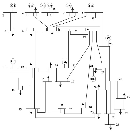
Figure 2.
Topology of the modified 30-bus test system.
To demonstrate the impact of different scenarios on the system dispatch strategy, we design three cases as follows:
- The basic system dispatch without any DR participation.
- Impact of DR (with multiple response modes) on system dispatch.
- Impact of DR on system dispatch cost and wind power consumption.
Case 1:
In this case, no DR resources are involved in system scheduling. Parameters related to the system topology, thermal units and load forecast were obtained from Refs. [30,31], which are shown in Table A1 and Table A2.
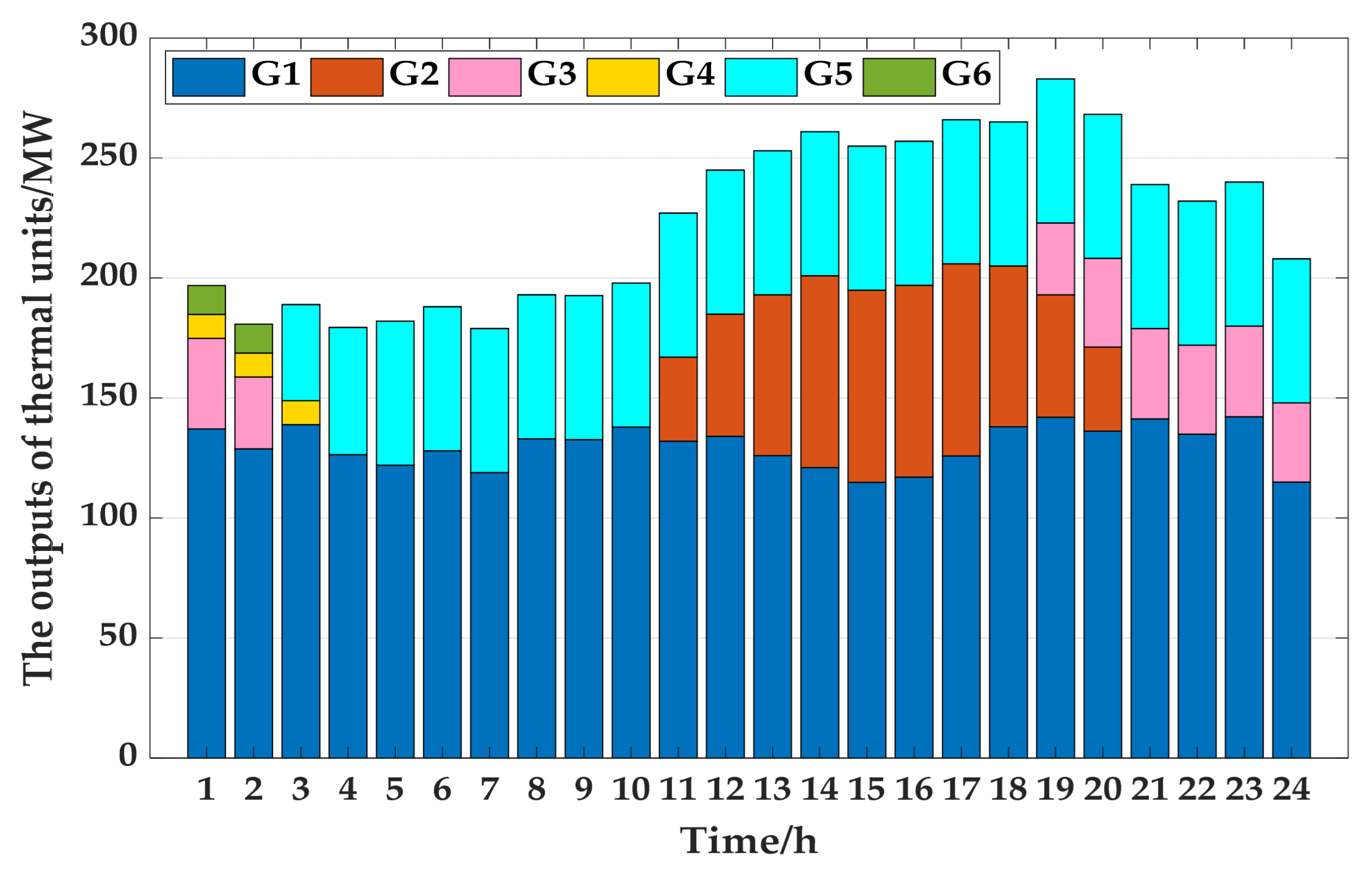
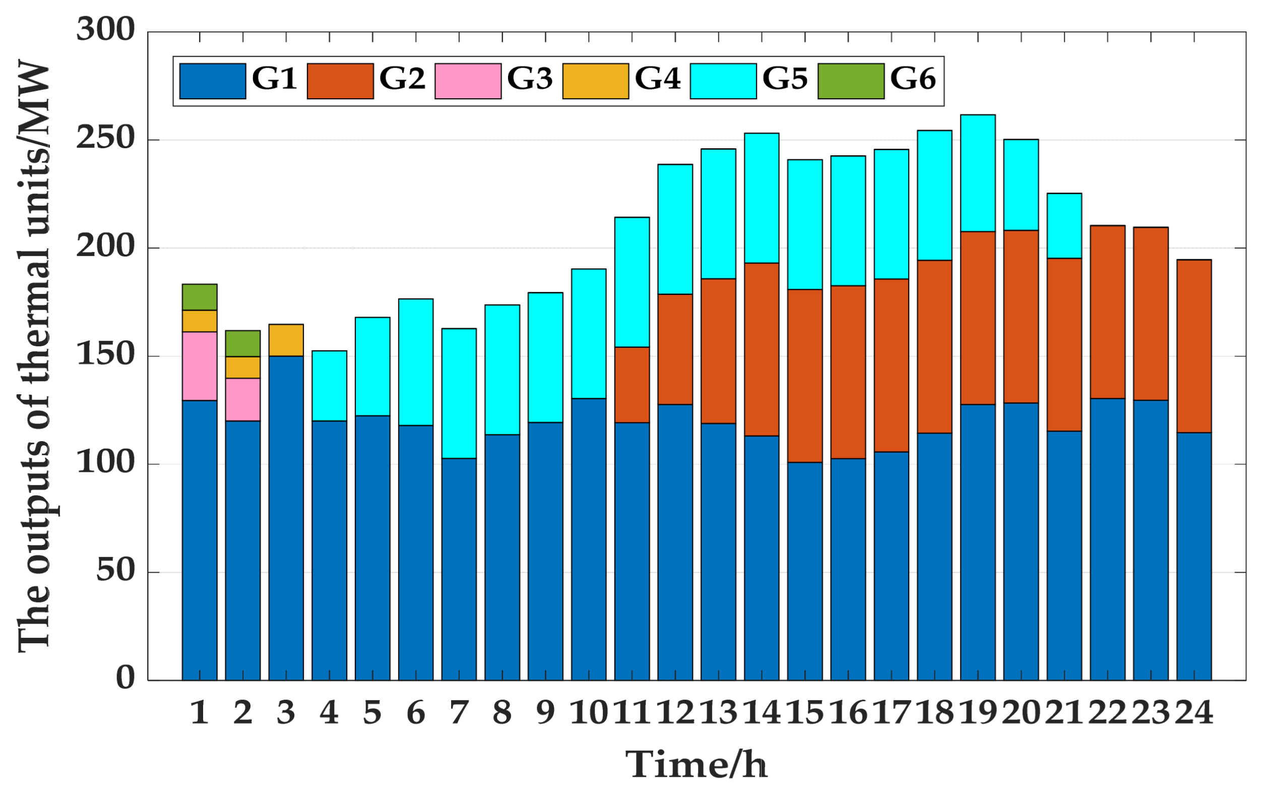
The outputs of six thermal units are optimized based on the scheduling model established in Section 3.2, as shown in Figure 3. The six thermal units are represented as G1–G6. Here, the height of each color block represents the output of each generator at each period. The total cost of system operation is USD 96,808.25, of which the unit operating, startup and shutdown costs are USD 96,171.25 and USD 637, respectively. Additionally, the unit startup/shutdown status can be found in Table 3.
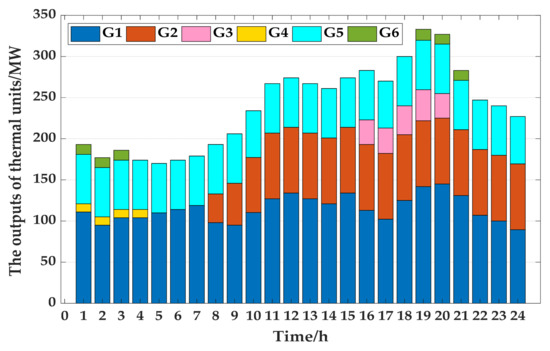
Figure 3.
Outputs of thermal units at each period.
Table 3.
Unit startup/shutdown status within the simulation period.
Case 2:
In this case, DR resources participate in system dispatch. The characteristic parameters of IDR, transferable load and PDR resources are listed in Table A3, Table A4 and Table A5, respectively. The LMP curves of PJM buses and the baseline load curves of PDR resources are given in Figure A1 and Figure A2 (Appendix A).
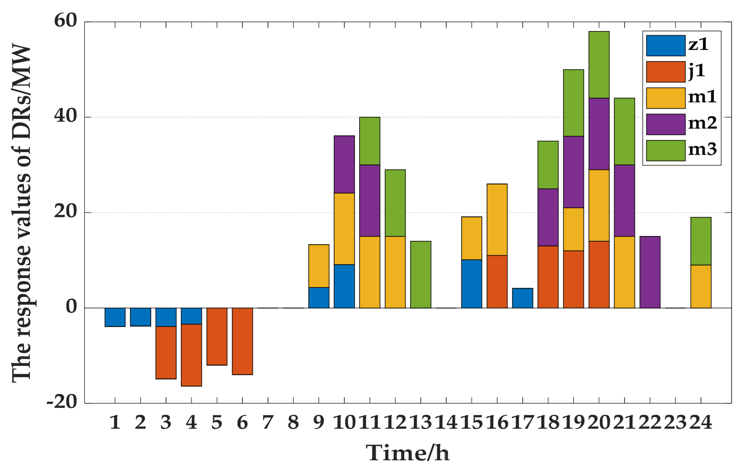
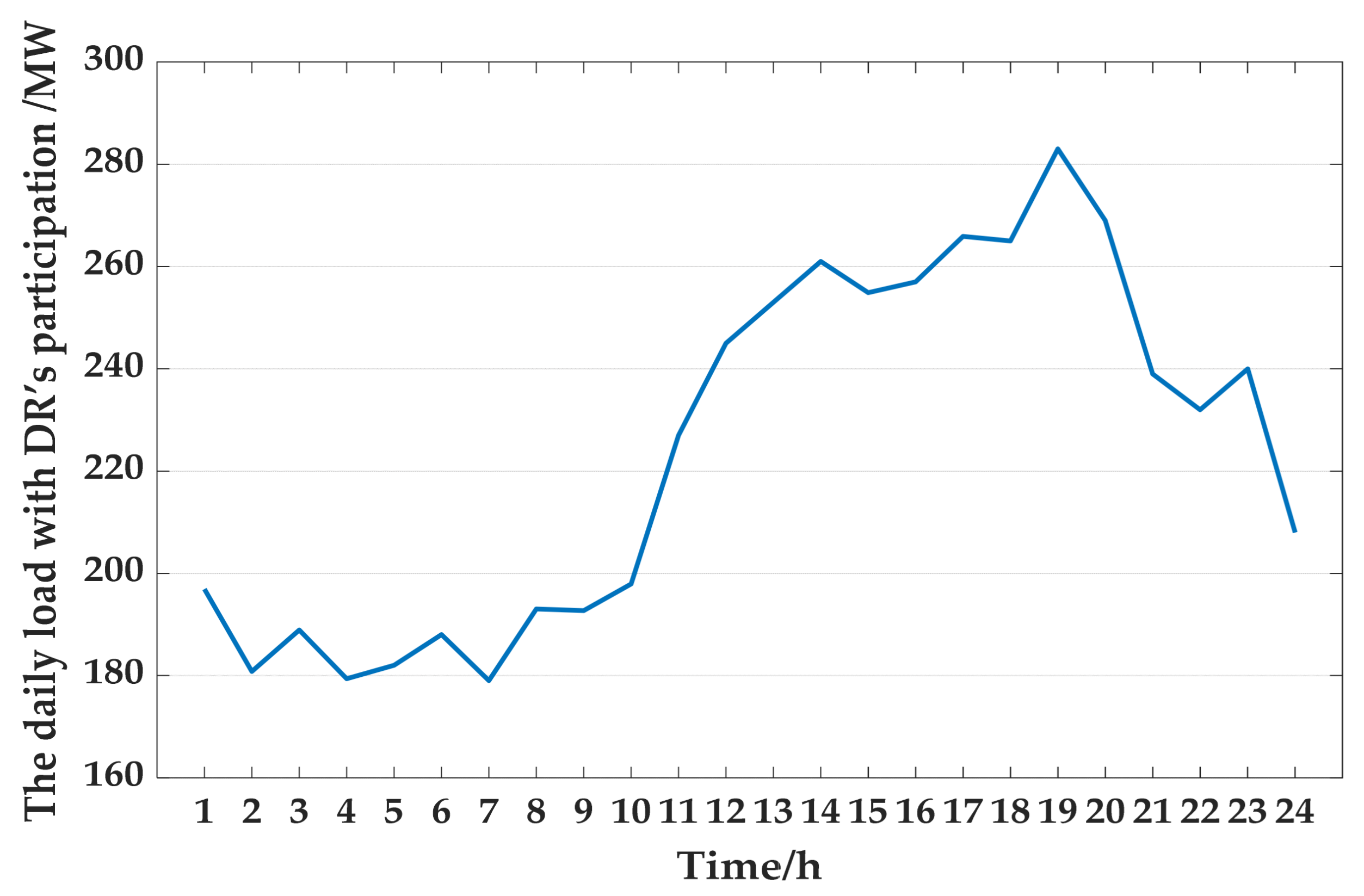
The response values of DRs are shown in Figure 4. The five DRs are represented as z1, j1, m1, m2 and m3. Additionally, z1 and j1 represent the PDR and TL resources, respectively, and m1–m3 are the IDR resources. Here, the height of each color block represents the response value of each DR at each period. The values above/below zero represent that the DR has a positive/negative response. Taking j1 as an example, it reflects that the TL has a negative response from 3:00 to 7:00 and positive responses from 16:00 to 17:00 and 18:00 to 21:00. The thermal unit outputs at each period with DR participation are shown in Figure 5. Additionally, the daily load with DR participation at each period and the unit startup and shutdown status are listed in Figure 6 and Table 4, respectively.

Figure 4.
Response values of DRs at each period in Case 2.
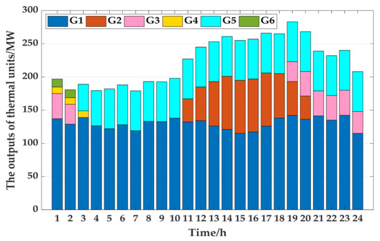
Figure 5.
Outputs of thermal units at each period with DR participation in Case 2.
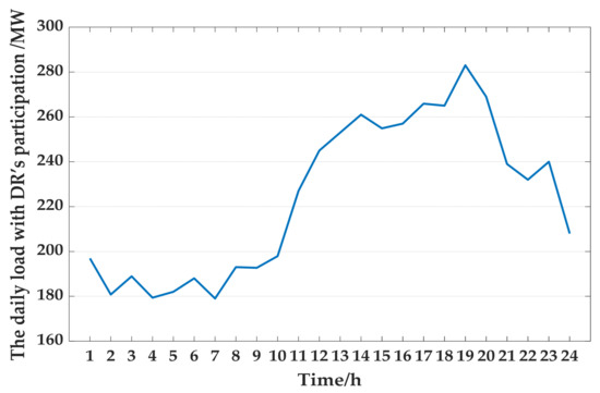
Figure 6.
Daily load with DR participation in Case 2.
Table 4.
The unit start/stop status within the simulation period with DR participation.
The total cost of system operation is USD 93,987.2, of which the unit operating, startup and shutdown costs are USD 90,248.2 and USD 536. The DR cost is USD 3202.
Compared with Case 1, although the participation cost of DR increases to USD 3203, the total cost decreases from USD 96,808.25 to USD 93,987.20 (2.91% lower). The main reason is that the participation of DR reduces the pressure on the peak load regulation of thermal units and makes their startup and shutdown operation more infrequent.
Case 3:
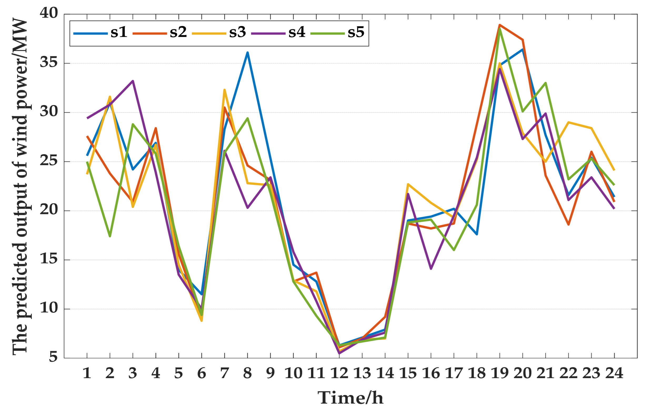
To verify the impacts of DR on wind power consumption, we consider the uncertainties of wind power based on the previous case. After the scenario reduction process, the probabilities of each wind power output scenario can be obtained, as shown in Table 5. The forecast curves of each scenario can be found in Figure 7, which describes the predicted output of wind power in each scenario.
Table 5.
Probability of each uncertain wind power scenario.

Figure 7.
Predicted output of wind power under each scenario.
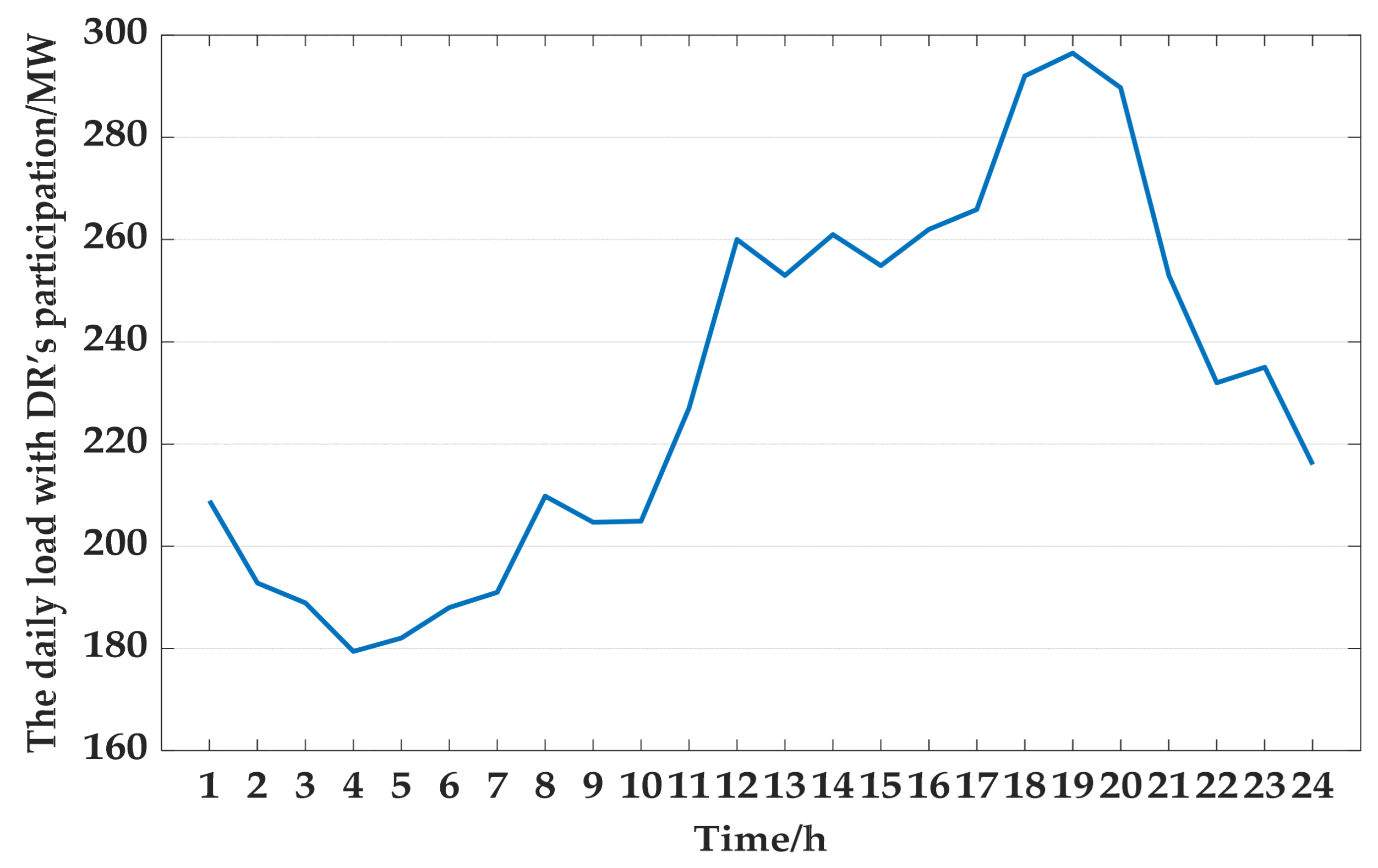
We set = 0.9 and the unit price of wind curtailment penalty as 100 USD/MW. The responding values of DRs and the thermal unit output are listed in Figure 8 and Figure 9, respectively. Furthermore, the daily load with DR participation and the amount of wind curtailment can be found in Figure 10 and Figure 11, respectively. Additionally, to analyze the impacts of DR participation on the total system operation cost, the comparison between the two subcases is listed in Table 6.
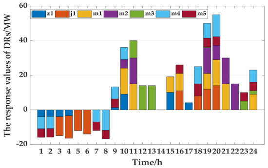
Figure 8.
Response values of DRs at each period in Case 3.

Figure 9.
Outputs of thermal units at each period with DR participation in Case 3.
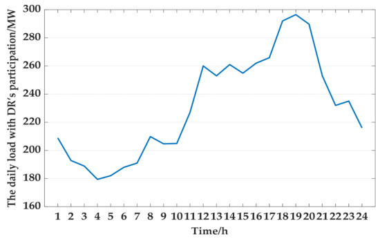
Figure 10.
The daily load with DR participation in Case 3.
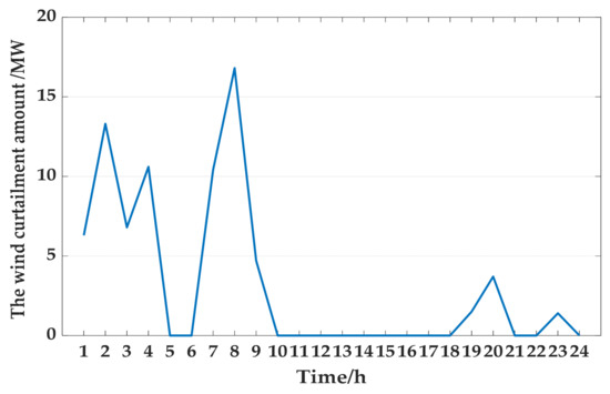
Figure 11.
The wind curtailment amount without DR participation in Case 3.
Table 6.
The impacts of DR participation on system dispatch cost (USD).
As shown in Figure 7 and Table 6, the participation of DRs in the system scheduling reduces both the thermal unit operation cost and wind curtailment penalty cost. In particular, DR participation eliminated additional wind curtailment penalty costs, resulting in a USD 6710 reduction in total cost, which shows that the flexible dispatch strategy and responsiveness of DR resources play an important role in wind power consumption and power balancing.
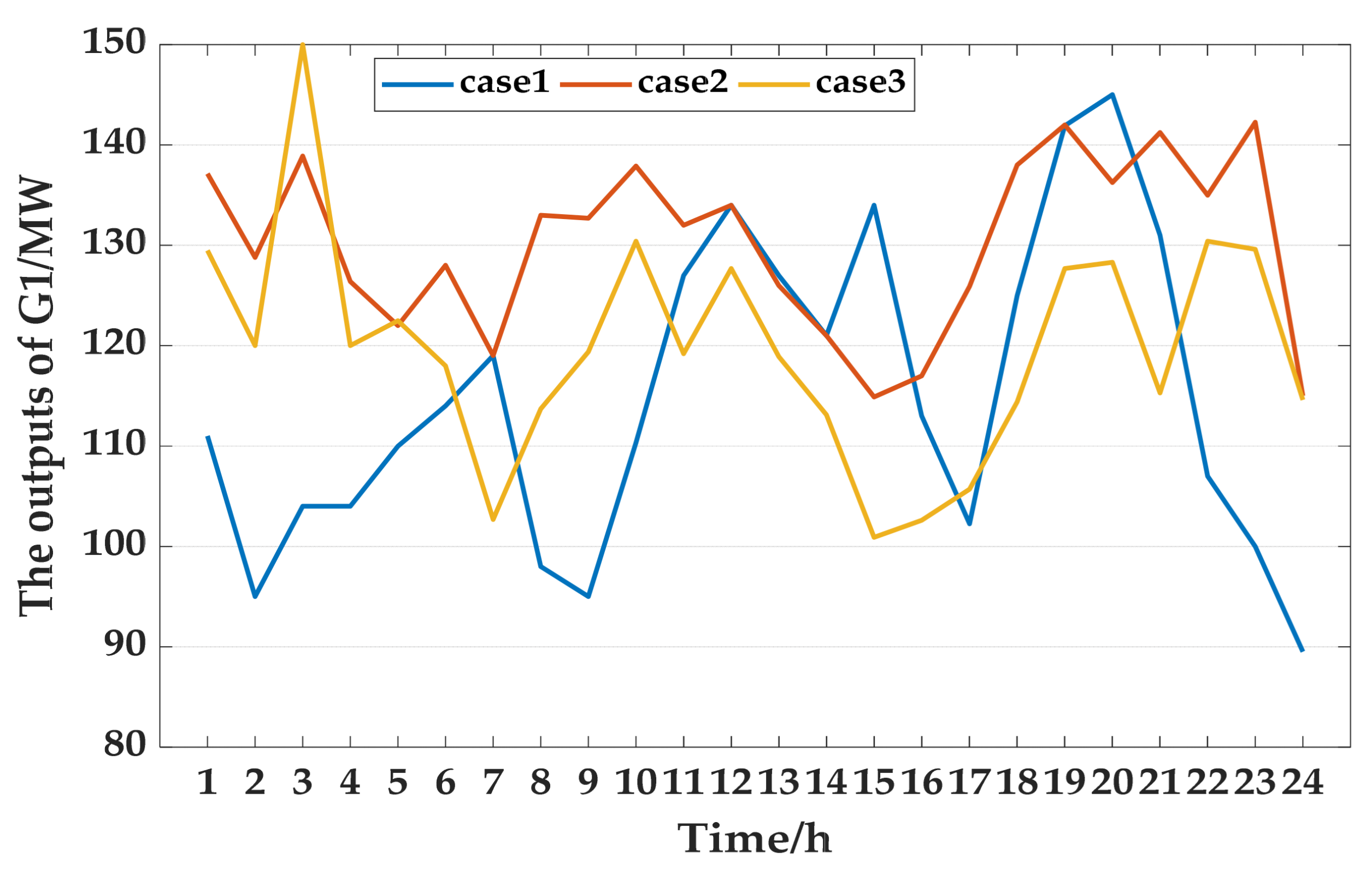
The optimized outputs of thermal units significantly vary in the aforementioned three cases. Taking unit G1 as an example, Figure 12 shows the comparison of the output curves of G1 in the three cases. With the DR resource participating in system dispatch, the fluctuation of the G1 output is clearly smoothed. Additionally, the trend of the G1 output curve in the case where the wind farm is connected to the grid is similar to the case where the wind farm is not connected to the grid. In addition, the overall output of G1 is lower than the former due to wind power consumption.
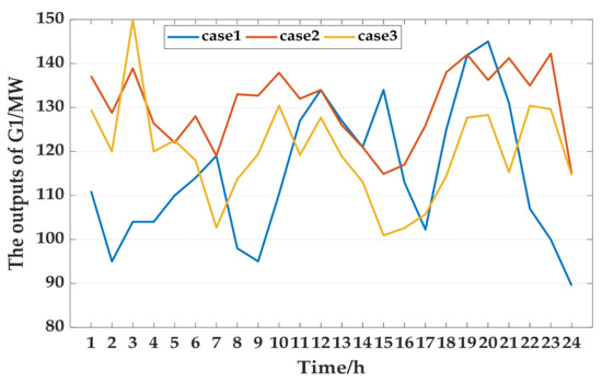
Figure 12.
Outputs of G1 in three cases.
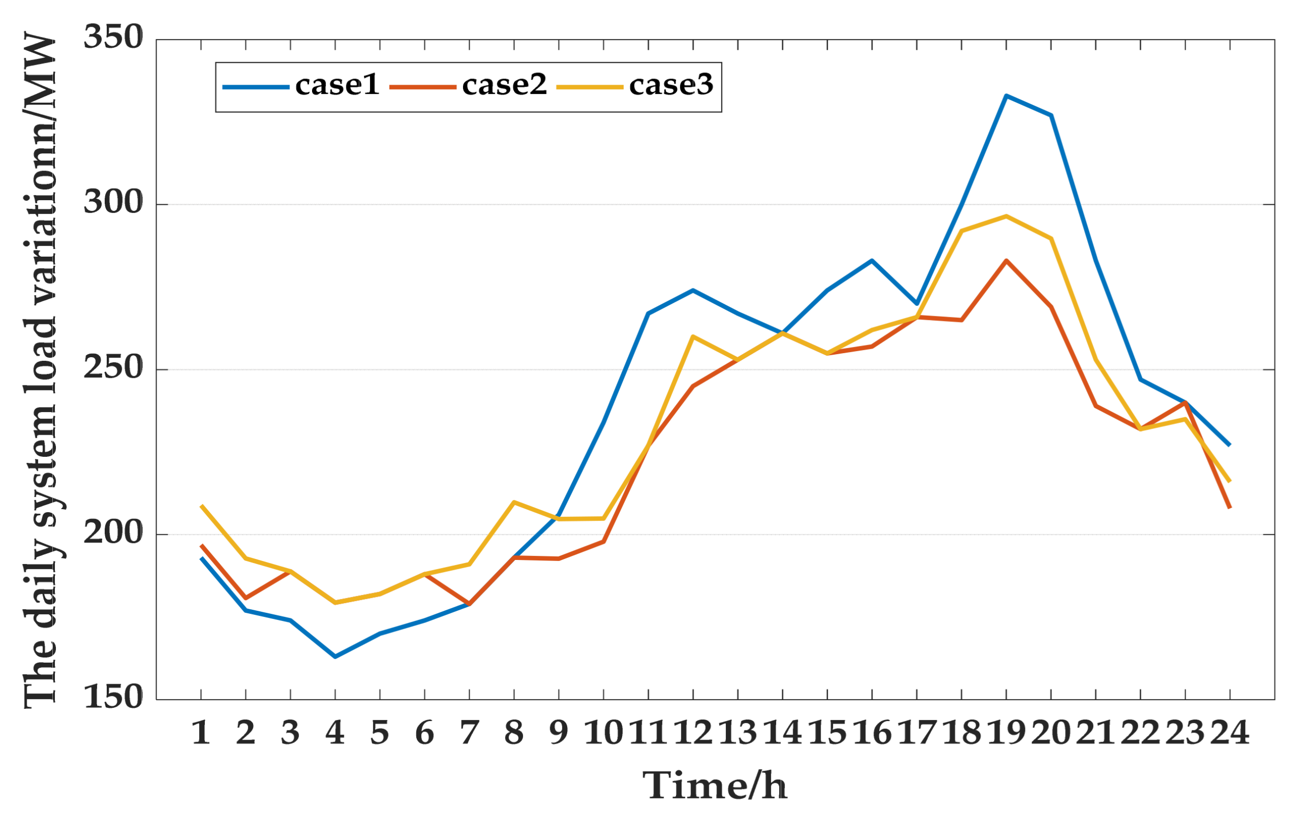
As can be found in Figure 13, the overall level of load decreases, and the curve flattens out after the DR resources participate in system dispatch. DR resources increase the load during the nighttime low-load period while decreasing the load during the daytime peak load period. Thus, the peak-to-valley difference of the system decreases. It can be seen that it plays an important role in relieving the pressure of peak load regulation of thermal units. After the wind power is integrated into the grid, DR resources can reduce the wind power curtailment caused by the anti-peak regulation characteristic. By orderly calling DR resources in 24 h, the sensitivity of its regulation can be used to increase more load to absorb wind power in the valley and reduce load to balance the peaking pressure of thermal power in peak hours.
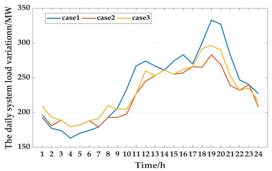
Figure 13.
Variation in daily system load curve.
In Figure 14, represents the total cost, and , and are the costs of thermal units, startup and shutdown and DR, respectively.
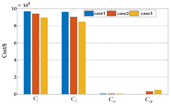
Figure 14.
Comparison of the system operating costs in three cases.
As shown in Figure 11, the costs of unit operating and startup/shutdown on the source side of the system were reduced because of the participation of DR and wind power. Compared to the case without DR participation, although DRs bring extra cost, the total cost is still reduced by 2.91% and 7.64% in Case 2 and Case 3, respectively, because of the greater reduction in the cost of thermal units. Overall, the total cost reduction is due to three main reasons as follows:
- The flexible dispatch of DR resources reduces the cost due to the frequent startup and shutdown costs of thermal units.
- The reduction in peak load decreases the pressure on peak load regulation of thermal units.
- The improved wind power consumption level and the participation of DR resources reduce the high cost of wind curtailment penalty.
5. Conclusions
In this paper, a flexible demand response dispatch strategy considering multiple response modes and wind power uncertainty is presented. First, a DR resource operation decision model based on multiple response characterization of DR resources is formulated. Second, the flexible demand response dispatch strategy is proposed by combining wind power scenario generation and the reduction method. Finally, the effectiveness of the proposed strategy is verified with simulation results.
From the work presented in this paper, general conclusions can be drawn as follows:
- Multiple DR integration has a notable impact on power system dispatch. Meanwhile, when coordinated with thermal units, DR effectively improves the function of peak shaving and valley filling;
- This flexible DR dispatch strategy provides a quantitative assessment of DR integration impacts on system operation cost and wind power consumption;
- It can be applied in day-ahead power system dispatch to help operators effectively evaluate the system state and design demand response mechanisms.
In the future, the energy storage and carbon emission index will be included in our model. Additionally, we plan to combine the load forecast uncertainty and numerical weather prediction model with our framework and make the proposed dispatch strategy more appropriate for real-world scenarios.
Author Contributions
Conceptualization, H.H. and C.W.; Literature review, Y.Z. and T.W.; methodology, H.H., Y.Z. and T.W.; writing—original draft, H.H., Y.Z. and T.W.; writing—review & editing, H.Z., G.S. and Z.W. All authors have read and agreed to the published version of the manuscript.
Funding
This research was funded in part by Fundamental Research Funds for the Central Universities under Grant B200201016 and in part by the Postdoctoral Research Funding Program of Jiangsu Province under Grant 2021K622C.
Institutional Review Board Statement
Not applicable.
Informed Consent Statement
Not applicable.
Data Availability Statement
Some or all data, models, or code that support the findings of this study are available from the corresponding author upon reasonable request.
Conflicts of Interest
The authors declare no conflict of interest.
Appendix A
Table A1.
Line parameters.
Table A1.
Line parameters.
| Line ID | Line Impedance/Ω | Line Capacity/MW | Line ID | Line Impedance/Ω | Line Capacity/MW |
|---|---|---|---|---|---|
| 1–2 | 0.06 | 130 | 16–17 | 0.19 | 16 |
| 1–3 | 0.19 | 130 | 15–18 | 0.22 | 16 |
| 2–4 | 0.17 | 65 | 18–19 | 0.13 | 16 |
| 3–4 | 0.04 | 130 | 19–20 | 0.07 | 32 |
| 2–5 | 0.20 | 130 | 10–20 | 0.21 | 32 |
| 2–6 | 0.18 | 65 | 10–17 | 0.08 | 32 |
| 4–6 | 0.04 | 90 | 10–21 | 0.07 | 32 |
| 5–7 | 0.12 | 70 | 10–22 | 0.15 | 32 |
| 6–7 | 0.08 | 130 | 21–22 | 0.02 | 32 |
| 6–8 | 0.04 | 32 | 15–23 | 0.10 | 16 |
| 6–9 | 0.21 | 65 | 22–24 | 0.18 | 16 |
| 6–10 | 0.56 | 32 | 23–24 | 0.27 | 16 |
| 9–11 | 0.21 | 65 | 24–25 | 0.33 | 16 |
| 9–10 | 0.11 | 65 | 25–26 | 0.38 | 16 |
| 4–12 | 0.26 | 65 | 25–27 | 0.11 | 16 |
| 12–13 | 0.14 | 65 | 28–27 | 0.40 | 65 |
| 12–14 | 0.26 | 32 | 27–29 | 0.42 | 16 |
| 12–15 | 0.13 | 32 | 27–30 | 0.60 | 16 |
| 12–16 | 0.20 | 32 | 29–30 | 0.45 | 16 |
| 14–15 | 0.20 | 16 | 8–28 | 0.20 | 32 |
| - | - | - | 6–28 | 0.06 | 32 |
Table A2.
Thermal power unit parameters.
Table A2.
Thermal power unit parameters.
| Unit ID | Location Bus | Unit Operating Parameters | Maximum Output/MW | Minimum Output/MW | Initial Status | ||
|---|---|---|---|---|---|---|---|
| a | b | c | |||||
| 1 | 1 | 0.001 | 15.7 | 116.3 | 150 | 50 | 1 |
| 2 | 2 | 0.002 | 15.3 | 89 | 80 | 20 | 0 |
| 3 | 5 | 0.005 | 15.6 | 54 | 50 | 15 | 1 |
| 4 | 8 | 0.001 | 19.4 | 82 | 100 | 10 | 1 |
| 5 | 11 | 0.005 | 15.3 | 45.2 | 60 | 10 | 0 |
| 6 | 13 | 0.006 | 20.3 | 39.3 | 40 | 12 | 1 |
| Unit | Location Node | Minimum Downtime | Minimum Startup Time | Upward Ramping Rate | Downward Ramping Rate | Maximum Starting Power | Maximum Stopping Power |
| 1 | 1 | 3 | 2 | 30 | 30 | 80 | 70 |
| 2 | 2 | 0 | 0 | 16 | 16 | 35 | 35 |
| 3 | 5 | 3 | 3 | 12 | 12 | 30 | 30 |
| 4 | 8 | 4 | 3 | 20 | 22 | 55 | 45 |
| 5 | 11 | 0 | 0 | 13 | 12 | 40 | 30 |
| 6 | 13 | 3 | 3 | 10 | 10 | 30 | 20 |
Table A3.
IDR characteristic parameter.
Table A3.
IDR characteristic parameter.
| DR Resources Providers | Resource Number | Cost Coefficient | Maximum Response Duration/h | Maximum Response Capacity/MW | Minimum Response Capacity/MW |
|---|---|---|---|---|---|
| m1 | 9 | 6 | 15 | 5 | |
| D1 | m2 | 7 | 4 | 15 | 8 |
| m3 | 8 | 3 | 14 | 7 | |
| D2 | m4 | 11 | 5 | 15 | 7 |
| m5 | 14 | 4 | 10 | 5 | |
| DR Resources Providers | Resource Number | Maximum Response Number of Times | Minimum Response Interval time/h | — | — |
| D1 | m1 | 4 | 2 | — | — |
| m2 | 2 | 3 | — | — | |
| m3 | 3 | 2 | — | — | |
| D2 | m4 | 4 | 2 | — | — |
| m5 | 5 | 2 | — | — |
Table A4.
Transferable load characteristic parameter.
Table A4.
Transferable load characteristic parameter.
| DR Resources Providers | Resource Number | Cost Coefficient | Total Transferable Duration | Maximum Response Capacity | Minimum Response Capacity |
|---|---|---|---|---|---|
| D2 | J1 | 9 | 4 | 15 | 10 |
Table A5.
PDR resource characteristic parameter.
Table A5.
PDR resource characteristic parameter.
| DR Resources Providers | Resource Number | Maximum Load Level/mw | Minimum Load Level/mw | Tariff Response Upper Threshold/USD | Tariff Response Lower Threshold/USD |
|---|---|---|---|---|---|
| D3 | Z1 | 33 | 8 | 38 | 25 |
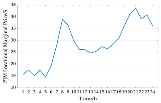
Figure A1.
PJM locational marginal price.
Figure A1.
PJM locational marginal price.
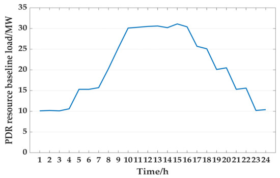
Figure A2.
PDR resource baseline load curve.
Figure A2.
PDR resource baseline load curve.

References
- Jordehi, A.R. Optimisation of demand response in electric power systems, a review. Renew. Sustain. Energy Rev. 2019, 103, 308–319. [Google Scholar] [CrossRef]
- Qdr, Q. Benefits of demand response in electricity markets and recommendations for achieving them. US Dep. Energy Wash. DC USA Tech. Rep. 2006, 2006, 73–75. [Google Scholar]
- Xiang, Y.; Cai, H.; Gu, C.; Shen, X. Cost-benefit analysis of integrated energy system planning considering demand response. Energy 2020, 192, 116632. [Google Scholar] [CrossRef]
- Lynch, M.Á.; Nolan, S.; Devine, M.T.; O’Malley, M. The impacts of demand response participation in capacity markets. Appl. Energy 2019, 250, 444–451. [Google Scholar] [CrossRef] [Green Version]
- Wang, X.; Huang, W.; Tai, N.; Shahidehpour, M.; Li, C. Two-stage full-data processing for microgrid planning with high penetrations of renewable energy sources. IEEE Trans. Sustain. Energy 2021, 12, 2042–2052. [Google Scholar] [CrossRef]
- Aghajani, G.R.; Shayanfar, H.A.; Shayeghi, H. Demand side management in a smart micro-grid in the presence of renewable generation and demand response. Energy 2017, 126, 622–637. [Google Scholar] [CrossRef]
- Ahmadi, S.E.; Rezaei, N. A new isolated renewable based multi microgrid optimal energy management system considering uncertainty and demand response. Int. J. Electr. Power Energy Syst. 2020, 118, 105760. [Google Scholar] [CrossRef]
- Zhao, H.T.; Zhu, Z.C.; Yu, E.K. Research on demand response market and demand response project in power market. Power Syst. Technol. 2010, 34, 146–153. [Google Scholar]
- Sun, Q. Application Research of Price-Based Demand Response Decision Optimization Model; North China University of Electric Power: Beijing, China, 2016. [Google Scholar]
- Lu, Q.; Zhang, Y. Demand response strategy of game between power supply and power consumption under multi-type user mode. Int. J. Electr. Power Energy Syst. 2021, 134, 107348. [Google Scholar] [CrossRef]
- Cui, Y.; Zhang, J.R.; Wang, Z.; Wang, T.; Zhao, Y.T. Day-ahead dispatching strategy for wind-light-thermal co-generation system with price-based demand response. Chin. J. Electr. Eng. 2020, 40, 3103–3114. [Google Scholar]
- Dou, X.; Wang, J.; Wang, Z.; Ding, T.; Wang, S. A decentralized multi-energy resources aggregation strategy based on bi-level interactive transactions of virtual energy plant. Int. J. Electr. Power Energy Syst. 2021, 124, 106356. [Google Scholar] [CrossRef]
- Tuan, L.A.; Bhattacharya, K. Competitive framework for procurement of interruptible load services. IEEE Trans. Power Syst. 2003, 18, 889–897. [Google Scholar] [CrossRef]
- Mohseni, S.; Brent, A.C.; Kelly, S.; Browne, W.N.; Burmester, D. Modelling utility-aggregator-customer interactions in interruptible load programmes using non-cooperative game theory. Int. J. Electr. Power Energy Syst. 2021, 133, 107183. [Google Scholar] [CrossRef]
- Aminifar, F.; Fotuhi-Firuzabad, M.; Shahidehpour, M. Unit commitment with probabilistic spinning reserve and interruptible load considerations. IEEE Trans. Power Syst. 2009, 24, 388–397. [Google Scholar] [CrossRef]
- Mansoori, A.; Fini, A.S.; Moghaddam, M.P. Power System Robust Day-ahead Scheduling with the Presence of Fast-Response Resources Both on Generation and Demand Sides under High Penetration of Wind Generation Units. Int. J. Electr. Power Energy Syst. 2021, 131, 107149. [Google Scholar] [CrossRef]
- Fan, S.; He, G.; Jia, K.; Wang, Z. A novel distributed large-scale demand response scheme in high proportion renewable energy sources integration power systems. Appl. Sci. 2018, 8, 452. [Google Scholar] [CrossRef] [Green Version]
- Jun, D.; Linpeng, N.; Shilin, N.; Peiwen, Y.; Anyuan, F.; Hui, H. A two-stage robust spinning idle capacity optimization model considering demand response and wind power uncertainties. Electr. Power Constr. 2019, 40, 55–64. [Google Scholar]
- Jin, S.; Botterud, A.; Ryan, S.M. Impact of demand response on thermal generation investment with high wind penetration. IEEE Trans. Smart Grid 2013, 4, 2374–2383. [Google Scholar] [CrossRef] [Green Version]
- Cordeiro, M.; Villanueva, D.; Eguía-Oller, P. Optimization of the Electrical Demand of an Existing Building with Storage Management through Machine Learning Techniques. Appl. Sci. 2021, 11, 7991. [Google Scholar] [CrossRef]
- Kong, X.; Quan, S.; Sun, F. Two-Stage Optimal Scheduling of Large-Scale Renewable Energy System Considering the Uncertainty of Generation and Load. Appl. Sci. 2020, 10, 971. [Google Scholar] [CrossRef] [Green Version]
- Niu, W.J.; Li, Y.; Wang, B. Demand response virtual power plant modeling considering uncertainty. Chin. J. Electr. Eng. 2014, 34, 3630–3637. [Google Scholar]
- Klobasa, M. Analysis of demand response and wind integration in Germany’s electricity market. IET Renew. Power Gener. 2010, 4, 55–63. [Google Scholar] [CrossRef]
- Doherty, R.; O’malley, M. A new approach to quantify reserve demand in systems with significant installed wind capacity. IEEE Trans. Power Syst. 2005, 20, 587–595. [Google Scholar] [CrossRef]
- Safdarian, A.; Fotuhi-Firuzabad, M.; Aminifar, F. Compromising wind and solar energies from the power system adequacy viewpoint. IEEE Trans. Power Syst. 2012, 27, 2368–2376. [Google Scholar] [CrossRef]
- Xin, A.; Shupeng, Z.; Qun, Z.R. Research on optimal scheduling model with interruptible load based on scenario analysis. Chin. J. Electr. Eng. 2014, 34, 25–31. [Google Scholar]
- Lei, Y. Research on the Unit Combination Problem of Power Systems Containing Wind Farms Based on Scenario Analysis; Shandong University: Jinan, China, 2013. [Google Scholar]
- Ding, T.; Lin, Y.; Bie, Z.; Chen, C. A resilient microgrid formation strategy for load restoration considering master-slave distributed generators and topology reconfiguration. Appl. Energy 2017, 199, 205–216. [Google Scholar] [CrossRef]
- Arroyo, J.M.; Conejo, A.J. Optimal response of a thermal unit to an electricity spot market. IEEE Trans. Power Syst. 2000, 15, 1098–1104. [Google Scholar] [CrossRef]
- Ademovic, A.; Bisanovic, S.; Hajro, M. A genetic algorithm solution to the unit commitment problem based on real-coded chromosomes and fuzzy optimization. In Proceedings of the Melecon 2010—2010 15th IEEE Mediterranean Electrotechnical Conference, Valletta, Malta, 26–28 April 2010; pp. 1476–1481. [Google Scholar]
- Niknam, T.; Narimani, M.R.; Jabbari, M. Dynamic optimal power flow using hybrid particle swarm optimization and simulated annealing. Int. Trans. Electr. Energy Syst. 2013, 23, 975–1001. [Google Scholar] [CrossRef]


Publisher’s Note: MDPI stays neutral with regard to jurisdictional claims in published maps and institutional affiliations. |
© 2021 by the authors. Licensee MDPI, Basel, Switzerland. This article is an open access article distributed under the terms and conditions of the Creative Commons Attribution (CC BY) license (https://creativecommons.org/licenses/by/4.0/).