Abstract
Lung cancer is a deadly cancer that causes millions of deaths every year around the world. Accurate lung nodule detection and segmentation in computed tomography (CT) images is a vital step for diagnosing lung cancer early. Most existing systems face several challenges, such as the heterogeneity in CT images and variation in nodule size, shape, and location, which limit their accuracy. In an attempt to handle these challenges, this article proposes a fully automated deep learning framework that consists of lung nodule detection and segmentation models. Our proposed system comprises two cascaded stages: (1) nodule detection based on fine-tuned Faster R-CNN to localize the nodules in CT images, and (2) nodule segmentation based on the U-Net architecture with two effective blocks, namely position attention-aware weight excitation (PAWE) and channel attention-aware weight excitation (CAWE), to enhance the ability to discriminate between nodule and non-nodule feature representations. The experimental results demonstrate that the proposed system yields a Dice score of and , and an intersection over union (IoU) of and on the publicly available LUNA16 and LIDC-IDRI datasets, respectively.
1. Introduction
According to the World Health Organization (WHO), lung cancer is the leading cause of cancer deaths in 2020 (1.80 million deaths) [1]. The estimated number of new cases has risen to 2.89 million, and the number of deaths may reach 2.45 million worldwide by 2030 [2]. These deaths could be avoidable by an early diagnosis with a proper treatment plan. The National Lung Screening Trial (NLST) showed that the mortality of lung cancer is reduced by 20% by emphasizing the significance of nodule detection and assessment [3]. Many studies have shown the efficacy of computed tomography (CT) screening for lung cancer diagnosis and the detection of subsolid nodules, as well as suspected/unsuspected lung cancer nodules [4].
CT imaging technology helps make an efficient investigation to discover pulmonary nodules. CT imaging technology generates a hundred images of the lung within a second by a single scan. It is difficult for radiologists to manually detect and segment the lung nodules from such a high number of images. In this context, computer-aided diagnosis (CAD) systems have assisted radiologists in the automated diagnosis of lung cancer and pulmonary diseases over the last several years. The authors of [5] noted that the use of an accurate lung nodule CAD system accelerates the entire diagnosis and radiotherapy process, such that patients can perform the required radiation or photon therapy on the same day. CAD systems mainly depend on the detection and segmentation of various pulmonary parts. Computer-aided detection (CADe) systems identify the region of interest (ROI) in the lung nodule, while computer-aided segmentation (CASe) systems segment the nodule region and determine its boundaries.
Automated analysis of lung CT images is essential to measure the properties of lung nodules for identifying malignancy in a tumor. Lung nodule segmentation systems can determine malignancy by analyzing nodule size, shape, and change rate [6]. Although many automated nodule detection/segmentation systems have been presented in the last years [7,8,9], their accuracies are not high due to several challenges, such as the heterogeneity of CT images and the variation present in nodule size, shape, and location.
In the last years, deep convolutional neural networks (CNNs) have been widely used to handle the lung nodule detection and segmentation problem, achieving promising results [7,8,9,10,11,12,13]. CNNs can learn complex features to detect and segment the nodule accurately. However, existing nodule segmentation systems use deep learning models to segment nodules from the whole-input CT images. This reduces the segmentation precision because the input images are usually resized before feeding into the deep learning model. Such resizing processes yield artifacts that badly affect the objects’ boundaries and details.
In an attempt to handle the challenges that accompany the automated segmentation of lung nodules, in this article, we propose the AWEU-Net method for a lung nodule detection and segmentation system based on deep learning. AWEU-Net is a fully automated deep learning-based framework that includes two cascaded stages. In the first stage, AWEU-Net automatically detects lung nodules based on a fine-tuned Faster R-CNN model. In the second stage, AWEU-Net automatically delineates lung nodules from the ROI which results from the first stage based on a U-Net architecture with two powerful blocks via position attention-aware weight excitation (PAWE) and channel attention-aware weight excitation (CAWE). Both blocks help model the correlation between the spatial and channel features and encourage the CNN to learn the most relevant features that enhance its ability to discriminate between nodule and non-nodule feature representations. The contributions of this article can be listed as follows:
- •
- A fully automated deep learning-based framework called AWEU-Net is proposed for improving the accuracy of lung nodule detection and segmentation;
- •
- PAWE and CWEU mechanisms are proposed to model the correlation between the spatial and channel features and encourage the CNN model to learn the most relevant features that enhance its ability to discriminate between nodule and non-nodule feature representations;
- •
- A comparative study of different nodule detection models and nodule segmentation models is presented using two publicly available datasets, namely LUNA16 and LIDC-IDRI.
Section 2 of this article discusses the existing lung nodule segmentation systems based on classical computer vision and deep learning techniques. Section 3 introduces the proposed system workflow and model architecture. Section 4 presents and discusses experimental results. Finally, Section 5 concludes the article and highlights a future extension of this research.
2. Related Work
In the literature, several lung nodule detection and segmentation systems have been presented based on classical computer vision and deep learning techniques. Table 1 lists some common lung nodule segmentation techniques. Below, we present and discuss classical computer vision-based and deep learning-based lung nodule segmentation methods.

Table 1.
Summary of existing lung nodule segmentation methods. The undeclared information is marked with dashes (-) in the referred literature. Aug., morph, acc and IoU stand for augmentation, morphological, segmentation accuracy and intersection over union, respectively.
2.1. Classical Computer Vision-Based Approaches
In the field of lung nodule analysis, many computer vision methods based on hand-crafted features have been used, such as region growing [14], active contours [15], level sets [16], graph cuts [17], adaptive thresholding [18], Gaussian mixture models (GMM) with fuzzy C-means [19], and region-based fast marching [20]. However, it is difficult to generalize a nodule segmentation model based on hand-crafted features that can be useful for CT images. All the aforementioned traditional approaches are semi-automated or depend on several image pre-processing and post-processing techniques. For instance, a contrast-based region growing method and fuzzy connectivity map of the object of interest (i.e., nodule) were used in [14] to segment various types of pulmonary nodules. This method did not perform adequately with irregular nodules due to merging different criteria in the region growing technique that needed a fine-tuning for parameters of the setting. Geometric active contours with a marker-controlled watershed as well as Markov random field (MRF) was used in [15] to segment the lung nodule. In turn, ref. [16] used a shape prior hypothesis along with level sets that iteratively minimized the energy needed to segment juxtapleural pulmonary nodules. However, these two methods depend on manually selected seeds in the nodule region, and thus the precision of the segmentation process depends on the proper selection of seeds. A graph cut algorithm with an expectation-maximization (EM) algorithm was proposed in [17] for lung segmentation on chest CT images. This algorithm yields acceptable segmentation results; however, it has a high computational cost because it focuses on training a GMM and searching on the corresponding graph using a heuristic searching algorithm. Ref. [18] used an adaptive thresholding technique along with a watershed transform to detect lung nodules. However, this approach mainly relies on different pre-processing and post-processing procedures. Ref. [19] combined GMM knowledge within the conventional fuzzy C-means method to improve the robustness of pulmonary nodule segmentation. The major disadvantage of fuzzy C-means algorithms is that they are sensitive to noise, outliers, and primary cluster selection. A region-based approach was introduced in [20] by using the fast marching method, which gives a precise segmentation of the nodule and can properly handle juxtapleural and juxtavascular nodules. The main disadvantage of region growing segmentation is the fact that the resulting histograms do not provide any spatial knowledge of the input images.
2.2. Deep Learning-Based Approaches
Recently, many researchers have developed various deep learning-based systems for lung nodule detection and segmentation. The authors of [21] introduced a lung CT image segmentation method using the U-net architecture proposed in [22], consisting of encoder and decoder networks. With the LIDC-IDRI dataset, they achieved a Dice score coefficient (DSC) of 0.9502. It is worth noting that the model presented in [21] and our method are based on U-Net; however, each one is designed for solving a different problem: ref. [21] fine-tuned U-Net to segment the whole lung from the CT images, while our method integrates two new blocks (CAWE and PAWE) with U-Net to improve the segmentation accuracy of nodules. Ref. [10] used a simple version of the U-Net model for lung nodule segmentation by utilizing only two convolutional layers in the encoder network and two deconvolutional layers in the decoder network, U-Net. The model used different receptive field sizes to enhance nodule feature extraction. Their model yields a DSC improvement of compared to the original U-Net. Besides, ref. [9] presented a dual-branch residual network (DB-ResNet) that achieved results similar to [10]. The major differences between [9] and [10] are the use of convolutional blocks of ResNet [23] in the encoder networks and slightly modified pooling layers.
In turn, ref. [7] combined two U-Net models (named iW-Net) based on user interactions. Their architecture was designed by expecting nodules of only round shapes. The authors combined the weight map and the feature of the model output as a loss function. The iW-Net model gave a final competition performance metric score of on nodule detection and a DSC score of on nodule segmentation. In addition, ref. [13] presented a multiple resolution residual network (MRRN) that is a modification of the ResNet [23]. The modified MRRN network is used as the backbone of the U-Net model. Ref. [13] achieved a DSC score of . A slightly transformed version of U-Net called U-Det was presented in [8], where many hidden layers were used to filter the residual blocks located within the encoder and decoder. With the LUNA16 testing dataset, they achieved a DSC of that was improved to when U-Det applied the Mish activation function proposed in [24] for smoothing and non-monotonic activation.
Most aforementioned lung nodule segmentation methods use deep learning models that segment nodules from the whole-input CT images. However, this can degrade the segmentation precision. This is because the input images are usually resized before feeding to the deep learning model, which yields too many artifacts and badly affects the objects’ boundaries and details. Consequently, in this work, we attempt to build a cascaded lung nodule detection and segmentation system that can outperform the accuracy of the state-of-the-art. Firstly, fine-tuning the important parameters of the state-of-the-art object detection (i.e., Faster-RCNN) is applied to be more appropriate for lung nodule detection and to have an automated system to localize the nodule in CT images. The output of the object detection model is to enable ROI that involves the nodule region. A segmentation model will then be fed with ROIs to segment the exact potential nodule region and properly determine its boundaries. Thus, improving the U-Net model is then achieved by integrating the position attention module (PAWE) and channel attention module (CAWE) to encode contextual information into spatial and channel features. These modules help our segmentation system to accurately distinguish nodules from non-nodules regions and also help in facilitating the model’s training process, since they encourage the model to learn nodules’ relevant features.
3. Proposed Methodology
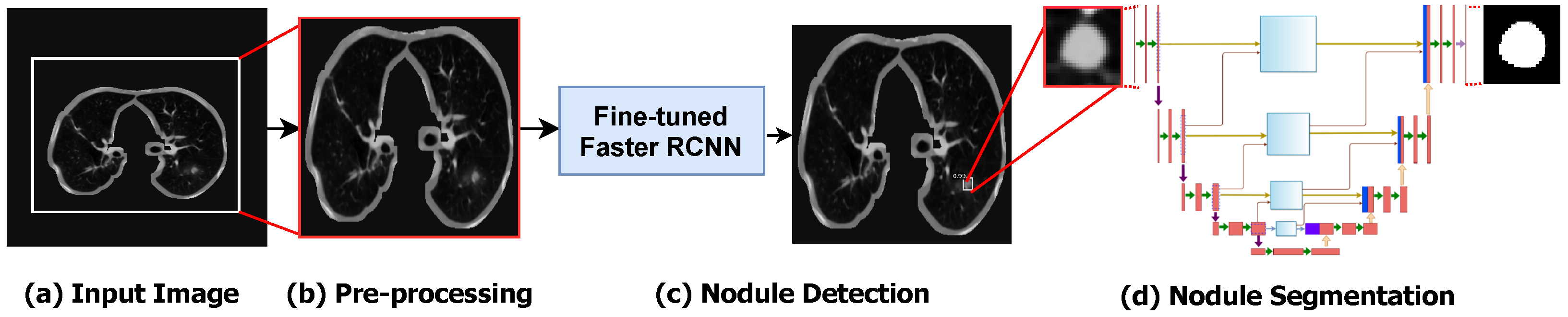
The main components of the proposed framework are shown in Figure 1. As shown, as a pre-processing stage, we represented the 3D CT volumes as 2D CT slices. The Dicom CT slices are transformed into images of “.png” file format. A global thresholding technique is used for separating the lung region from the background in CT images. In order to detect the nodule ROIs from the input CT images, we fine-tuned the Faster R-CNN object detection model to adapt it for lung nodule detection. The detected nodule ROI is then fed to the segmentation model to precisely segment the nodule and its boundaries.

Figure 1.
The step-by-step workflow of the proposed method. (a) The converted input image is extracted from the original CT slice. (b) The pre-processing step for selecting ROI of lung. (c) The detection of lung nodules using Optimized Faster R-CNN. (d) The segmentation of lung nodules using the proposed AWEU-Net model.
3.1. Pre-Processing
The raw CT scans’ data are always available in the Dicom file format. However, to make the images more meaningful and useful for deep learning models, the pylidc [25] library is used for converting the Dicom images to a “.png” file format. Afterwards, a global Otsu binary thresholding technique and morphological dilation are applied on the CT images to separate the lung region from the background, as shown in Figure 1b. Experimentally, we found that the image size of yields the best accuracy with lung nodule detection. Thus, we resized all images to that image size. Finally, we split the dataset into 70% for training, 10% for validation, and 20% for test. For training Faster-RCNN, we convert all ground-truth images to ms-coco format [26], where the dataset is formatted in JSON and is a collection of “info”, “images”, “annotations”, and “categories”.
3.2. Nodule Detection Model
Among all two-stage object detection models, the single-shot detector (SSD) is the fastest detection model, but it is not the most accurate one [27]. In our framework, we aimed at developing an accurate segmentation model; Faster RCNN is considered one of the most accurate detection models in inferring the locations of the target in the input image [28]. Thus, we preferred to choose the Faster RCNN model rather than SSD for localizing the nodules in CT images. In this stage, we attempted to fine-tune the important parameters of the Faster RCNN detection model. We focused on finding the best combination of the learning rate, step size, factor of dropped learning rate , and drop-out ratio to make Faster RCNN more appropriate for lung nodule detection.
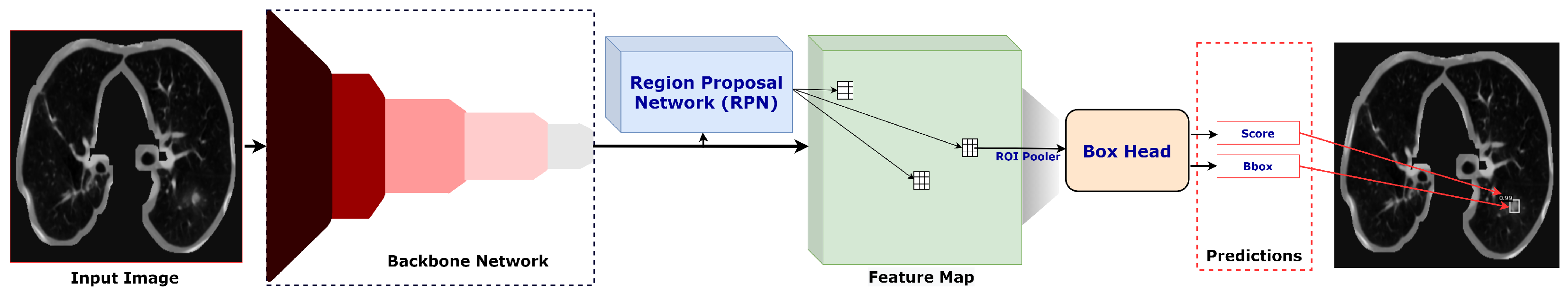
As shown in Figure 2, the Faster-RCNN detection model is a two-stage detection network containing three main blocks: a backbone network, a region proposal network (RPN), and a box head. We used ResNet50 [23] as a backbone network to extract feature maps from the input image. The feature map is then fed into the RPN to perform boundary regression and classification analysis, and the output is a set of ROI candidates. The classification principle is based on whether a candidate ROI is either related to background or to the object (i.e., in our case, tumour nodules). The position and score of the candidate ROI are forwarded to the box head, where the final regression and classification of the object is performed. Finally, the bounding box of the target (nodule) with the classification score is returned from the detection model.
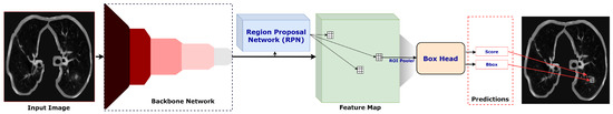
Figure 2.
The detailed architecture of Optimized Faster R-CNN.
3.3. Nodule Segmentation Model
We cropped the ROI based on the bounding box provided by the nodule detection model in the first stage. We resized the ROI to and fed it into the proposed nodule segmentation model. It is obvious that we scaled up the ROI of the nodule, which we did since we believe that is the best way to enhance spatial features, especially for small objects like nodules. By scaling up the input ROIs rather than downsampling them, the deep segmentation network can be better adapted to detect even tiny object boundaries.
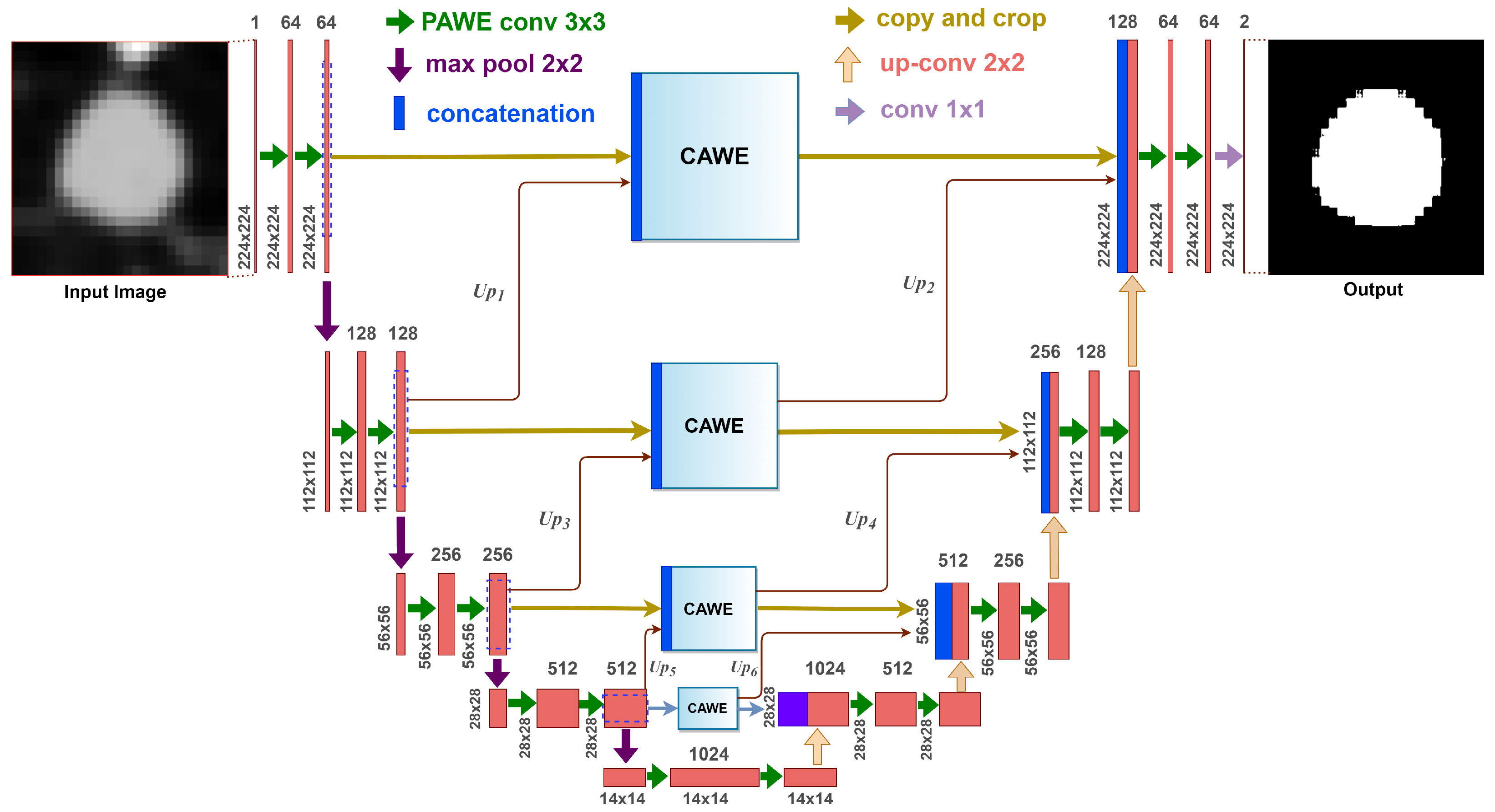
In the second stage of our framework, we propose an attention-aware weight excitation U-Net, AWEU-Net, for our lung nodule segmentation, as shown in Figure 3. This network is based on the U-Net [22], which is a well-known deep learning model for medical image segmentation. The AWEU-Net model learns to segment the input ROIs by determining the boundaries of the nodule region to discriminate between nodules and non-nodule regions. The output of AWEU-Net is a binary image that contains ones for nodule regions and zeros for the others.

Figure 3.
The architecture of the proposed AWEU-Net. The PAWE and CAWE block refers to the position attention-aware weight excitation and channel attention-aware weight excitation, respectively.
The proposed model integrates PAWE and CAWE blocks with U-Net in order to capture the correlation between both spatial and channel features, as well as to enhance the ability to discriminate between nodule and non-nodule feature representations. On the one hand, the feature map resulting from a convolution layer contains a set of channels; each can be a class-specific response comprising high-level features. Since some channels can be correlated, CAWE, which models inter-dependencies among channel maps, is able to highlight inter-dependent feature maps. On the other hand, PAWE helps to capture discriminant feature representations by encoding contextual information into local features extracted by convolution layers. The details about PAWE and CAWE will be discussed in Section 3.4.1 and Section 3.4.2, respectively.
The AWEU-Net architecture is composed of two successive networks: an encoder and a decoder. The encoder consists of four convolution layers. Each encoder layer is composed of a convolution of followed by a PAWE block and a ReLU as an activation function. Four down-sampling blocks with a max pooling of followed by a stride of 2 are used after each encoder layer.
In turn, the decoder consists of four layers, which each also consist of a convolution of followed by a PAWE block, a ReLU and a deconvolution of . In the original UNet, the outputs of the decoder layers (if exiting) were concatenated with the features extracted by the corresponding encoder layers to input to the next decoder layer. In AWEU-Net, we inserted the CAWE blocks between the corresponding layers of the encoder and decoder networks. Each CAWE block is fed with a feature map of the same size as the corresponding encoder layer. The CAWE blocks are fed by the concatenation of the features extracted by the corresponding encoder layer and the upsampling features extracted by the next encoder layers (e.g., Up1, Up3 and Up5 in Figure 3). The output of the CAWE block is fed as an input to the corresponding decoder layer. Additionally, the output feature map of the previous CAWE block is scaled up and also fed to the decoder layer as an input (e.g., Up2, Up4, and Up6 in Figure). In this mechanism, we depend on the features extracted by PAWE and CAWE blocks to enhance the positional and channel low- and high-level features extracted by the encoder network and utilise them for the reconstruction means in the decoder network.
The final output layer of the model applies a convolution of to map the final feature map of 64 channels to the number of targeted segmentation classes (i.e., in our case two classes related to the nodule and the background).
3.4. Attention Mechanism
For semantic segmentation, the scene can involve objects (e.g., cars) which are different in views, scales, and lighting. Thus, the features extracted by CNNs corresponding to the same object could have diversities, since CNN filters yield diverse local receptive fields. These diversities in the pixels corresponding to the same label/object cause intra-class inconsistency and affect the segmentation accuracy [29]. Regarding nodule segmentation, the nodules, in general, have different sizes that can yield features with intra-class inconsistency. Consequently, with our framework, we inserted global contextual attention models in both spatial and channel dimensions in the UNet network to explore relationships between features extracted in different layers of the encoder network before feeding to the decoder to reconstruct the segmented images.
In the next sub-sections, we will present the two attention modules PAWE and CAWE, which help our network to capture contextual information in spatial and channel dimensions, respectively.
3.4.1. Position Attention-Aware Weight Excitation (PAWE)
For accurate nodule semantic segmentation, deep learning models have to capture discriminant features of the nodules and background in a CT image. These features can be captured by aggregating the spatial context information from local features [30]. To model contextual relationships over local features, PAWE is able to enhance the local feature representation through encoding long-range contextual information. The process of PAWE can be elaborated as follows.
The PAWE block consists of two sub-blocks: the position attention block (PAB) and the weight excitation block (WEB). To demonstrate the proposed PAWE block, let the input feature be , where C, H and W are channel, height and width, respectively (see Figure 4). In the PAB block, Y is fed into 3 convolutions of called A, B and C, respectively. The first 2 produced feature maps, are provided by the first 2 convolutions A and B,where p superscript is referred to as ”postion”. and feature maps are then reshaped into . A matrix multiplication is applied to the transposition of and , producing a spatial attention map, , by using a softmax function:
where indicates the ith position’s associated position of jth. The softmax function attempts to learn the relationship between two spatial positions in the input feature maps.
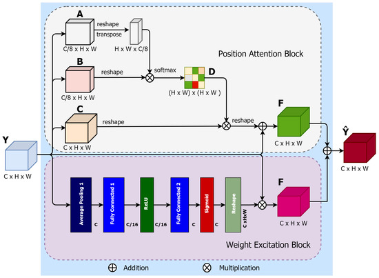
Figure 4.
Illustration of the proposed PAWE block.
In addition, the output of the third convolutional layer is also reshaped to the same shape of the input feature map Y and then multiplied by a permuted order of the spatial attention map of (1). The final output is reshaped to to provide the final feature map of PAB block, F, as
where is defined as 0 as explained in [29]. The resulting feature at each feature position is a weighted sum of all the neighbours of the original features.
In the WEB, a sub-block for location-based weight excitation (LWE) proposed in [31] is used. The LWE provides fine-grained weight-wise attention during back propagation. The WEB shown in (Figure 4) can be defined as:
where is the weights across the jth output channel. The average pooling layer, , averages the values of each . and are two ReLU activation functions. and are two fully connected layers.
The output feature from WEB is reshaped and multiplied to the input feature map. Finally, an element-wise sum operation is performed between the feature maps from the PAB and WEB to produce the final PAWE features, as follows:
This process generates a global contextual description and aggregates the context according to a spatial weighted attention map by creating spatial-relevant weighted features, which provide common weight excitation and enhance the intra-class semantic coherence of the input features maps.
3.4.2. Channel Attention-Aware Weight Excitation (CAWE)
Each class-specific response (in our case, there are two classes of nodules and background) is related to each channel of local features extracted by the encoder layers. Different semantic class responses are correlated with each other [29]. Thus, to improve the feature representation of each class-specific response, the proposed CAWE block can properly highlight the interdependence between channels in feature maps and explicitly model inter-dependencies between channels. The process of CAWE shown in Figure 5 and can be illustrated as follows.
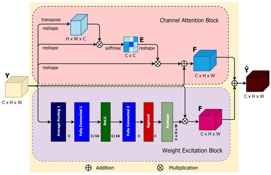
Figure 5.
Illustration of the proposed CAWE block.
Like PAWE, the proposed CAWE block includes two sub-blocks, a channel attention block (CAB) and a weight excitation block (WEB). In the CAB block, the input is reshaped in the initial two steps and permuted in the second part into and , where the superscript c is defined for ”channel”. Afterwards, a matrix multiplication between and is performed. The channel attention map can be defined as:
where the outcome of the ith channel on the jth is produced by . A multiplication of the transposed version of the input feature maps, reshaped to , and the resulting of (5) is performed. Consequently, the final channel attention map can be defined as:
where quantifies the weight of the channel attention map of the input feature map Y. The final WEB sub-network feature map can similarly be obtained from (3).
Finally, an element-wise sum operation is performed between the CAB and WEB output features maps to produce the final CAWE features, as follows:
This process emphasizes generating channel-dependent feature maps using weighted excitation versions of the features of all channels and boosting the feature difference among the channels.
4. Experimental Results and Discussion
4.1. Datasets
In this work, we used two publicly available datasets:
- Lung Image Database Consortium image collection (LIDC-IDRI) [32] consists of 1018 CT scans performed on 1010 patients from 7 different organisations. Each CT scan has been analysed by four radiologists, who individually identified the nodule and manually segmented the region of all the nodules with a diameter larger than three millimetres. Each CT scan can include one or more nodule regions, so the total segmented masks are 5066. Looking closely at the dataset, many nodules are very small and do not satisfy the malignancy index. Therefore, we used a diameter threshold larger than 20 mm to excluded all tiny nodules from our dataset. Afterwards, we split our final dataset, which contains 2044 nodule masks in total, into train, validation and test sets of , , and respectively;
- LUng Nodule Analysis 2016 (LUNA16) [33] is derived from the LIDC-IDRI dataset [32]. It contains 888 CT scans from the LIDC-IDRI dataset for the grand challenge with round annotation masks for all the segmented nodules. The LUNA16 challenge dataset contains 1186 nodule annotations. We obtained 2300 nodule masks from the annotation after pre-processing. We split the dataset into train, validation and test sets similar to the LIDC-IDRI dataset.
4.2. Model Implementation
We individually trained the nodule detection and segmentation models on the PyTorch framework [34]. To train the detection model, the stochastic gradient descent (SGD) [35] optimizer with a learning rate of was used. The binary cross-entropy (BCE) and the norm loss functions were used to train the detection model with a batch size of 4. On the other hand, the Adam [36] optimizer with a learning rate of , as well as the BCE and the IoU loss functions, were also used to train the segmentation model with a batch size of 4. Note that data augmentation was applied during training for both detection and segmentation models to increase the size of the training dataset. We augmented the datasets by random rotation, flipping horizontally and vertically and applying the elastic transform. Finally, all the experiments were carried out on an NVIDIA GeForce GTX 1080 GPU with memory and running about 10–15 h to train 100 epochs for each model.
4.3. Evaluation Measures
Two different procedures were used on both datasets to evaluate the proposed detection and segmentation models. For pixel-level evaluation, the segmentation model provides a pixel-wise output of the class probabilities for every pixel in the input nodule ROIs. The output is converted into a binary segmentation map using a threshold value. Regarding pixel-level evaluation metrics, accuracy (ACC), sensitivity (SEN) and specificity (SPE) are calculated to evaluate the performance of the segmentation model. We also plot a receiver operating characteristic (ROC) curve for calculating area under the curve (AUC). For object-level evaluation, we used the segmentation output to calculate the Dice coefficient (DSC) and intersection over union (IoU) for assessing the ability of the algorithm to previously segment the boundaries of the nodule. Note that in our case, there is no “true negative” class, since there is no “object” corresponding to the absence of nodules. Besides, we also plot the precision-recall (PR) curve instead of the ROC to compare the ground truth number and find the correlation.
4.4. Nodule Detection
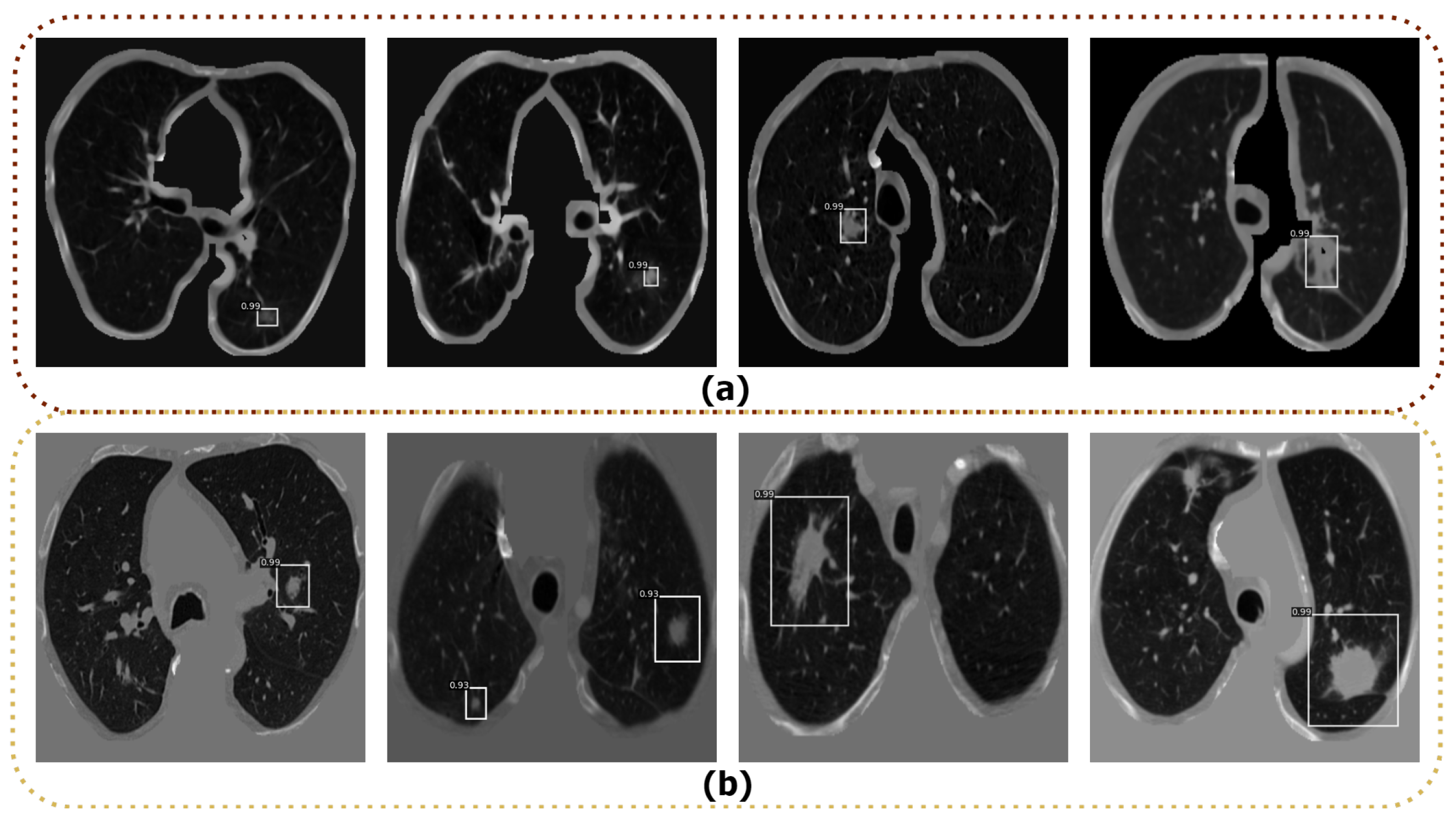
To detect the nodule in the input CT images, we used different state-of-the-art deep learning detector models, such as R-CNN [37], Fast R-CNN [38], original Faster R-CNN [39] and Optimized Faster R-CNN. The aforementioned detection models were trained and tested on the LIDC-IDRI and LUNA16 datasets. To train the above models, we used the data splits as discussed in Section 4.1. We used all default parameters for training the R-CNN [37], Fast-RCNN [38], and original Faster R-CNN [39] models based on their original papers. We fine-tuned the parameters of the original Faster R-CNN to find the best parameters to achieve the highest performance, and named it Optimized Faster R-CNN. The best combination for this model was a learning rate of 0.001, step size of 70,000, gamma of 0.1, and a dropout ratio of 0.5. The model was trained by the pre-trained ResNet50 model to extract the features with a batch size of 64. We finally compared the average precision (AP) of the detection as shown in Table 2 to select the best detection model among the tested models. The Optimized Faster R-CNN model yielded the best results, with the highest AP on both datasets. In turn, R-CNN, Fast R-CNN, original Faster R-CNN models did not properly detect all nodules in the input CT images. Therefore, we have selected the Optimized Faster R-CNN model to detect nodules in CT images. Some examples of lung nodule detection using Optimized Faster R-CNN are shown in Figure 6. As shown, the Optimized Faster R-CNN model is able to detect the nodule regions, even for small nodules.
Table 2.
The average precision (AP) comparison of the four detection models (bold represents the best performance).
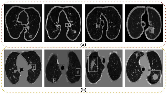
Figure 6.
Examples of lung nodule detection using Optimized Faster R-CNN; (a) Detection results from the LIDC-IDRI dataset; (b) Detection results from the LUNA16 dataset.
4.5. Nodule Segmentation
The proposed lung nodule segmentation model was compared to the state-of-the-art approaches and evaluated in terms of quantitative and qualitative results. For the quantitative study, we used ACC, SEN, and SPE for pixel-level and DSC and IoU for object-level performance, respectively, as shown in Table 3. We compared the AWEU-Net to six different lung nodule segmentation models considering both datasets: PSPNet [40], MANet [41], PAN [42], FPN [43], DeeplabV3 [44], and U-Net [21,22]. As shown in Table 3, the integration of both PAWE and CAWE with the U-Net outperformed the segmentation results of the baseline model (U-Net). In general, AWEU-Net outperforms all tested models in terms of the ACC, SPE, DSC, and IoU metrics on the LUNA16 dataset. AWEU-Net yields ACC, SPE, DSC, and IoU scores of 91.32%, 93.46%, 89.79%, 82.32%, and 89.88%, respectively, which is 1.18%, 1.47%, 0.97%, 1.8%, and 0.93% points higher than the scores of the second-best method (i.e., U-Net). In turn, the DeeplabV3 achieved a SEN score of 93.01%, which is 1.32% points higher than AWEU-Net. However, the proposed segmentation model provides a comparable SEN score of .
Table 3.
Comparison between the proposed AWEU-Net and six other models on the LIDC-IDRI and LUNA16 test datasets (bold represents the best performance).
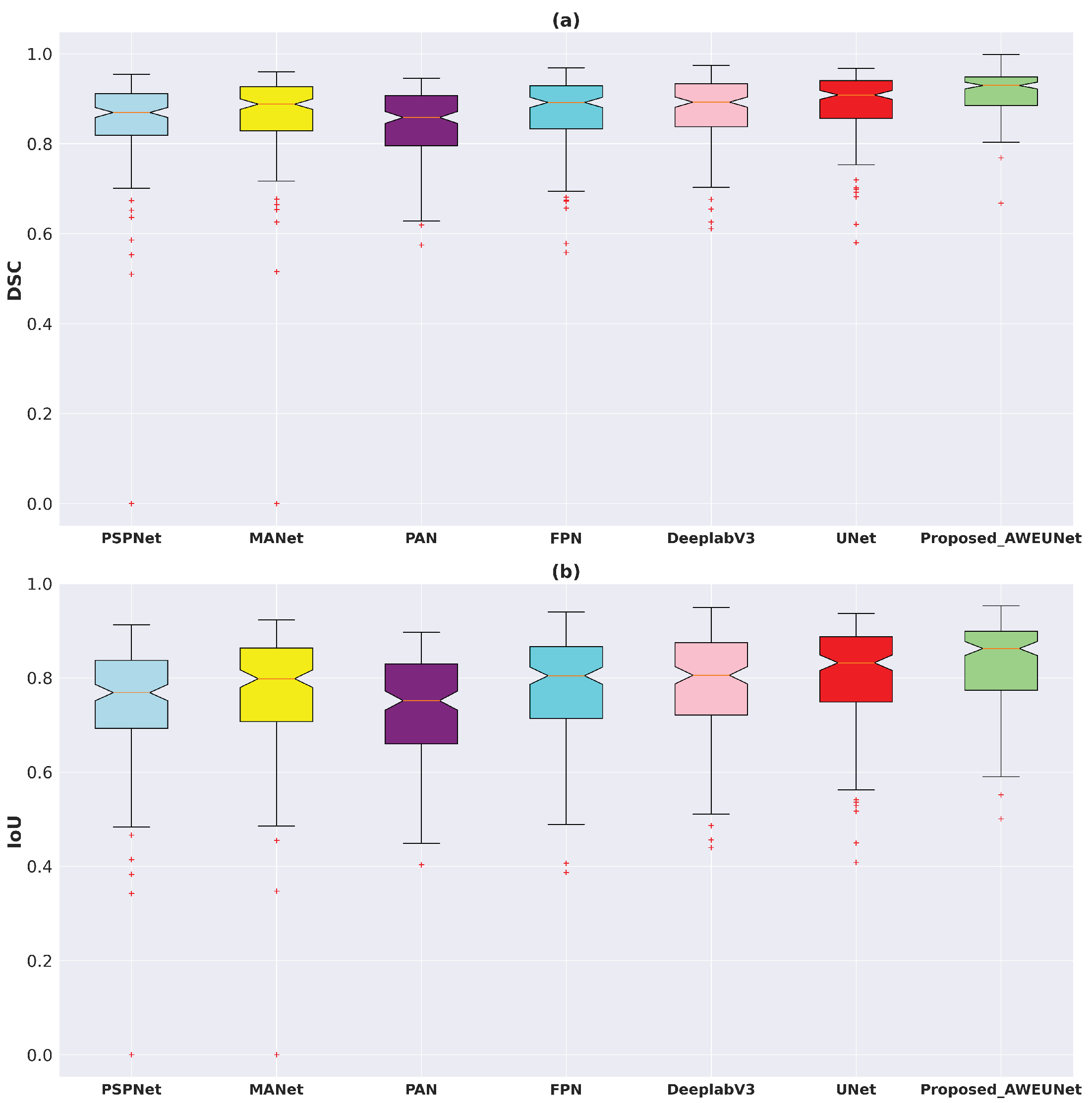
In addition, using the test set of the LUNA16 and LIDC-IDRI datasets, the box plots of DSC and IoU scores of the six models and AWEU-Net were drawn to demonstrate the segmentation ability of AWEU-Net as shown in Figure 7. On both datsets, the proposed AWEU-Net yields higher DSC and IoU mean scores and the lowest standard deviation with only two outliers; this is as compared to the other six segmentation models, which contain many outliers with lower mean and higher standard deviation scores.

Figure 7.
Boxplots of (a) Dice coefficient (DSC) and (b) intersection over union (IoU) scores for all test samples of the LUNA16 lung nodule segmentation dataset. Different boxes indicate the score ranges of several methods; the red line inside each box represents the median value, and all values outside the whiskers are considered outliers, which are marked with the (+) symbol.
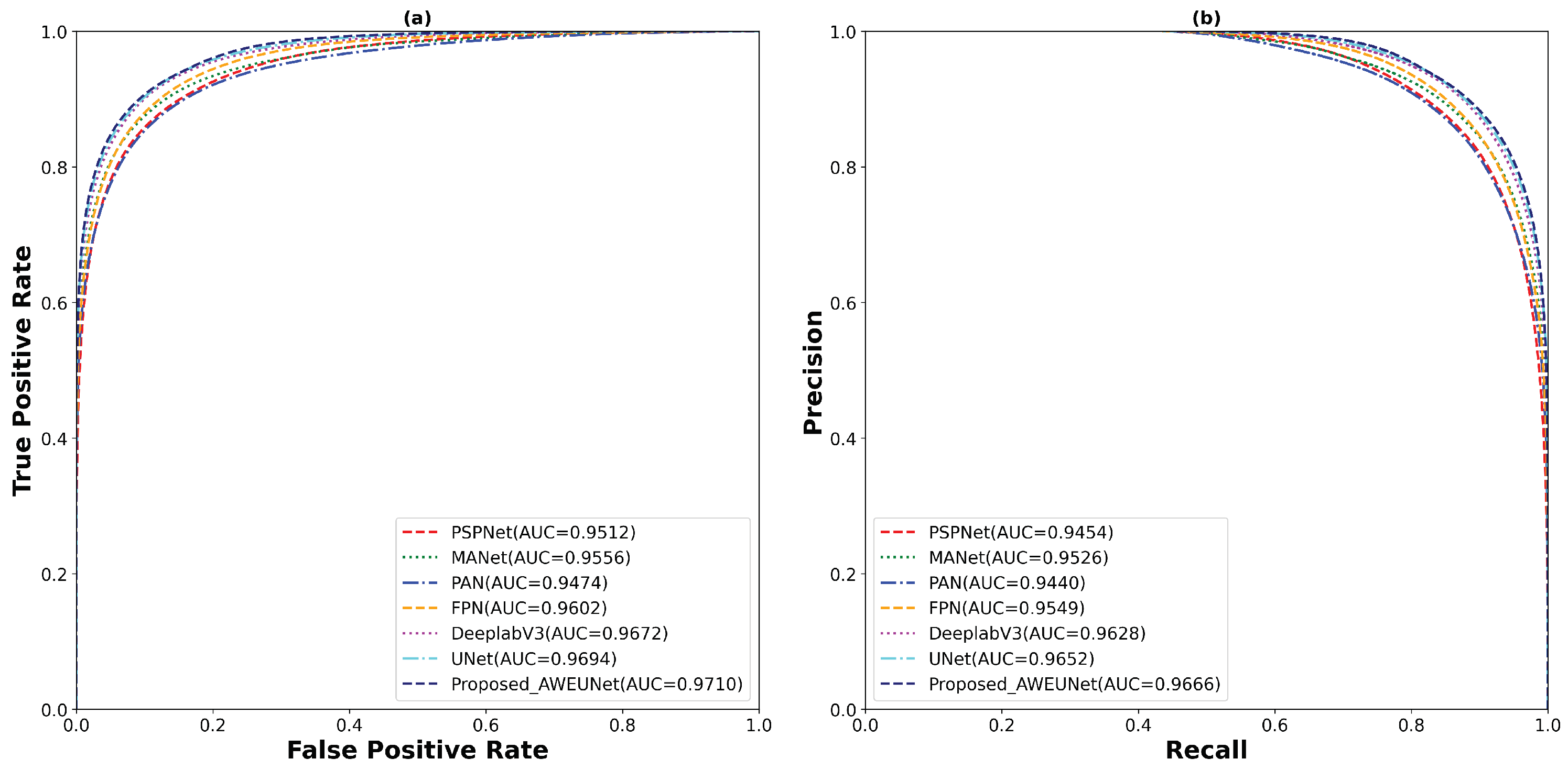
Furthermore, to predict the probability of the binary segmented masks, the ROC and PR curves were constructed as shown in Figure 8. Using the LUNA16 test set, the proposed AWEU-Net model yields the highest AUC and PR of , and , respectively, among the seven segmentation models tested.
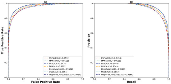
Figure 8.
The (a) ROC and (b) PR curve for all test samples of the LUNA16 lung nodule segmentation dataset.
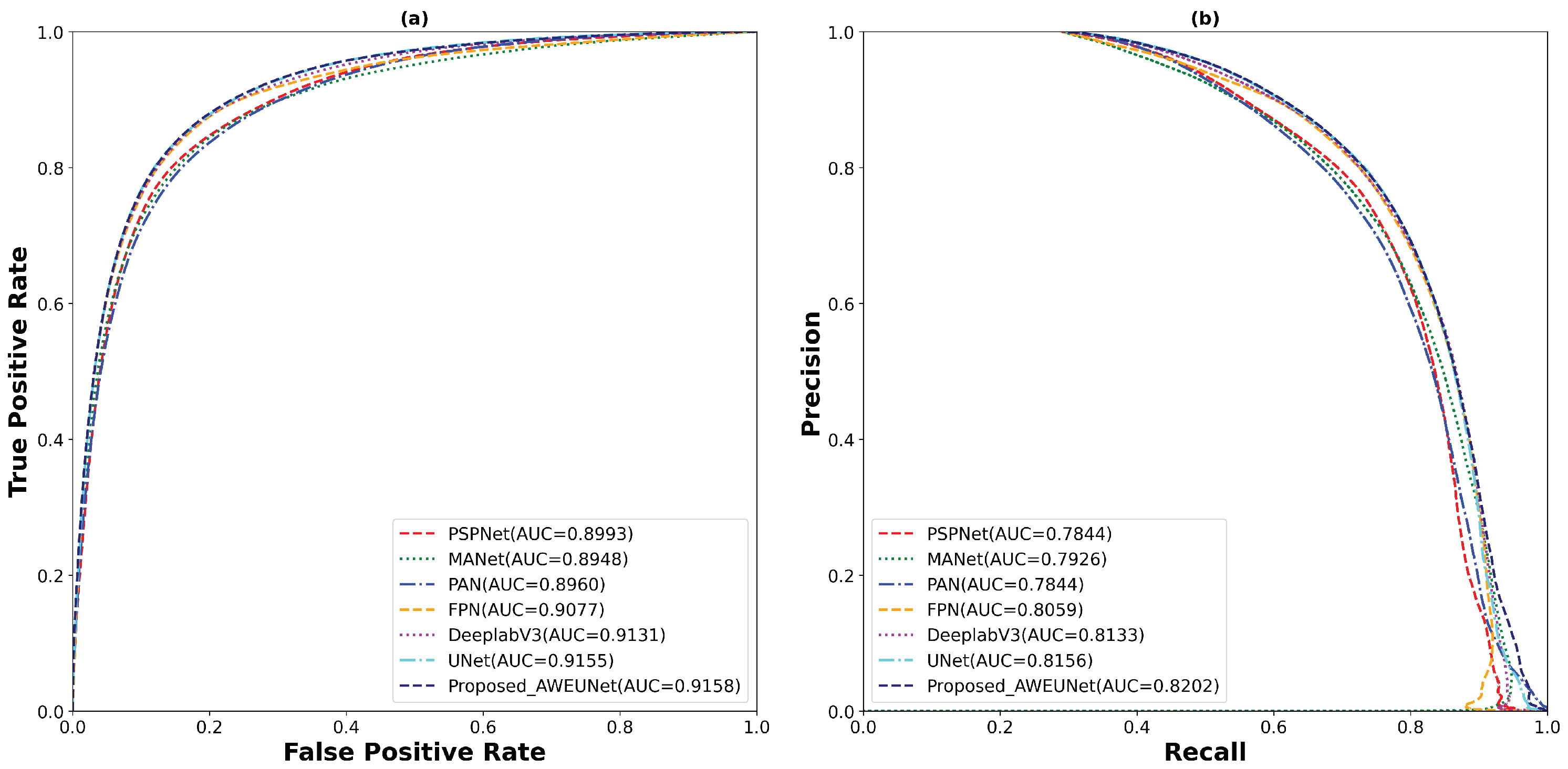
On the other hand, AWEU-Net outperforms all the tested models in terms of all evaluation metrics on the LIDC-IDRI dataset. The proposed model yields ACC, SEN, SPE, DSC, and IoU scores of 94.66%, 90.84%, 96.41%, 90.35%, and 83.21%, respectively. It has improved by 0.3%, 1.16%, 0.06%, 0.48%, and 1.21% in ACC, SEN, SPE, DSC, and IoU scores from the original U-Net. Again, the box plots of DSC and IoU scores of the LIDC-IDRI dataset to compare the models’ performance is displayed in Figure 9. Likewise, the proposed AWEU-Net achieved the highest DSC and IoU mean scores and the smallest standard deviation with only one outlier. The proposed model achieved an AUC of the ROC and PR on the LIDC-IDRI test dataset of 91.58%, and 82.02%, respectively, as shown in Figure 10.
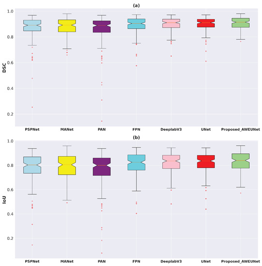
Figure 9.
Boxplots of (a) Dice coefficient (DSC) and (b) intersection over union (IoU) scores for all test samples of the LIDC-IDRI lung nodule segmentation dataset. Different boxes indicate the score ranges of several methods; the red line inside each box represents the median value, and all values outside the whiskers are considered outliers, which are marked with the (+) symbol.
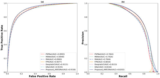
Figure 10.
The (a) ROC and (b) PR curve for for all test samples of the LIDC-IDRI lung nodule segmentation dataset.
A qualitative comparison of the segmentation results of the AWEU-Net and the six segmentation models is shown in Figure 11. The segmentation results of the input nodule ROIs of CT images with a variety of difficult levels, including illumination variations and irregular shapes and boundaries of the nodule regions, were presented. As shown in Figure 11, four examples from the two datasets along with the ground truth and the predicted mask of the six tested models were compared to the proposed AWEU-Net model. AWEU-Net provides segmentation results very close to the ground truth with an average similarity of >86% (true positive (TP)). Our segmentation method also provides the lowest degrees of false negative (FN) and false positive (FP) results compared to the rest of the models. The AWEU-Net model yields more regular borders compared to PSPNet, MANet, FPN, since our model strives for higher accuracy on nodule region boundaries. The resulting segmentation of the six tested models may significantly differ from the ground truth in some cases, e.g., the second example of the LUNA16 dataset.
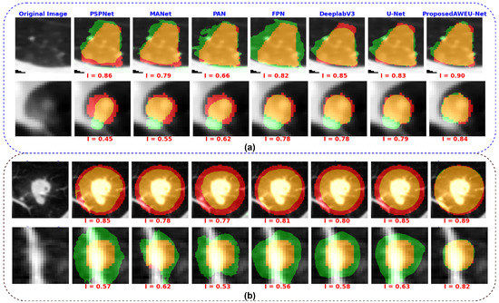
Figure 11.
Examples of segmentation results by different state-of-the-art models. (a) Segmentation results on the LIDC-IDRI dataset and (b) segmentation results on the LUNA16 dataset. The colors of the segmentation visualization results are presented as follows: TP (orange), TN (background), FP (green), and FN (red).
Finally, regarding the model efficiency, the total number of parameters, the sum of all the weights and biases on the proposed model, was around 34.5 million. Our model yielded a reduction of compared to the baseline model, UNet (i.e., number of parameters of around 60 million). In order to assess the computational complexity of the model, we measured the number of resources that the proposed model used in training and inference by computing the multiply-accumulate operation (MACs) in billions of operations, (MACs(G)). The proposed model performed 65.3 billion MACs. Furthermore, our proposed model achieved an inference time of 10.8 ms (around 92.3 fps) on an NVIDIA GeForce GTX 1080 GPU. In summary, our framework can be executed on a single GPU, guaranteeing accurate nodule segmentation in real-time.
5. Conclusions
This article proposed a reliable system for lung nodule detection and segmentation. The system contains two deep learning models. Firstly, the Optimized Faster R-CNN model [39] trained with lung CT scan images was used for detecting the nodule region in a CT image as an initial step. Secondly, a segmentation model, AWEU-Net, was proposed for segmenting the nodule boundaries of the detected nodule region. The proposed segmentation model, AWEU-Net, includes PAWE and CAWE blocks to improve the segmentation performance. Compared to the state-of-the-art models, the proposed AWEU-Net model yields the best segmentation accuracy with DSC and IoU scores of , , and , on the LUNA16 and LIDC-IDRI datasets, respectively. Although the proposed method provided promising nodule segmentation results, the number of parameters of the segmentation model is a bit high (around 34.5 million). Thus, it is not appropriate for computing devices with limited resources. Consequently, ongoing work will aim at developing a lightweight nodule segmentation model. In future work, we will develop a comprehensive nodule segmentation system, and it will be able to classify and grade nodule malignancy.
Author Contributions
Conceptualization, S.F.B. and M.M.K.S.; methodology, S.F.B. and M.M.K.S.; software, S.F.B. and M.M.K.S.; validation, S.F.B. and M.M.K.S.; formal analysis, S.F.B. and M.M.K.S.; investigation, S.F.B. and M.M.K.S.; resources, S.F.B. and M.M.K.S.; data curation, S.F.B. and M.M.K.S.; writing—original draft preparation, S.F.B. and M.M.K.S.; writing—review and editing, S.F.B., M.M.K.S., M.A.-N. and H.A.R.; visualization, S.F.B. and M.M.K.S.; supervision, M.A.-N., D.P. and H.A.R.; project administration, M.A.-N., D.P. and H.A.R.; funding acquisition, M.A.-N., D.P. and H.A.R.; All authors have read and agreed to the published version of the manuscript.
Funding
This research received no external funding.
Institutional Review Board Statement
The study was approved by URV.
Informed Consent Statement
Not applicable.
Data Availability Statement
The samples used are publicly available.
Acknowledgments
The Spanish Government partly supported this research through project PID2019-105789RB-I00.
Conflicts of Interest
All authors declare no conflict of interest.
Abbreviations
The following abbreviations are used in this manuscript:
| CAD | Computer-aided Diagnosis |
| CADe | Computer-aided Detection |
| CASe | Computer-aided Segmentation |
| CT | Computed Tomography |
| AI | Artificial Intelligence |
| GMM | Gaussian Mixture Model |
| CNNs | Convolutional Neural Networks |
| R-CNN | Region-based Convolutional Neural Network |
| ROI | Region of Interest (ROI) |
| RPN | Region Proposal Network |
| FPN | Feature Pyramid Network |
| ReLU | Rectified Linear Unit |
| SGD | Stochastic Gradient Descent |
| BCE | Binary Cross-Entropy |
| Dice | Dice Coefficient |
| IoU | Intersection Over Union |
| ROC | Receiver Operating Characteristic |
| AUC | Area Under the Curve |
| ACC | Accuracy |
| SEN | Sensitivity |
| SPE | Specificity |
| GPU | Graphics Processing Unit |
| GB | Gigabytes |
| DL | Deep Learning |
References
- Cancer. Available online: https://www.who.int/news-room/fact-sheets/detail/cancer/ (accessed on 8 August 2021).
- World Lung Cancer Day 2020 Fact Sheet. Available online: https://www.chestnet.org/newsroom/chest-news/2020/07/world-lung-cancer-day-2020-fact-sheet/ (accessed on 8 August 2021).
- The National Lung Screening Trial Research Team. Reduced lung-cancer mortality with low-dose computed tomographic screening. N. Engl. J. Med. 2011, 365, 395–409. [Google Scholar] [CrossRef] [PubMed] [Green Version]
- Yu, K.H.; Lee, T.L.M.; Yen, M.H.; Kou, S.; Rosen, B.; Chiang, J.H.; Kohane, I.S. Reproducible Machine Learning Methods for Lung Cancer Detection Using Computed Tomography Images: Algorithm Development and Validation. J. Med. Internet Res. 2020, 22, e16709. [Google Scholar] [CrossRef] [PubMed]
- Seattle Cancer Care Alliance Proton Therapy Center. Available online: https://www.sccaprotontherapy.com/cancers-treated/lung-cancer-treatment (accessed on 8 August 2021).
- Callister, M.; Baldwin, D.; Akram, A.; Barnard, S.; Cane, P.; Draffan, J.; Franks, K.; Gleeson, F.; Graham, R.; Malhotra, P.; et al. British Thoracic Society guidelines for the investigation and management of pulmonary nodules: Accredited by NICE. Thorax 2015, 70, ii1–ii54. [Google Scholar] [CrossRef] [Green Version]
- Aresta, G.; Jacobs, C.; Araújo, T.; Cunha, A.; Ramos, I.; van Ginneken, B.; Campilho, A. iW-Net: An automatic and minimalistic interactive lung nodule segmentation deep network. Sci. Rep. 2019, 9, 11591. [Google Scholar] [CrossRef] [PubMed] [Green Version]
- Keetha, N.V.; Babu P, S.A.; Annavarapu, C.S.R. U-Det: A Modified U-Net architecture with bidirectional feature network for lung nodule segmentation. arXiv 2020, arXiv:2003.09293. [Google Scholar]
- Cao, H.; Liu, H.; Song, E.; Hung, C.C.; Ma, G.; Xu, X.; Jin, R.; Lu, J. Dual-branch residual network for lung nodule segmentation. Appl. Soft Comput. 2020, 86, 105934. [Google Scholar] [CrossRef]
- Wu, B.; Zhou, Z.; Wang, J.; Wang, Y. Joint learning for pulmonary nodule segmentation, attributes and malignancy prediction. In Proceedings of the 2018 IEEE 15th International Symposium on Biomedical Imaging (ISBI 2018), Washington, DC, USA, 4–7 April 2018; pp. 1109–1113. [Google Scholar]
- Tang, H.; Zhang, C.; Xie, X. Nodulenet: Decoupled false positive reduction for pulmonary nodule detection and segmentation. In Proceedings of the 22nd International Conference on Medical Image Computing and Computer-Assisted Intervention, Shenzhen, China, 13–17 October 2019; pp. 266–274. [Google Scholar]
- Kumar Singh, V.; Abdel-Nasser, M.; Pandey, N.; Puig, D. Lunginfseg: Segmenting COVID-19 infected regions in lung ct images based on a receptive-field-aware deep learning framework. Diagnostics 2021, 11, 158. [Google Scholar] [CrossRef]
- Jiang, J.; Hu, Y.-C.; Liu, C.J.; Halpenny, D.; Hellmann, M.D.; Deasy, J.O.; Mageras, G.; Veeraraghavan, H. Multiple resolution residually connected feature streams for automatic lung tumor segmentation from CT images. IEEE Trans. Med. Imaging 2018, 38, 134–144. [Google Scholar] [CrossRef]
- Dehmeshki, J.; Amin, H.; Valdivieso, M.; Ye, X. Segmentation of pulmonary nodules in thoracic CT scans: A region growing approach. IEEE Trans. Med. Imaging 2008, 27, 467–480. [Google Scholar] [CrossRef] [Green Version]
- Tan, Y.; Schwartz, L.H.; Zhao, B. Segmentation of lung lesions on CT scans using watershed, active contours, and Markov random field. Med. Phys. 2013, 40, 043502. [Google Scholar] [CrossRef] [Green Version]
- Farag, A.A.; Abd El Munim, H.E.; Graham, J.H.; Farag, A.A. A novel approach for lung nodules segmentation in chest CT using level sets. IEEE Trans. Image Process. 2013, 22, 5202–5213. [Google Scholar] [CrossRef]
- Dai, S.; Lu, K.; Dong, J.; Zhang, Y.; Chen, Y. A novel approach of lung segmentation on chest CT images using graph cuts. Neurocomputing 2015, 168, 799–807. [Google Scholar] [CrossRef]
- Navya, K.; Pradeep, G. Lung Nodule Segmentation Using Adaptive Thresholding and Watershed Transform. In Proceedings of the 2018 3rd IEEE International Conference on Recent Trends in Electronics, Information & Communication Technology (RTEICT), Bangalore, India, 18–19 May 2018; pp. 630–633. [Google Scholar]
- Li, X.; Li, B.; Liu, F.; Yin, H.; Zhou, F. Segmentation of pulmonary nodules using a GMM fuzzy C-means algorithm. IEEE Access 2020, 8, 37541–37556. [Google Scholar] [CrossRef]
- Savic, M.; Ma, Y.; Ramponi, G.; Du, W.; Peng, Y. Lung nodule segmentation with a region-based fast marching method. Sensors 2021, 21, 1908. [Google Scholar] [CrossRef]
- Skourt, B.A.; El Hassani, A.; Majda, A. Lung CT image segmentation using deep neural networks. Procedia Comput. Sci. 2018, 127, 109–113. [Google Scholar] [CrossRef]
- Ronneberger, O.; Fischer, P.; Brox, T. U-net: Convolutional networks for biomedical image segmentation. In Proceedings of the 18th International Conference on Medical Image Computing and Computer-Assisted Intervention, Munich, Germany, 5–9 October 2015; pp. 234–241. [Google Scholar]
- He, K.; Zhang, X.; Ren, S.; Sun, J. Deep residual learning for image recognition. In Proceedings of the IEEE Conference on Computer Vision and Pattern Recognition, Las Vegas, NV, USA, 27–30 June 2016; pp. 770–778. [Google Scholar]
- Misra, D. Mish: A self regularized non-monotonic neural activation function. arXiv 2019, arXiv:1908.08681. [Google Scholar]
- Hancock, M.C.; Magnan, J.F. Lung nodule malignancy classification using only radiologist-quantified image features as inputs to statistical learning algorithms: Probing the Lung Image Database Consortium dataset with two statistical learning methods. J. Med. Imaging 2016, 3, 044504. [Google Scholar] [CrossRef] [Green Version]
- Lin, T.Y.; Maire, M.; Belongie, S.; Hays, J.; Perona, P.; Ramanan, D.; Dollár, P.; Zitnick, C.L. Microsoft coco: Common objects in context. In Proceedings of the 13th European Conference on Computer Vision, Zurich, Switzerland, 6–12 September 2014; pp. 740–755. [Google Scholar]
- Huang, J.; Rathod, V.; Sun, C.; Zhu, M.; Korattikara, A.; Fathi, A.; Fischer, I.; Wojna, Z.; Song, Y.; Guadarrama, S.; et al. Speed/accuracy trade-offs for modern convolutional object detectors. In Proceedings of the IEEE Conference on Computer Vision and Pattern Recognition, Honolulu, HI, USA, 21–26 July 2017; pp. 7310–7311. [Google Scholar]
- Zeren, M.T.; Aytulun, S.K.; Kırelli, Y. Comparison of SSD and faster R-CNN algorithms to detect the airports with data set which obtained from unmanned aerial vehicles and satellite images. Avrupa Bilim ve Teknoloji Dergisi 2020, 643–658. [Google Scholar] [CrossRef]
- Fu, J.; Liu, J.; Tian, H.; Li, Y.; Bao, Y.; Fang, Z.; Lu, H. Dual attention network for scene segmentation. In Proceedings of the IEEE Conference on Computer Vision and Pattern Recognition, Long Beach, CA, USA, 15–20 June 2019; pp. 3146–3154. [Google Scholar]
- Peng, C.; Zhang, X.; Yu, G.; Luo, G.; Sun, J. Large kernel matters–improve semantic segmentation by global convolutional network. In Proceedings of the IEEE Conference on Computer Vision and Pattern Recognition, Honolulu, HI, USA, 21–26 July 2017; pp. 4353–4361. [Google Scholar]
- Quader, N.; Bhuiyan, M.M.I.; Lu, J.; Dai, P.; Li, W. Weight Excitation: Built-in Attention Mechanisms in Convolutional Neural Networks. In Proceedings of the 16th European Conference on Computer Vision, Glasgow, UK, 23–28 August 2020; pp. 87–103. [Google Scholar]
- Armato, S.G., III; McLennan, G.; Bidaut, L.; McNitt-Gray, M.F.; Meyer, C.R.; Reeves, A.P.; Zhao, B.; Aberle, D.R.; Henschke, C.I.; Hoffman, E.A.; et al. The lung image database consortium (LIDC) and image database resource initiative (IDRI): A completed reference database of lung nodules on CT scans. Med. Phys. 2011, 38, 915–931. [Google Scholar]
- Setio, A.A.A.; Traverso, A.; De Bel, T.; Berens, M.S.; Van Den Bogaard, C.; Cerello, P.; Chen, H.; Dou, Q.; Fantacci, M.E.; Geurts, B.; et al. Validation, comparison, and combination of algorithms for automatic detection of pulmonary nodules in computed tomography images: The LUNA16 challenge. Med. Image Anal. 2017, 42, 1–13. [Google Scholar] [CrossRef] [Green Version]
- Paszke, A.; Gross, S.; Massa, F.; Lerer, A.; Bradbury, J.; Chanan, G.; Killeen, T.; Lin, Z.; Gimelshein, N.; Antiga, L.; et al. Pytorch: An imperative style, high-performance deep learning library. Adv. Neural Inf. Process. Syst. 2019, 32, 8026–8037. [Google Scholar]
- Gulcehre, C.; Sotelo, J.; Bengio, Y. A robust adaptive stochastic gradient method for deep learning. In Proceedings of the 2017 International Joint Conference on Neural Networks (IJCNN), Anchorage, AK, USA, 14–19 May 2017; pp. 125–132. [Google Scholar]
- Kingma, D.P.; Ba, J. Adam: A method for stochastic optimization. arXiv 2014, arXiv:1412.6980. [Google Scholar]
- Girshick, R.; Donahue, J.; Darrell, T.; Malik, J. Rich feature hierarchies for accurate object detection and semantic segmentation. In Proceedings of the IEEE Conference on Computer Vision and Pattern Recognition, Columbus, OH, USA, 23–28 June 2014; pp. 580–587. [Google Scholar]
- Girshick, R. Fast r-cnn. In Proceedings of the IEEE International Conference on Computer Vision, Santiago, Chile, 7–13 December 2015; pp. 1440–1448. [Google Scholar]
- Ren, S.; He, K.; Girshick, R.; Sun, J. Faster R-CNN: Towards real-time object detection with region proposal networks. IEEE Trans. Pattern Anal. Mach. Intell. 2016, 39, 1137–1149. [Google Scholar] [CrossRef] [PubMed] [Green Version]
- Zhao, H.; Shi, J.; Qi, X.; Wang, X.; Jia, J. Pyramid scene parsing network. In Proceedings of the IEEE Conference on Computer Vision and Pattern Recognition, Honolulu, HI, USA, 21–26 July 2017; pp. 2881–2890. [Google Scholar]
- Fan, T.; Wang, G.; Li, Y.; Wang, H. Ma-net: A multi-scale attention network for liver and tumor segmentation. IEEE Access 2020, 8, 179656–179665. [Google Scholar] [CrossRef]
- Li, H.; Xiong, P.; An, J.; Wang, L. Pyramid attention network for semantic segmentation. arXiv 2018, arXiv:1805.10180. [Google Scholar]
- Lin, T.Y.; Dollár, P.; Girshick, R.; He, K.; Hariharan, B.; Belongie, S. Feature pyramid networks for object detection. In Proceedings of the IEEE Conference on Computer Vision and Pattern Recognition, Honolulu, HI, USA, 21–26 July 2017; pp. 2117–2125. [Google Scholar]
- Chen, L.C.; Papandreou, G.; Schroff, F.; Adam, H. Rethinking atrous convolution for semantic image segmentation. arXiv 2017, arXiv:1706.05587. [Google Scholar]


Publisher’s Note: MDPI stays neutral with regard to jurisdictional claims in published maps and institutional affiliations. |
© 2021 by the authors. Licensee MDPI, Basel, Switzerland. This article is an open access article distributed under the terms and conditions of the Creative Commons Attribution (CC BY) license (https://creativecommons.org/licenses/by/4.0/).