Machine Learning Based on Resampling Approaches and Deep Reinforcement Learning for Credit Card Fraud Detection Systems

Abstract

The problem of imbalanced datasets is a significant concern when creating reliable credit card fraud (CCF) detection systems. In this work, we study and evaluate recent advances in machine learning (ML) algorithms and deep reinforcement learning (DRL) used for CCF detection systems, including fraud and non-fraud labels. Based on two resampling approaches, SMOTE and ADASYN are used to resample the imbalanced CCF dataset. ML algorithms are, then, applied to this balanced dataset to establish CCF detection systems. Next, DRL is employed to create detection systems based on the imbalanced CCF dataset. The diverse classification metrics are indicated to thoroughly evaluate the performance of these ML and DRL models. Through empirical experiments, we identify the reliable degree of ML models based on two resampling approaches and DRL models for CCF detection. When SMOTE and ADASYN are used to resampling original CCF datasets before training/test split, the ML models show very high outcomes of above 99% accuracy. However, when these techniques are employed to resample for only the training CCF datasets, these ML models show lower results, particularly in terms of logistic regression with 1.81% precision and 3.55% F1 score for using ADASYN. Our work reveals the DRL model is ineffective and achieves low performance, with only 34.8% accuracy.

1. Introduction

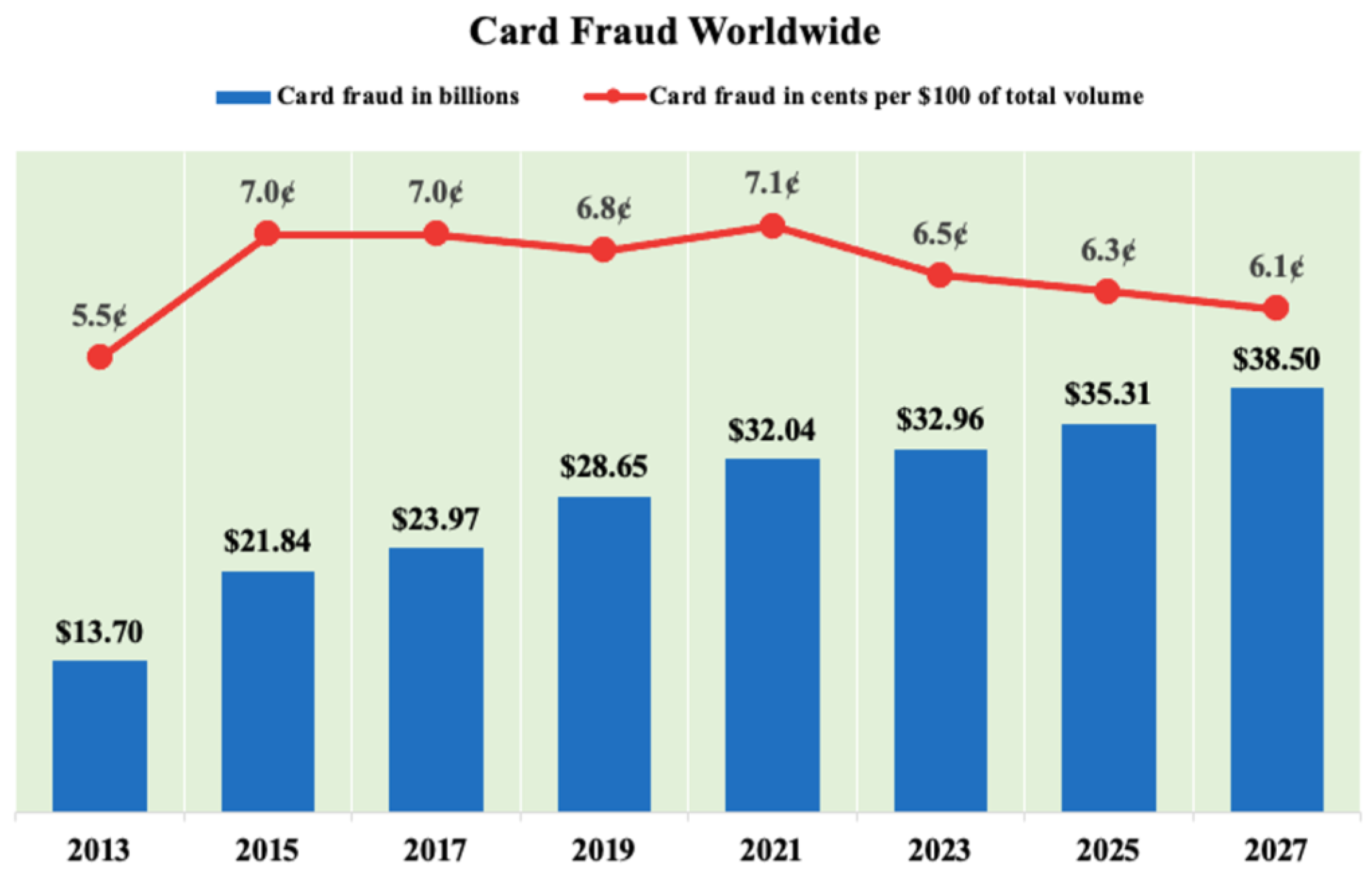
In the fourth industrial revolution, the e-commerce platform has become the most extensive system for financial institutions. People tend to select services of e-commerce and the Internet to enhance productivity and mitigate time-consuming tasks. Online transactions are becoming increasingly popular. Therefore, fraudulent activities have been increasing significantly in various industries worldwide, particularly in the financial industry. In financial companies, credit card fraud (CCF) is considered as the most problematic form of fraud and there is a need to develop tools to prevent it as soon as possible. Figure 1 indicates a summary of the total number of CCF and cents lost per 100 dollars from 2013 to 2027 worldwide [1]. The total number of CCF has increased significantly, from approximately $13.7 billion in 2013 to about $38.5 billion in 2027 globally. In the year 2021, the total CCF are predicted to lose $32.4 billion, amounting to 7.1 cents per $100 of the total volume. In order to dramatically reduce the consequences of CCF, fraud detection approaches need to be investigated in order to strictly handle it. Typically, the detection systems of CCF are trained through previous transactions to determine upcoming ones [2].

Figure 1. Card fraud worldwide from 2010 to 2027 [1].

In CCF identification, the number of fraudulent cases is significantly less than under normal circumstances. This leads to the status of the imbalanced dataset. In this CCF imbalanced dataset, one class of dataset has an extremely high number of instances, while the other class accounts for only a very small number of instances. However, machine learning (ML) algorithms work effectively on the balanced distribution of classes. In order to tackle the issue of imbalanced datasets, various remedies have been researched in the past decades. In the research, three groups, known as the data-level, algorithm-level, and ensemble solutions, are commonly proposed [3].

Additionally, the deep reinforcement learning (DRL) approach has recently emerged as an effective approach for classifying imbalances. The classification problem is formulated as a sequential decision-making process and is handled via a deep Q-learning network. A classification action on one sample is performed by an agent at each time step. The classification action is evaluated through the environment and the agent receives a reward. The minority class sample receives a large reward, so the agent is more susceptible to this class. The agent eventually searches for an optimal classification policy in the imbalanced dataset based on a specific reward function and a beneficial learning environment. This approach is applied directly to several datasets, such as the modified national institute of standards and technology (MNIST) database, and the internet movie database (IMDB), and its effective performance has been demonstrated [4].

In [5], two resampling techniques, named the synthetic minority oversampling technique (SMOTE) and adaptive synthetic (ADASYN), were used to obtain the balanced CCF dataset. The machine learning (ML) algorithms, named random forest (RF), k nearest neighbors (KNN), decision tree (DT), and logistic regression (LR), were then utilized to train the balanced CCF dataset obtained from SMOTE and ADASYN. The comparison of the performance of these ML algorithms, based on these resampling techniques, was used to indicate the best case for detecting CCF. However, this study did not provide diverse algorithms to handle imbalanced CCF datasets.

This research is an extension of our previous work [5]. In this research, we expand the DRL approach and include three more effective ML classifiers, such as adaptive boosting (AdaBoost), eXtreme Gradient Boosting (XGBoost), and deep neural network (DNN) in order to have diverse solutions to comprehensively develop the CCF detection systems. Furthermore, we develop the comparison of the performance of the DRL approach applied directly to the CCF imbalanced dataset and ML classifiers based on the resampling of the CCF dataset in order to analyze the contributions and limitations of the models related to the ML field for the CCF detection systems. The primary contributions of this research are fourfold:

-

Implementing the processing data for the imbalanced CCF dataset to increase the performance of classification between fraud and non-fraud labels. SMOTE and ADASYN techniques are used to resample this imbalanced CCF dataset based on two resampling approaches.

-

Reviewing and discussing in-depth the classification measurement indexes which can be employed to deal with the problem of the accuracy paradox for the CCF detection ML models.

-

Applying the seven ML algorithms, i.e., KNN, LR, DT, RF, AdaBoost, XGBoost, and DNN, to the balanced CCF dataset obtained based on two resampling approaches in order to establish the CCF detection systems. The comparison of the results of the ML models based on these two resampling approaches is indicated to demonstrate the degree of reliability of each approach.

-

Implementing and evaluating the DRL approach on the imbalanced CCF dataset to indicate its reliability. We propose suitable algorithms for dealing with the imbalanced dataset effectively for the CCF detection systems.

The remainder of this study is described as follows: Section 2 depicts related work. Section 3 is about the description of approaches for the imbalanced CCF dataset. Section 4 presents the resampling techniques. Section 5 describes the ML algorithms and the classification metrics. Section 6 shows the DRL method for imbalanced classification. Section 7 illustrates the classification outcomes. Lastly, Section 8 gives concluding remarks and describes future works.

2. Related Work

The data imbalance presents various challenges to performing data analysis and data mining in most real-world research areas, especially online banking transactions. Credit card fraud has resulted in a huge loss for both customers and financial companies worldwide. Therefore, researchers are searching for optimized methods to detect and prevent this fraud. Recently, ML approaches have been applied to detect CCF activities. In [6], the novel approach, named extreme outlier elimination utilizing k reverse nearest neighbors (kRNNs) with hybrid sampling technique, was proposed to generate reliable anticipations to not only fraud but also non-fraud circumstances. This novel approach proved its festiveness compared with other classifiers, such as C4.5, Naive Bayes (NB), KNN, and Radial Basis Function (RBF) networks.

In [7], several ensemble classifiers were analyzed comprehensively through regression and voting for CCF detection. These classifiers were then compared with effective single classifiers, such as KNN, NB, Support Vector Machine (SVM), DT, RBF, and Multilayer Perceptron (MLP). These algorithms were evaluated based on three different datasets that were treated using SMOTE. In [2], the SMOTE-edited nearest neighbor (ENN) method was found to be best for detecting the CCF compared with other different classifiers among a set of oversampling approaches, and the SMOTE-Tomek’s Links (TL) showed good outcomes according to the set of under-sampling techniques. In [8], the combined probabilistic and neuro-adaptive method was proposed to an identified database of credit card transactions. This combination illustrated a high classification of fraud.

In [9], a hidden Markov model (HMM) was employed to create a model of the operations sequences in credit card transaction processing and showed how it was used for the identification of frauds. Through experiment results, the system based on HMM demonstrated its effectiveness and usefulness of learning expenditure profile of the cardholders. The accuracy of this system was about 80% over a wide variation in the input data. The system was also scalable to cope with massive volumes of transactions. In [10], the ML methods were used to detect anomalies in Fintech applications. The suspicious activity in the financial dataset was targeted and the models were created to predict future frauds. The available techniques of anomaly detection were also debated and showed good performance in the CCF detection.

The study [11] proposed a novel hybrid approach with Dynamic Weighted Entropy (DWE) to solve the problem of class imbalance with the overlap in CCF detection, relying on a divide-and-conquer idea. In this study, a new measurement, named DWE, was developed to assist the hyper-parameters selection of the model. With the help of DWE, the model efficiency was improved, and the time consumption on finding good hyper-parameters was exceptionally decreased. Compared with other state-of-the-art methods, this method was proved to be effective through various experiments.

In [12], based on the enhanced R-value, the strategy was developed to select features that ensure that the data achieve minimal overlap, thus improving the performance of the classifier for CCF detection. Three feature selection algorithms, which are Reduce Overlapping with No-sampling (RONS), Reduce Overlapping with SMOTE (ROS), and Reduce Overlapping with ADASYN (ROA), were used to mitigate the overlap degree. The outcomes indicated that the RONS algorithm was successful in detecting the vital features in model selection, whereas both ROS and ROA achieved significantly high performance in terms of the F-measure and G-mean. The effective feature selection strategy was extended as an alternative for tackling problems of class-imbalanced learning involving overlapping.

In summary, there has been a variety of ways to create models for identifying CCF activities to reduce risks in the financial sector. In [10], several modern techniques based on machine learning, data mining, sequence alignment, fuzzy logic, and genetic programming were analyzed to detect credit card fraud. However, depending on each specific case, the techniques mentioned in this study have had different strengths and weaknesses. In [13], a study of imbalanced classification methods was reviewed for the credit fraudulent activities in the experiment. This study indicated that using unbalanced classification approaches was not effective and sufficient to cope with the imbalanced data problem. Moreover, the ML algorithms were applied to the imbalanced CCF dataset, but the classifiers did not detect true positive and true negative values in several circumstances [14]. Additionally, the classification accuracy criterion did not effectively and comprehensively evaluate the ML models, resulting in the accuracy paradox in several circumstances for CCF detection systems [15,16]. In this research, we provide the study-in-depth of ML/DRL for the imbalanced datasets, especially the imbalanced CCF dataset.

3. Approaches for Imbalanced Datasets

3.1. Dataset

In this study, we select the dataset of CCF prediction as a case study of the imbalanced dataset obtained in [17]. The description of this dataset is shown in Table 1. In September 2013, this dataset included transactions that were collected within 2 days and created by credit cards through European cardholders. The imbalanced CCF dataset has 284,807 transactions and 31 columns. These columns consist of 28 numerical features, named V1 to V28, a feature of “Time”, a feature of “Amount”, and a label of “Class”. The label of “Class” is divided into two classes, such as positive class (frauds), denoted as 1, and negative class (no-frauds), denoted as 0. The type of all of these features is expressed as an object, and there are no missing values in this dataset.

Table 1. Data description.

Descriptions	Details
Number of columns	31
Number of features	30
Labels	Class 0 and class 1
Number of rows	284,807
Feature type	Object
Missing values	None
No frauds vs Frauds	99.828% vs. 0.172%

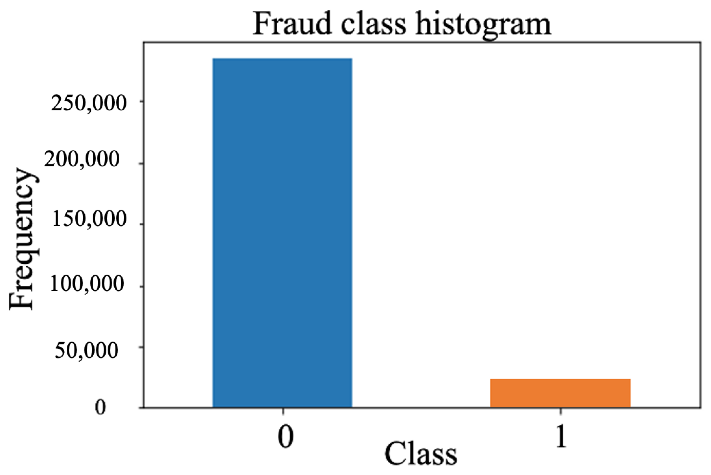
As shown in Figure 2, this CCF dataset is highly imbalanced so we can define the positive and negative classes as the minority and the majority classes. It is true that the imbalanced ratio (IR) is the most prevalently employed measure, which illustrates the imbalanced extent of a dataset.

Figure 2. Fraud class histogram with the imbalanced dataset.

This ratio is considered as a ratio of the sample size of the majority class $N_{maj}$ over the sample size of the minority one $N_{min}$, as shown in (1). If the IR value is equal to 1, the dataset is exactly balanced between two classes. If the IR value is bigger than 1, we have an imbalanced dataset [18]. In the CCF dataset of this paper, the minority class (frauds) occupied only 0.172% of all transactions, as illustrated in Figure 2.

$$\mathrm{IR}=\frac{N_{maj}}{N_{min}}$$

(1)

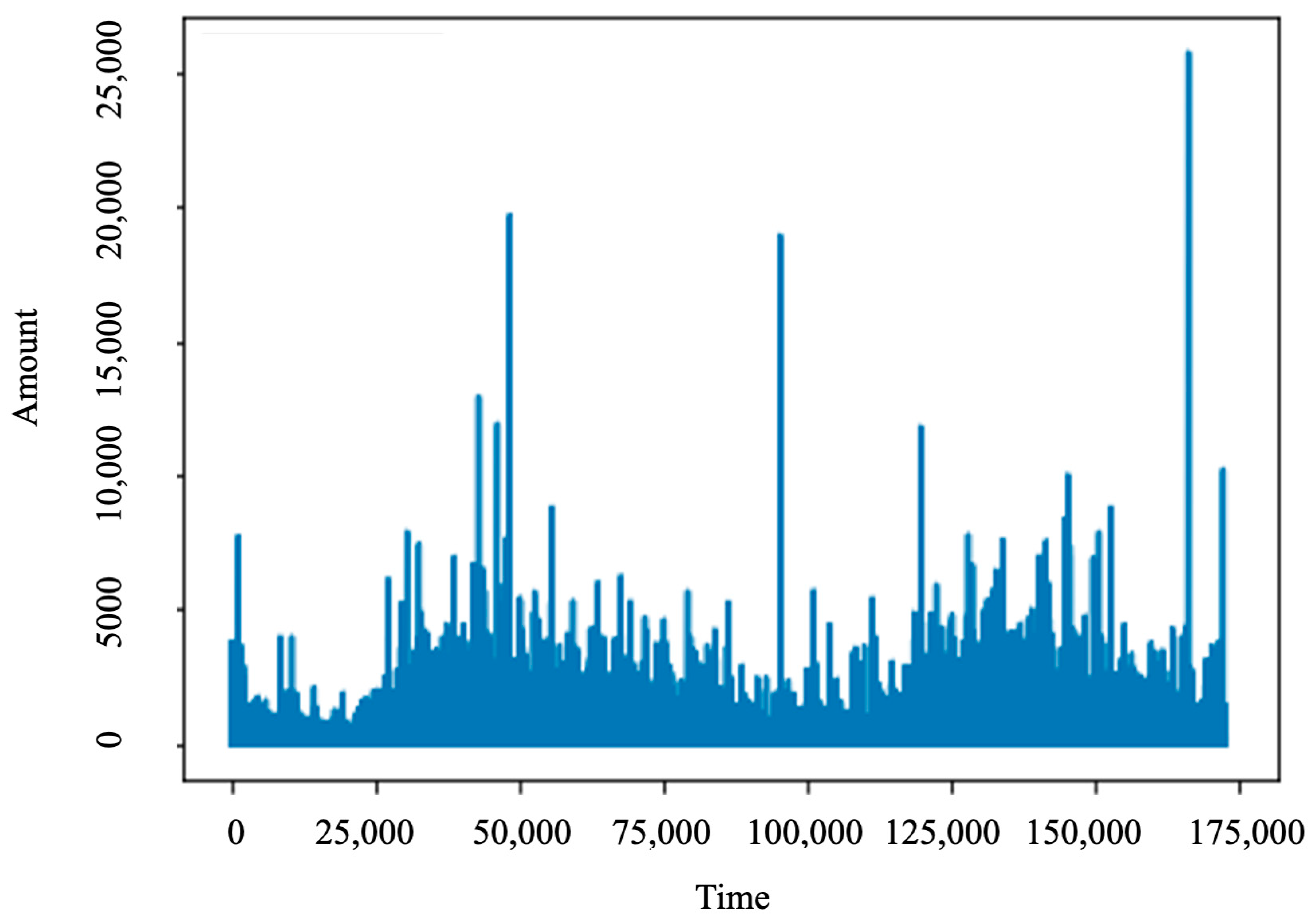
After analyzing the dataset, we recognized that the feature “Amount” has values from 0 to 25,691.16, which is illustrated in Figure 3. However, if the features are of relatively the same scale and/or close to the normal distribution, the ML algorithms will have good performances or converge faster. Therefore, standardization is used to eliminate the mean and scale to unit variance to alleviate the wide range of the feature “Amount”, so that approximately 68% of the values lie in between (−1, 1) [19]. A new feature, named “normAmount” is added to this dataset. Additionally, the “Time” and “Amount” features do not need to build models, and thus we will drop these features. We obtained the dataset of 30 features and the “Class” label.

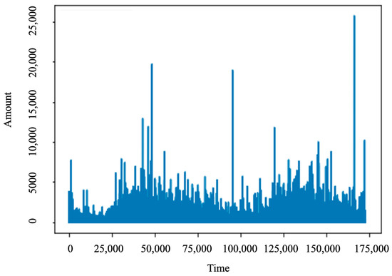
Figure 3. Plot Amount value.

3.2. Approaches for Imbalanced Datasets

In this section, we analyze different approaches to dealing with the imbalanced CCF dataset. It is obviously shown that there are two main approaches: the resampling and DRL approaches. The resampling approach is separated into two sub-approaches: the resampling approach 1 and the resampling approach 2. The difference between the two resampling approaches is the position of the resampling techniques, such as SMOTE and ADSYN. In the resampling approach 1, we resample the original CCF dataset before the train/test split, while the resampling techniques are used only for training CCF datasets in the resampling approach 2. Train/test split is divided into a ratio of 7:3. Additionally, DRL is applied directly to the original imbalanced CCF dataset. As a result, the models are evaluated comprehensively to select the best approaches for creating the CCF detection systems.

4. Resampling Techniques

There are various techniques for dealing with the imbalanced dataset [20]. These techniques are summarized and categorized into four major groups: the algorithm level, data level, cost-sensitive learning group, and ensemble-based group. First, the algorithm level technique aims at making an attempt to adapt current classifier learning algorithms to bias the learning for the minority class. Second, the purpose of the data level technique is to rebalance the classification distribution through resampling data space. Next, the cost-sensitive learning technique combines the algorithm and data level techniques to optimize the total cost errors to both classes. Finally, the ensemble-based approaches include a combination between one of the aforementioned techniques and an ensemble learning algorithm, such as the data level and cost-sensitive techniques.

Moreover, the data level methods are separated into oversampling methods, under-sampling methods, and hybrid methods. The under-sampling approaches drop instances of the majority class to make a subset of the primitive dataset. This leads to the loss of much valuable information on the original dataset. Conversely, the oversampling methods randomly duplicate instances in the minority class, so that the dataset size may increase, and this results in a rising training time for the ML models. The hybrid approach mixes both sampling methods, but these methods are quite complex.

In order to address these disadvantages, we use the SMOTE and ADASYN techniques to cope with the imbalanced dataset. This is because both techniques are popular and have demonstrated their benefits when solving imbalanced datasets in many different applications [21,22,23].

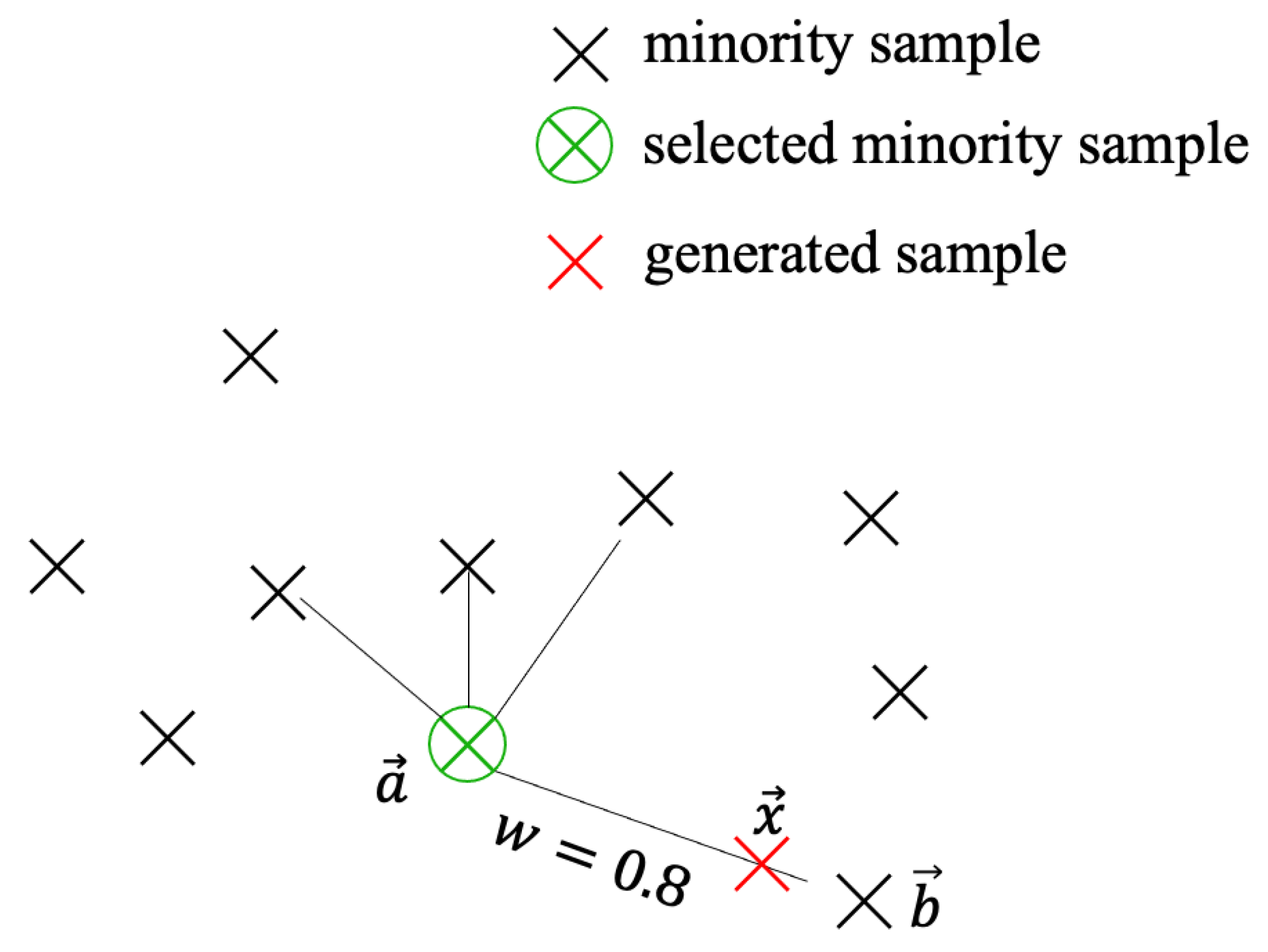
The SMOTE is one of the popular and effective oversampling techniques. The SMOTE is used to duplicate existing instances of the minority class and permitted to make a new artificial instances class based on knowledge about the neighbors that surround each sample in the minority class. The SMOTE is separated into three parts, which are known as randomizing the minority class instances, calculating k nearest neighbors for each minority class instance, and producing synthetic instances [24]. According to Figure 4 [25], this is achieved through linear interpolation of a randomly chosen minority observation and one of its observation’s neighboring minorities. To be more specific, this technique has three steps for producing a synthetic sample. The first step is to select a random minority observation $\overrightarrow{a}$. The second step is to select instance $\overrightarrow{b}$ in its k nearest minority class neighbors. The last step is to create a new sample $\overrightarrow{x}$ through random interpolation of the two samples: $\overrightarrow{x}=\overrightarrow{a}+w\times (\overrightarrow{b}-\overrightarrow{a})$, where w is denoted as a random weight in [0,1].

Figure 4. SMOTE linear interpolation of a random choose minority sample (k = 4 neighbors).

The ADASYN is a technique of improvement from the SMOTE. This technique relies on the idea of utilizing the weighted distribution to adaptively generate minority class samples: more synthetic data is produced for the minority class samples that are tougher to learn compared to the minority class samples, which are more straightforward to learn. The ADASYN technique proved its effectiveness through improving learning relevant to the distributions of data in two ways. This technique minimizes bias caused by a classification imbalance and adapts to the classification decision boundary for difficult samples [26]. The ADASYN, which illustrates input, output, and procedure, is shown in Algorithm 1.

Algorithm 1. ADSYN algorithm.

Input: Training dataset Output: Synthetic dataset from the minority class dataset Procedure:   1. The degree of balance $D_c$ is calculated as shown in (2). $$D_c=\frac{y_{min}}{y_{maj}}$$ (2) where $y_{min}$ is the number of minority class examples and $y_{maj}$ is the number of majority class examples.   2. The number of synthetic data examples created for each minority class is calculated as shown in (3). $$S= \left(y_{maj}-y_{min}\right) \times \beta$$ (3) where $\beta$ is utilized to define the desirable balance level after generating the synthetic data, and $\beta \in \left[0, 1\right]$. If $\beta =1$, a fully balanced dataset is generated after the generalization process.   3. For each example of the minority class, K nearest neighbors is calculated relied on the Euclidean distance in $n$ dimensional space, and the ratio $R_i$ is defined as shown in (4). $$R_i=\frac{{\mathsf{\Delta }}_i}{K_i}, i=1, \dots , y_{min}$$ (4) where ${\mathsf{\Delta }}_i$ is defined as the number of examples in the K nearest neighbors of the minority class, so $R_i\in \left[0, 1\right]$.   4. The normalization of $R_i$ is computed as shown in (5). $$\widehat{R_i}=\frac{R_i}{{{\displaystyle \sum }}_{i=1}^{ymin}{R}_i}$$ (5)   5. The number of synthetic data examples created for each minority example, $x_i$, is calculated as shown in (6). $$G_i=R_i\times S$$ (6) where $S$ is the total number of synthetic data examples as defined in (3).   6. Creating $G_i$ for each minority class data example follows several steps. Implementing the Loop from 1 to $G_i$ 6.1. Randomly select a minority data example, $x_{ri}$, from the K nearest neighbors for data $x_i$. 6.2. The synthetic data example is generated as shown in (7). $$s_i=x_i+ \left(x_{ri}-x_i\right) \times \lambda$$ (7) where $\lambda \in \left[0, 1\right]$ is a random number, and $\left(x_{ri}-x_i\right)$ is defined as the difference vector in a $n$ dimensional space. End Loop.

5. Machine Learning Algorithms

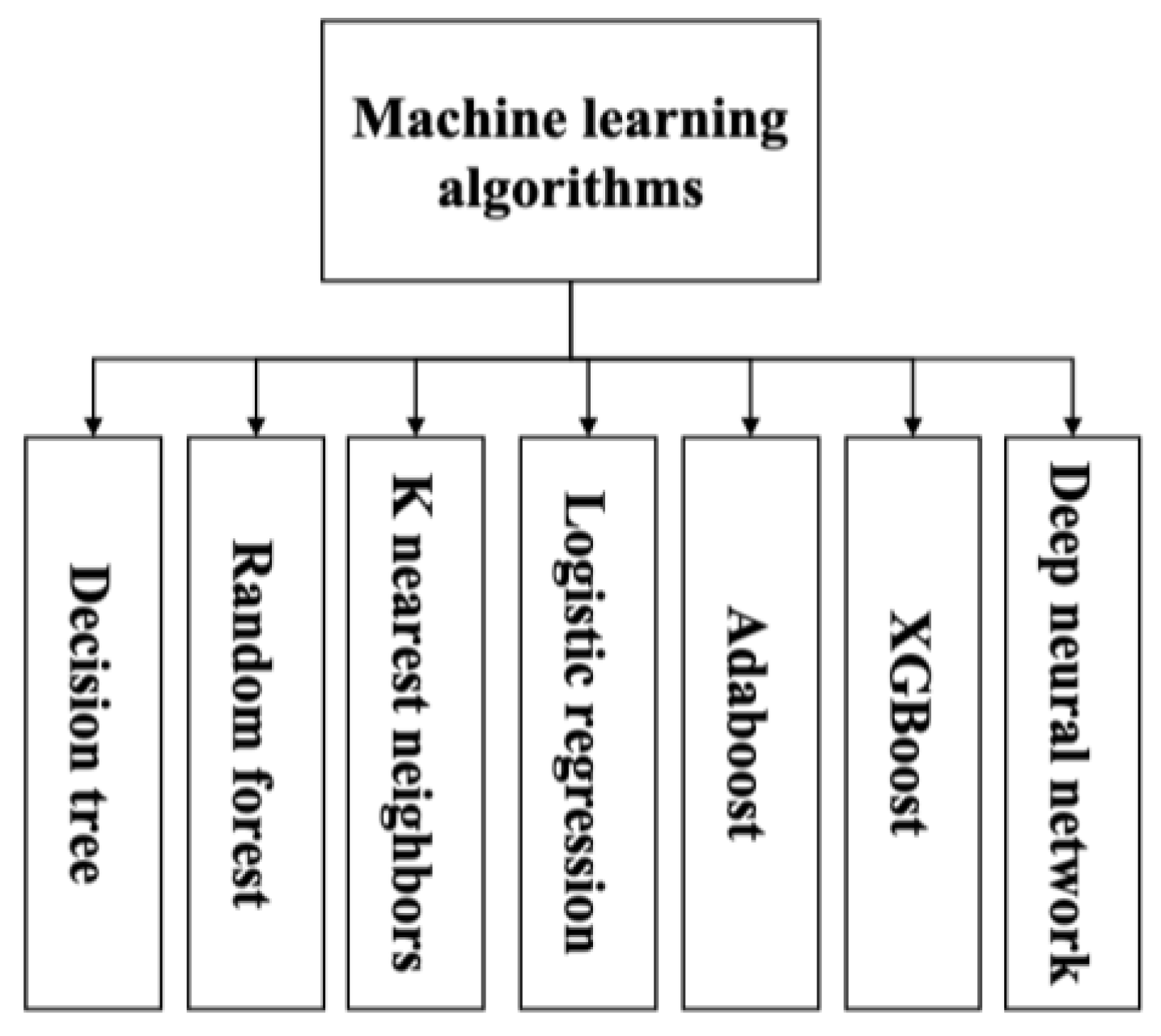
ML has been explained as lying at the intersection of computer science, engineering, and systems. It has been marked as a tool that can be applied to various problems, especially in areas that require data to be interpreted and processed [27]. ML, which is categorized as supervised machine learning, unsupervised machine learning, and reinforcement machine learning, plays an important role in solving the imbalanced dataset [28]. In this research, we select several simple but effective ML algorithms which are shown in Figure 5 to handle the imbalanced dataset. Additionally, another novel approach, named DRL, is used to deal with the imbalanced dataset, as shown in Section 6.

Figure 5. Machine learning algorithms.

5.1. K Nearest Neighbors (KNN)

The KNN algorithm, which is a non-parametric method is utilized to deal with both classification and regression problems. Although this algorithm is simple, it can outperform dramatically compared with other complex approaches. The KNN requests only k selected, a number of neighbors to be taken into account once conducting the classification. If the k value is small, the estimate of classification is susceptible to large statistical error. On the other hand, if the k value is large, this allows the distant points to contribute to the classification, resulting in the removal of several details of the class distributions. As a result, the value of k is considered to mitigate the classification error on several independent validation data or through cross-validation procedures [29,30].

5.2. Logistic Regression

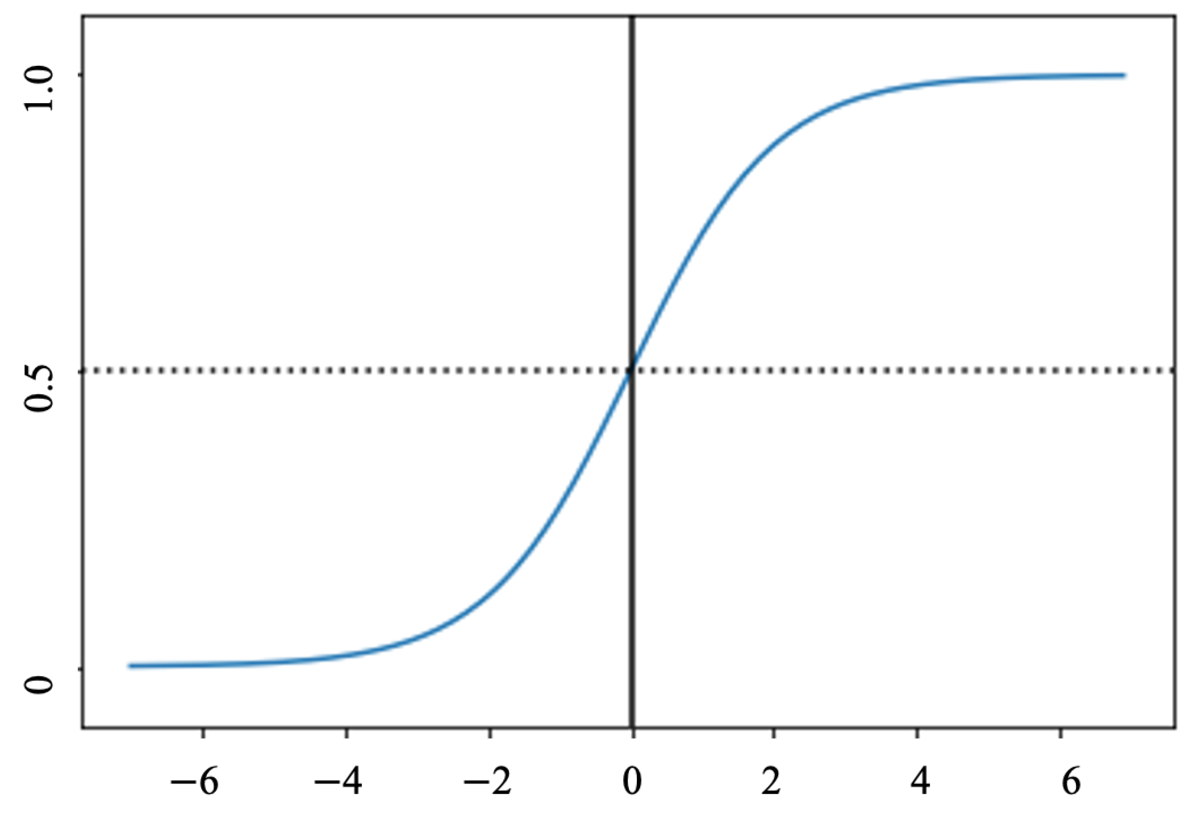
The logistic regression (LR) algorithm is one of the most prevailing approaches for binary classification. In general, the LR classifier may utilize a linear combination of more than one feature value or explanatory variable as an argument of the sigmoid function which is shown in Figure 6. The sigmoid function shown in (8) is a mathematical function that has a shape of the characteristic “S” curve. The corresponding output of the sigmoid function is a specific number that belongs to 0 and 1. The middle value is expressed as a threshold for establishing what belongs to class 1 and to class 0. To be more specific, an input that generates a result bigger than 0.5 is defined as belonging to class 1. However, the corresponding input is classified as belonging to 0 class when the output is less than 0.5 [31].

$$S\left(x\right) =\frac{1}{1+e^{-x}}=\frac{e^x}{e^x+1}=1-S\left(-x\right)$$

(8)

Figure 6. Sigmoid function.

5.3. Decision Tree

The decision tree (DT) algorithm is one of the most frequently used classifiers for classifying problems. This is mainly due to the fact that this algorithm is capable of handling complicated problems, by giving a more understandable, easier to explain representation and also because of the algorithm’s adaptability to the inference task through generating out logic classification rules. The DT encompasses nodes for checking properties, edges for branching according to values of the chosen attribute, and leaves labeling classes in which for each leaf a unique class is attached. There are two major procedures in the DT. The first procedure is to build the tree, while the second one is used for the knowledge inference, i.e., classification [32,33].

5.4. Random Forest

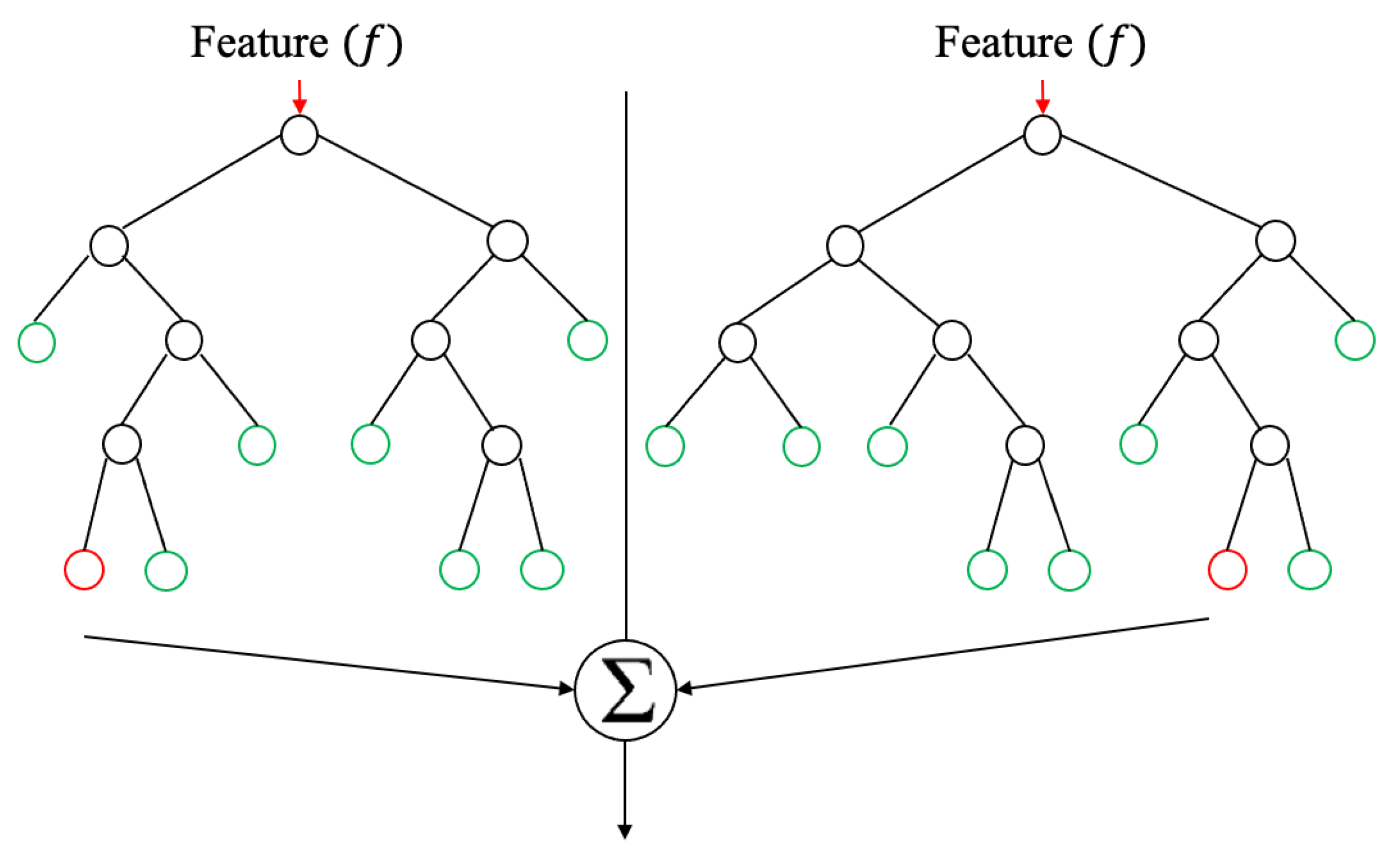
The random forest (RF) is one of the supervised learning algorithms. The big advantage of RF is that it can be used for both classification and regression. The RF is an ensemble approach that includes many decision trees. Figure 7 shows the RF with two trees [34]. This algorithm illustrates better outcomes once the number of trees in the forest is increasing and this prevents the model from overfitting. Each decision tree in the forest gives several outcomes. These outcomes are combined to achieve more accurate and stable predictions [35,36].

Figure 7. Random forest with two trees [34].

5.5. AdaBoost Algorithms

The AdaBoost algorithm is based on the Boosting idea, which is one of the most popular ensemble learning algorithms [37]. This algorithm generates classifiers through resampling data in a way that provides the richest training data for each subsequent classifier. The primary purpose of this algorithm is to train separate learning algorithms for the same training set, i.e., weak learning algorithm, and then integrate these weak learning algorithms to create a stronger, ultimate learning algorithm. In order to obtain a robust learning algorithm, we choose a weak learning algorithm and employ the same training set to continuously train the weak learning algorithm so as to enhance the weak learning algorithm’s performance. The AdaBoost algorithm consists of two weights. The first weight, named the sample weight, is present in each sample of the training set. The second weight is present in each weak learning algorithm.

AdaBoost creates a set of assumptions so that the next assumptions can concentrate on more complicated scenarios. It then integrates them by weighted majority by voting on the different categories of hypothesis prediction. The hypothesis can be produced through training a weak classifier that is employing an instance drawn from an iteratively updated distribution of the training data. This distribution update ensures that instances that are misclassified via preceding classifiers tend to be included in the training data of the subsequent classifier. Consequently, the continuous classifier training data for instances becomes increasingly difficult to classify [38].

5.6. XGBoost Algorithm

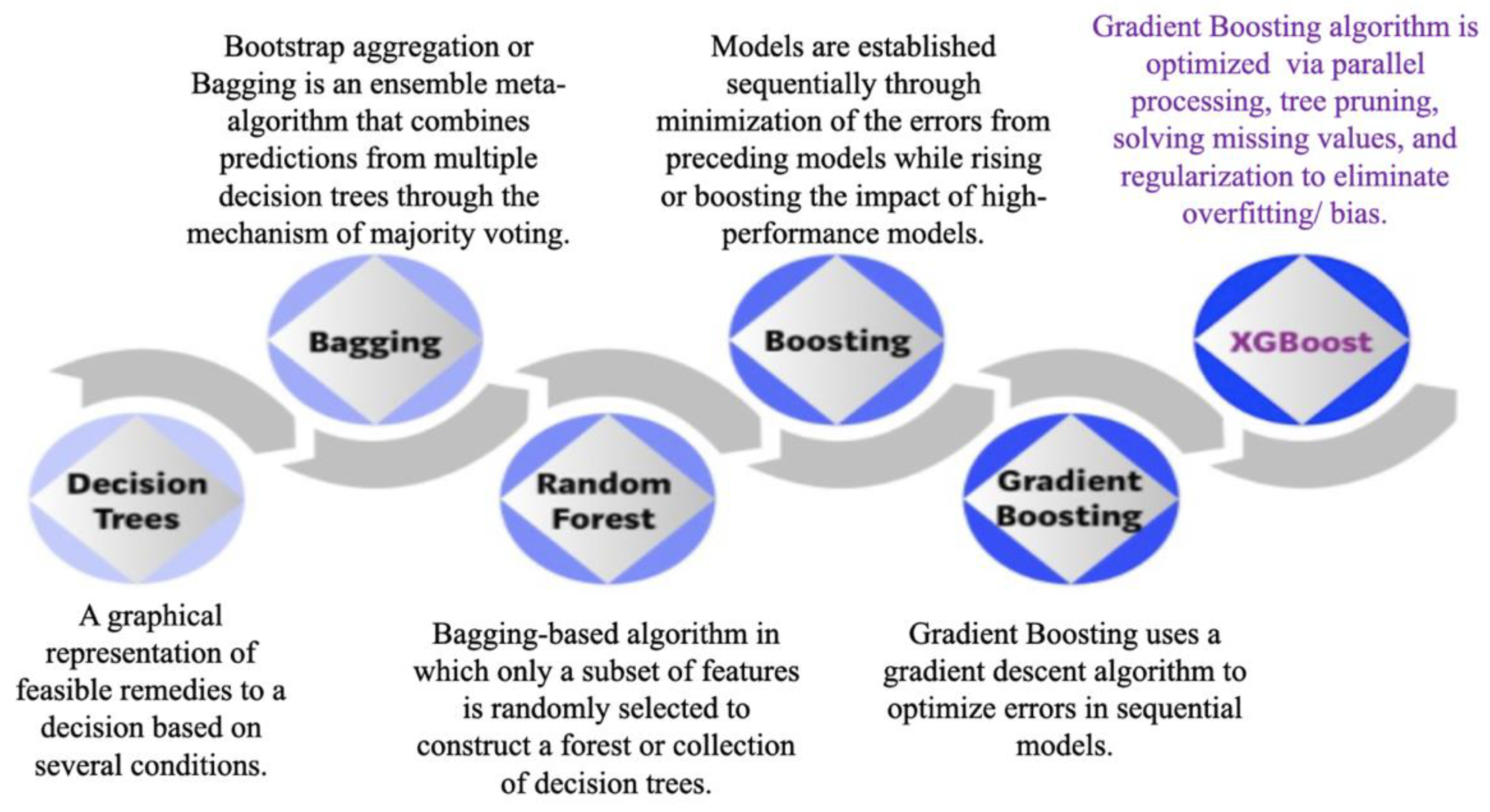
XGBoost, which has recently become one of the most popular approaches to data prediction and classification, relies on the gradient tree-boosting approach. This XGBoost algorithm has the ability to solve sparsity and avoid overfitting based on shrinkage and regularization techniques. XGBoost is designed for performance and speed, as it applies the principle of boosting weak learners by utilizing the gradient boosted decision tree implementation [39]. Figure 8 shows the evolution of XGBoost from decision trees. It is clear that the XGBoost is developed based on several previous algorithms, such as decision trees, bagging, random forest, boosting, and gradient boosting [40].

Figure 8. Evolution of XGBoost Algorithm from Decision Trees [40].

5.7. Deep Neural Network (DNN)

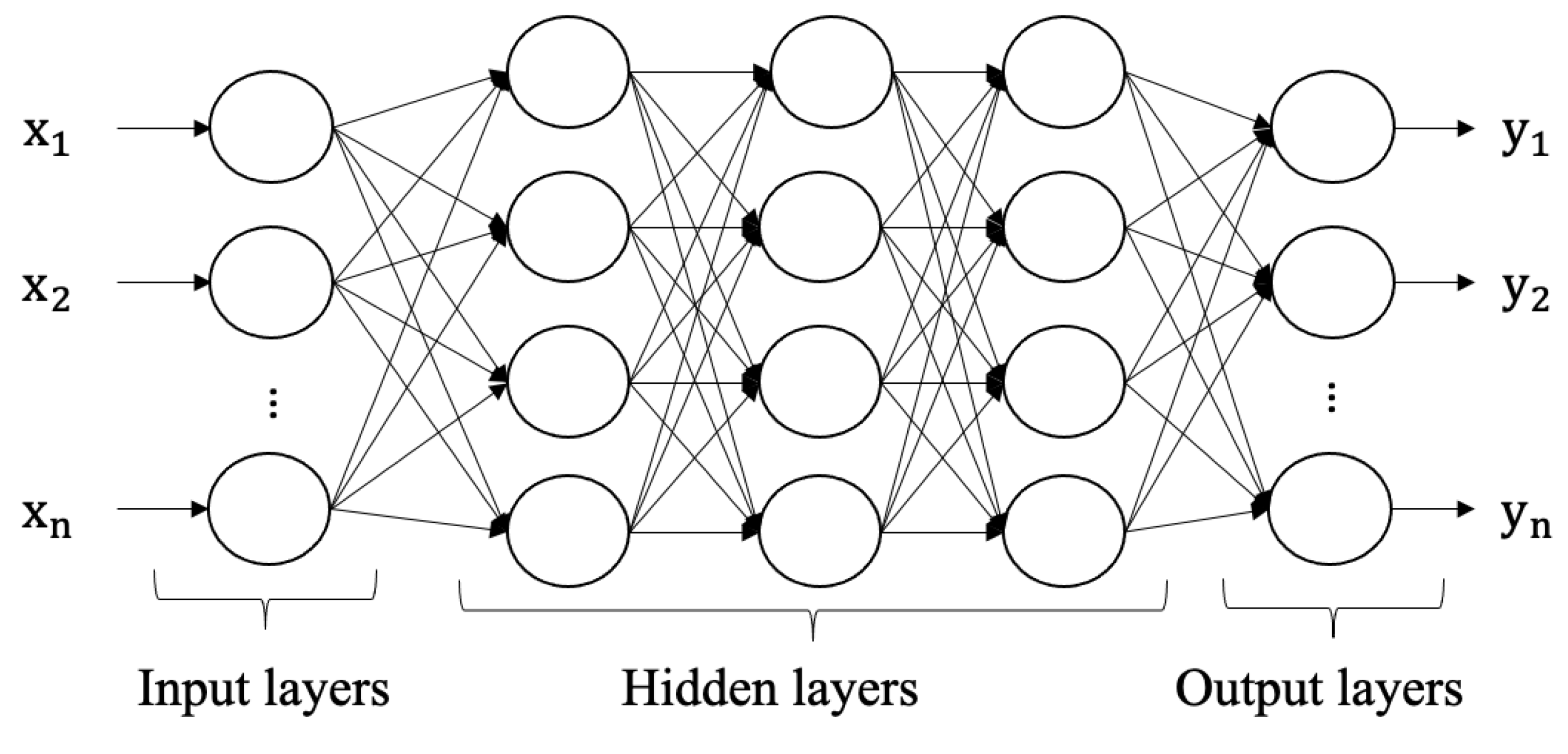
The DNN, which is an artificial neural network, includes several network layers. This approach has recently become more applicable and shows good outcomes in many different applications. The DNN classifier combines the feature extraction with classification into learning and allows for decision making. Figure 9 shows the DNN structure [41].

Figure 9. Structure of DNN.

There are several neuron layers in the DNN classifier. These neuron layers work through the activation function, named the rectified linear unit (ReLu) and expressed as (9). The output layer depends on the cost function and softmax function.

$$\mathrm{f}\left(\mathrm{x}\right) ={\mathrm{x}}^{+}=\max \left(0,\mathrm{x}\right)$$

(9)

where x is denoted as neuron input. The ReLu yields a smooth approximation to a rectifier employing an analytic function shown as (10). This is expressed as a softplus function.

$$\mathrm{f}\left(\mathrm{x}\right) =\ln \left[1+\exp \left(\mathrm{x}\right)\right]$$

(10)

When the prediction is implemented, a new raw descriptor representation, which is illustrated as (11), is extracted based on the hidden layers.

$${\mathrm{X}}_{\mathrm{l}+1}=\mathrm{H}\left({\mathrm{W}}_{\mathrm{l}}{\mathrm{X}}_{\mathrm{l}}+{\mathrm{B}}_{\mathrm{l}}\right),\mathrm{l}=1,2,\dots ,\mathrm{L}$$

(11)

where H is denoted as the activation function, $W_l$ is denoted as the weight matrix, and $B_l$ is denoted as the bias of $l^{th}$ hidden layer and these parameters are selected based on the ReLu.

5.8. Classification Metrics Performance

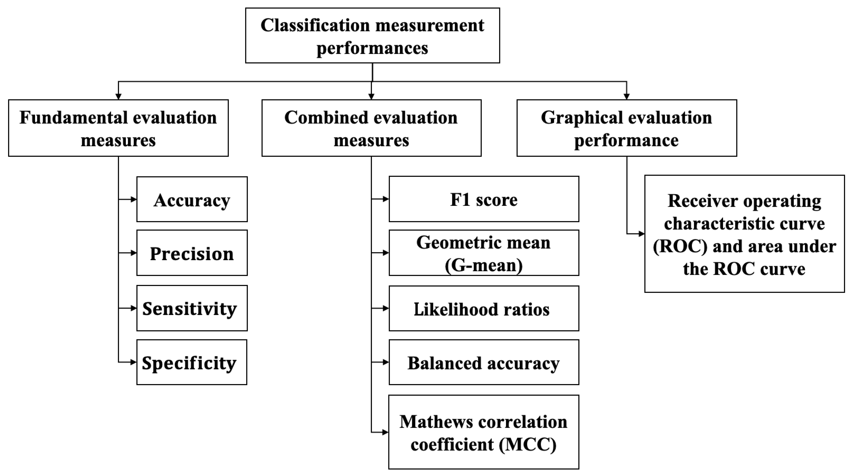
The comprehensive performance metrics for classification tasks [42,43] which are vital prerequire to establish the CCF detection systems are utilized for model evaluation of the DRL and ML algorithms. The classification metrics include three major groups which are illustrated in Figure 10. The first group is fundamental metrics, including accuracy, precision, specificity, and sensitivity. The second group is the combined metrics, such as F1 score, geometric mean (G-mean), likelihood ratios, balanced accuracy, and the Mathews correlation coefficient (MCC). The last one is the graphical plot, named the Receiver operating characteristic curve (ROC), and the area under the ROC curve (AUC).

Figure 10. Classification evaluation indexes.

5.8.1. Fundamental Evaluation Measures

In binary classification, a confusion matrix, shown in Table 2, is one of the best ways to assess the training models of the DRL and ML algorithms. The confusion matrix shows the relations between the classifier outputs and the true ones. Table 2 indicates four different combinations of predicted and actual values, explained as true positive (TP), false positive (FP), true negative (TN), and false negative (FN). In this study, samples with the presence of fraud are defined as the positive class, and samples with the absence of no-fraud are considered as the negative class. Based on the confusion matrix, accuracy, precision, sensitivity, and specificity are calculated.

Table 2. Confusion matrix.

Actual Values	Predicted Values
	Class	Negative (0)	Positive (1)
	Negative (0)	True Negative (TN)	False Positive (FP)
	Positive (1)	False Negative (FN)	True Positive (TP)

Classification accuracy is considered as one of the most popularly employed measures to the performance of classification. It is a proportion of the accurately classified samples over the total number of samples, as illustrated in (12).

$$\mathrm{Accuracy}=\frac{\left(\mathrm{TP}+\mathrm{TN}\right)}{\left(\mathrm{TP}+\mathrm{TN}+\mathrm{FP}+\mathrm{FN}\right)}$$

(12)

Positive predictive value or precision illustrates the ratio of positive samples accurately classified over the total number of positive predicted samples as shown in (13).

$$\mathrm{Precision}=\frac{\mathrm{TP}}{\left(\mathrm{TP}+\mathrm{FP}\right)}$$

(13)

Sensitivity, true positive rate, or recall illustrates the rate of positive samples that are accurately classified over the total of positive predicted samples and negative predicted samples, as indicated in (14).

$$\mathrm{Sensitivity}=\frac{\mathrm{TP}}{\left(\mathrm{TP}+\mathrm{FN}\right)}$$

(14)

Specificity is expressed as the ratio between negative samples correctly classified and the total of positive predicted samples and negative predicted samples, as shown in (15).

$$\mathrm{Specificity}=\frac{\mathrm{TN}}{\left(\mathrm{TN}+\mathrm{FP}\right)}$$

(15)

5.8.2. Combined Evaluation Metrics

Apart from the fundamental metrics, combined assessments for the binary classification are also considered as alternative approaches to assess the models, based on the DRL and ML algorithms. These assessments are straightforward but effective. This study considers several measures, such as the F1 measure, G-mean, likelihood ratios, balanced accuracy, and MCC.

The F1 measure is expressed as the harmonic mean among recall and precision, as illustrated in (16). The F1 measure has a range from 0 to 1, which means its high values reveal high classification performance.

$${\mathrm{F}}_1=\frac{2\times \left(\mathrm{Precision}\times \mathrm{Recall}\right)}{\left(\mathrm{Precision}+\mathrm{Recall}\right)}$$

(16)

The G-mean is considered as the prediction accuracy outcome for both sensitivity and specificity, as illustrated in (17).

$$\mathrm{G}=\sqrt{\mathrm{Sensitivity}\times \mathrm{Specificity}}$$

(17)

The Likelihood ratios are separated as a positive likelihood ratio and a negative likelihood ratio. The positive likelihood ratio is defined as the ratio sensitivity over one minus specificity, as shown in (18).

$$\mathrm{L}=\frac{\mathrm{Sensitivity}}{1-\mathrm{Specificity}}$$

(18)

Conversely, the negative likelihood ratio is expressed in (19) as the ratio between one minus sensitivity and specificity.

$$\mathsf{\lambda }=\frac{1-\mathrm{Sensitivity}}{\mathrm{Specificity}}$$

(19)

Based on the definition of the negative likelihood ratio and the positive likelihood ratio, a lower negative likelihood and a higher positive likelihood ratio will have correspondingly better performances on negative and positive classes. The threshold of positive likelihood is shown in Table 3.

Table 3. Interpretation of Thresholds of Positive Likelihood.

L Value	Contribution of Model
>10	Good
5–10	Fair
1–5	Poor
1	Negligible

The balanced accuracy represents the average of sensitivity and specificity, as shown in (20).

$$\mathrm{Balanced}\mathrm{Accuracy}=\frac{\mathrm{Sensitivity}+\mathrm{Specificity}}{2}$$

(20)

MCC is not affected by the imbalanced dataset problem. MCC illustrated in (21) is defined as a contingency matrix approach of computing the Pearson product-moment correlation coefficient between the predicted and actual values.

$$\mathrm{MCC}=\frac{\mathrm{TP}\times \mathrm{TN}-\mathrm{FP}\times \mathrm{FN}}{\sqrt{\left(\mathrm{TP}+\mathrm{FP}\right)\left(\mathrm{TP}+\mathrm{FN}\right)\left(\mathrm{TN}+\mathrm{FP}\right)\left(\mathrm{TN}+\mathrm{FN}\right)}}$$

(21)

5.8.3. Graphical Evaluation Performance

The ROC curve, which is a graphical evaluation, describes the diagnostic capability of a binary classifier system since its taxonomy threshold is different. The ROC curve is established by plotting the ratio of true positive versus false positive rates. The AUC measures the whole two-dimensional area under the whole ROC curve. The AUC can assess models in terms of overall performance, and thus it is more considered in its model evaluation. The suggestion of the following scale for AUC value interpretation is shown in Table 4.

Table 4. AUC Performance.

AUC Value	Performance of Model
0.9–1.0	Excellent
0.8–0.9	Very good
0.7–0.8	Good
0.6–0.7	Fair
0.5–0.6	Poor

6. Deep Reinforcement Learning for Imbalanced Classification

6.1. Imbalanced Classification Markov Decision Process

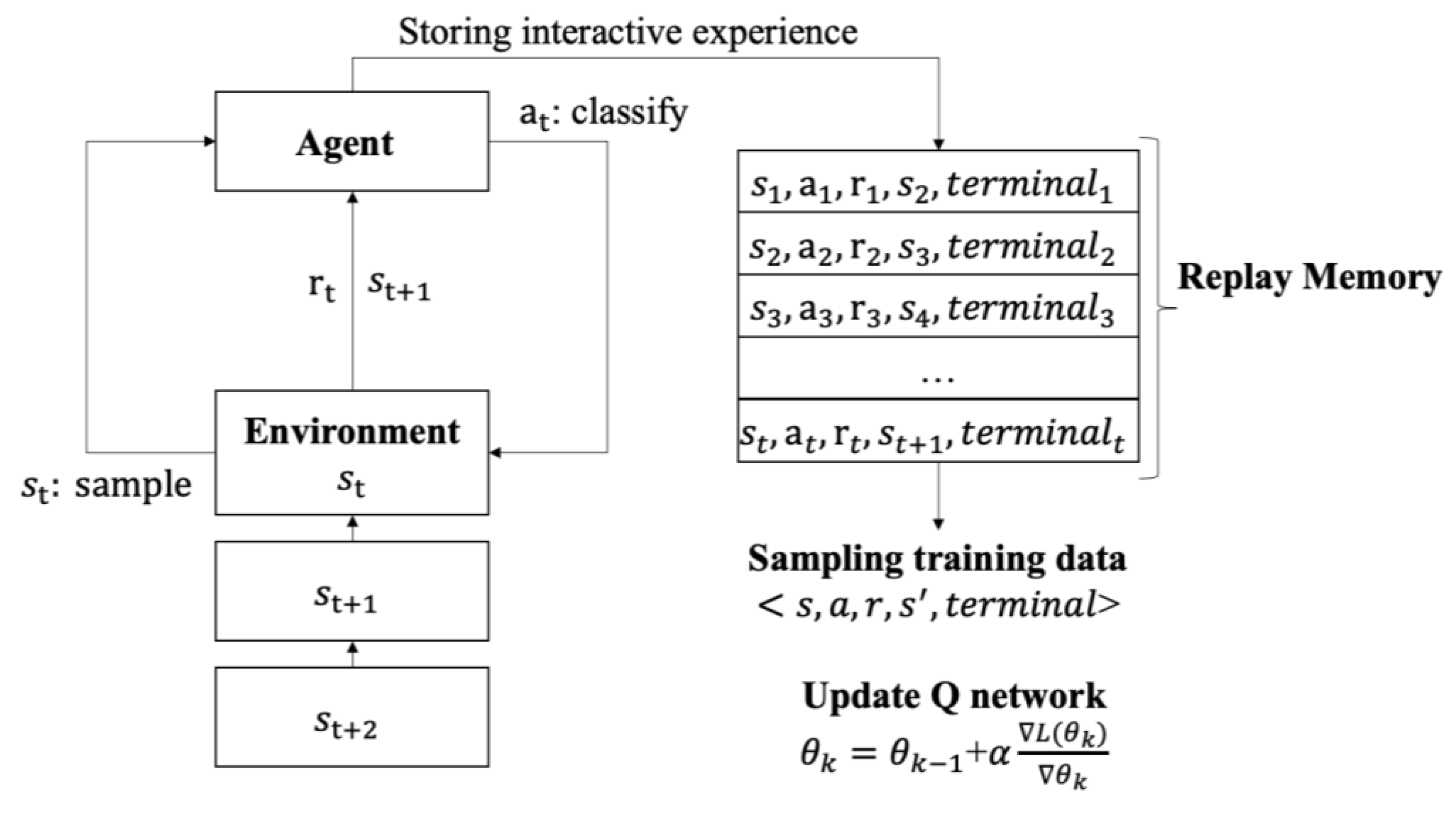
Reinforcement learning (RL) algorithms incorporated deep learning (DL) in order to defeat world champions at the Go game and human experts who perform various Atari video games. We express the problem of classification as a guessing game. As shown in Figure 11, the agent receives a sample $s_t$ at each time step and classifies what the sample is, and thus the environment returns it an immediate reward $r_t$ and provides the next sample $s_{t+1}$. If the agent accurately classifies the sample category, the agent receives a positive reward through the environment. If the agent does not accurately classify the sample category, the agent receives a negative reward through the environment. The agent may accurately guess the samples as much as possible to accumulate the maximum rewards. In order to obtain this accumulation, the agent learns an optimal behavior from its interaction with the environment [4].

Figure 11. ICMDP process.

The Imbalanced Classification Markov Decision Process (ICMDP) framework is formalized in this paper. The purpose of the ICMDP framework is to decompose the classification task of the imbalanced data into a sequential decision-making problem. For instance, the imbalanced training dataset is $D=\left\{\left(x_1,l_1\right), \left(x_2,l_2\right), \dots , \left(x_n,l_n\right) \right\}$, where $x_i$ is expressed as the $i^{th}$ sample, and $l_i$ is defined as the label of the $i^{th}$ sample. Based on the ICMDP, we propose to train a classifier as an agent with many components, as follows.

State$\mathit{S}$: The state is identified by the training sample. The agent receives the first sample $x_1$ as an initial state $s_1$ at the beginning of training. The state $s_t$ of the environment at each time step corresponds to the sample $x_t$. When the new episode launches, the order of samples in the training dataset is shuffled in the environment.

Action$\mathit{A}$: The action relates to the training dataset label. The action which is taken by the agent aims at predicting the label of the class. In case of the binary classification, the action is defined as $A=\{0,1$} where 0 shows the minority class and 1 illustrates the majority class.

Reward$\mathit{R}$: The reward $r_t$ is the response from the environment to measure the success or failure of the agent-based actions. In the imbalanced dataset, we want to direct the agent to learn the policy of optimal classification, so the absolute reward value of sample in the majority class is lower than that in the minority class. It means that if the agent correctly or incorrectly recognizes the minority class sample, the environment will feedback a larger reward or punishment to the agent, respectively.

Transition probability$\mathit{P}$: The transition probability $P(s_{t+1}|s_t,a_t)$ is deterministic in the ICMDP. Based on the order of samples in the training dataset, the agent can move from the current state $s_t$ to the subsequent state $s_{t+1}$.

Discount factor$\mathbf{\gamma }$: The discount factor is defined as $\gamma$, which belongs to $\left[0,1\right]$. The discount factor aims at balancing the immediate and future rewards.

Episode: The episode is a transition trajectory, which is a sequence of states and actions influencing those states. If all samples in the training dataset are classified or the agent misclassifies the sample from the minority class, an episode will complete.

Policy${\mathbf{\pi }}_{\mathbf{\theta }}$: The policy ${\pi }_{\theta }$ is defined as a mapping function $\pi$: $\mathit{S} \to \mathit{A}$, where ${\pi }_{\theta }$($s_t$) is the action which is performed by the agent in state $s_t$. In the ICMDP, the policy ${\pi }_{\theta }$ is expressed as a classifier with the parameter $\theta$.

According to the aforementioned notations and definitions, the problem of imbalanced classification is considered as to search for the optimal classification policy ${\pi }^{*}$: $\mathit{S} \to \mathit{A}$. This policy can maximize the cumulative rewards in the ICMDP.

6.2. Imbalanced Data Classification Reward Function

The samples of minority class are tough to accurately identify in the imbalanced datasets. In order to better detect the samples of the minority class, the algorithm is more sensitive to the minority class. A big reward or penalty will be returned to the agent when it encounters the minority sample. The reward function is expressed, as shown in (22).

$$R\left(s_t,a_t,l_t\right)=\left\{\begin{array}{c}+1 a_t=l_{t }and s_t\in D_{min}\\ -1 a_t\ne l_{t }and s_t\in D_{min}\\ \lambda a_t=l_{t }and s_t\in D_{maj}\\ -\lambda a_t\ne l_{t }and s_t\in D_{maj}\end{array}\right.$$

(22)

where $\lambda \in \left[0, 1\right]$ is a trade-off parameter and is used to regulate the importance of the majority class, $D_{min}$ is the sample set of the minority class, $D_{maj}$ is the sample set of the majority class, $l_t$ is expressed as the class label of the sample in the state $s_t$. If the agent inaccurately or accurately classifies the sample of the minority class, the value of the reward is $-1$ or $1$, respectively. Similarly, if the agent inaccurately or accurately classifies the sample of the majority class, the value of the reward is $-\lambda$ or $\lambda$, respectively. The reward function value is the predicted cost of the agent. If the training dataset is imbalanced ($\lambda <1$), the prediction cost values of the majority class are lower than that of the minority class. By contrast, the values of prediction cost are the same for both classes when the training dataset is balanced ($\lambda =1$).

6.3. Deep Q-Network Based Imbalanced Classification Algorithm

6.3.1. Deep Q-Learning for ICMDP Subsection

According to ICMDP, the classification policy $\pi$, shown in (23), is considered as a function. This function receives a sample and returns the probabilities of both labels.

$$\pi \left(a|s\right) =P(a_t=a|s_t=s)$$

(23)

The classifier agent aims at accurately identifying as many training data samples as possible. Since the classifier agent obtains a positive reward for correctly identifying the sample, it then accomplishes its objective through maximization of the cumulative rewards $g_t$, shown in (24).

$$g_t={\displaystyle \sum }_{k=0}^{\infty }{\gamma }^k{r}_{t+k}$$

(24)

In the RL, the function which is the Q function is used to calculate the quality of the association between the state and the action. The Q function is shown in (25).

$$Q^{\pi }\left(s,a\right) =E_{\pi }[g_t|s_t=s, a_t=a]$$

(25)

Based on the Bellman equation [36], the Q function is defined in (26).

$$Q^{\pi }\left(s,a\right) =E_{\pi }[r_t+\gamma Q^{\pi }\left(s_{t+1},a_{t+1}\right)|s_t=s, a_t=a]$$

(26)

In the ICMDP, through resolving the optimal $Q^{*}$ function, the classifier agent maximizes the cumulative rewards. The optimal classification policy ${\pi }^{*}$ is defined as the greedy policy under the optimal $Q^{*}$ function shown in (27).

$${\pi }^{*}\left(a|s\right) = \left\{\begin{array}{c}\begin{array}{cc}1,& if a=\arg ma{x}_a{Q}^{*}\left(s,a\right)\end{array}\\ \begin{array}{cc}0 & else\end{array}\end{array}\right.$$

(27)

The optimal $Q^{*}$ function, which is shown in (28), is obtained through substituting (27) into (26).

$$Q^{*}\left(s,a\right) =E_{\pi }[r_t+\gamma \underset{a}{\underbrace{max}}{Q}^{*}\left(s_{t+1},a_{t+1}\right)|s_t=s, a_t=a]$$

(28)

The Q functions are written down through a table in the low-dimensional finite state space. By contrast, the Q functions are solved based on the deep Q-learning algorithm in high-dimensional continuous state space. In the deep Q-learning algorithm, the interaction data $\left(s,a,r,s^{\prime }\right)$, which is achieved from (28), are accumulated in the experience replay memory M. The agent is random sampling a mini batch of transitions B from M and implements a gradient descent step on the deep Q network which relies on the loss function, as illustrated in (29).

$$L\left({\theta }_k\right) ={\displaystyle \sum }_{\left(s, a, r, s^{\prime }\right)\in B}{\left(y-Q\left(s,a;{\theta }_k\right)\right)}^2$$

(29)

where y is defined as the target estimation of the Q function as shown in (30).

$$y = \left\{\begin{array}{c}\begin{array}{cc}r, & ternimal=True\end{array}\\ \begin{array}{cc}r+\gamma ma{x}_{a^{\prime }}Q\left(s^{\prime },a^{\prime };{\theta }_{k-1}\right),& terminal=False\end{array}\end{array}\right.$$

(30)

where $s^{\prime }$ is denoted as the subsequent state of s, and $a^{\prime }$ is the action which is performed by the agent in the state $s^{\prime }$.

The derivative of the loss function (29) with θ is shown in (31).

$$\frac{\nabla L\left({\theta }_k\right)}{\nabla {\theta }_k}=-2 {\displaystyle \sum }_{\left(s,a,r,s^{\prime }\right)\in B}\left(y-Q\left(s,a;{\theta }_k\right)\right)\frac{\nabla Q\left(s,a;{\theta }_k\right)}{\nabla {\theta }_k}$$

(31)

The optimal $Q^{*}$ function is obtained through minimization of the loss function (29). The greedy policy (27) under the optimal $Q^{*}$ function receives the maximum cumulative rewards. Therefore, the optimal classification policy ${\pi }^{*}$: $S \to A$is accomplished.

6.3.2. Influence of Reward Function

In the imbalanced dataset, the trained Q network is biased against the majority class. Nevertheless, owing to the reward function mentioned in (22), different rewards are assigned for different classes and ultimately different classes which have the same influence on the Q network are made samples.

It is assumed that $s^{+}$ and $s^{-}$ are defined as the positive and negative samples, respectively and $y^{+}$ and $y^{-}$ are the target Q values. Based on (22) and (30), the target Q values are shown in (32) and (33).

$$y^{+}=\left\{\begin{array}{c}\begin{array}{cc}{\left(-1\right)}^{1-I\left(a=l\right)} & terminal=True\end{array}\\ \begin{array}{cc}{\left(-1\right)}^{1-I\left(a=l\right)}+\gamma ma{x}_{a^{\prime }}Q\left(s^{\prime },a^{\prime }\right),& terminal=False\end{array}\end{array}\right.$$

(32)

$$y^{-}=\left\{\begin{array}{c}\begin{array}{cc}{\left(-1\right)}^{1-I\left(a=l\right)}\lambda , & terminal=True\end{array}\\ \begin{array}{cc}{\left(-1\right)}^{1-I\left(a=l\right)}\lambda +\gamma ma{x}_{a^{\prime }}Q\left(s^{\prime },a^{\prime }\right),& terminal=False\end{array}\end{array}\right.$$

(33)

where $I\left(x\right)$ is denoted as an indicator function.

According to loss function $L\left({\theta }_k\right)$, the sum of negative class loss function $L_{-}\left({\theta }_k\right)$ and positive class loss function $L_{+}\left({\theta }_k\right)$ are formed, and their derivatives are expressed in (34) and (35).

$$\frac{\nabla L_{+}\left({\theta }_k\right)}{\nabla {\theta }_k}=-2{{\displaystyle \sum }}_{i=1}^{D_{min}}(y_i^{+}-Q\left(s_i^{+},a_i;{\theta }_k\right))\frac{\nabla Q\left(s_i^{+},a_i;{\theta }_k\right)}{\nabla {\theta }_k}$$

(34)

$$\frac{\nabla L_{-}\left({\theta }_k\right)}{\nabla {\theta }_k}=-2{{\displaystyle \sum }}_{j=1}^{D_{maj}}(y_i^{-}-Q\left(s_j^{-},a_j;{\theta }_k\right))\frac{\nabla Q\left(s_j^{-},a_j;{\theta }_k\right)}{\nabla {\theta }_k}$$

(35)

where $D_{min}$ and $D_{maj}$ are total positive and negative sample sets, respectively.

We replace (32) into (34), (33) into (35) and add the derivative of $L_{+}\left({\theta }_k\right)$) and $L_{-}\left({\theta }_k\right)$, and we then obtain (36).

$$\begin{gathered} \frac{\nabla L\left({\theta }_k\right)}{\nabla {\theta }_k}=-2{\displaystyle \sum }_{m=1}^{D_{min}+D_{maj}}\left((1-t_m\right)\gamma \underset{a_m^{\prime }}{\underbrace{max}}Q\left(s_m^{\prime };a_m^{\prime };{\theta }_{k-1}\right) \\ -Q\left(s_m,a_m;{\theta }_k\right))\frac{\nabla Q\left(s_m,a_m;{\theta }_k\right)}{\nabla {\theta }_k} \\ -2{{\displaystyle \sum }}_{i=1}^{D_{min}}{\left(-1\right)}^{1-I\left(a_i=l_i\right)} \frac{\nabla Q\left(s_i,a_i;{\theta }_k\right)}{\nabla {\theta }_k} \\ -2\lambda {{\displaystyle \sum }}_{i=1}^{D_{min}}{\left(-1\right)}^{1-I\left(a_j=l_j\right)} \frac{\nabla Q\left(s_j,a_j;{\theta }_k\right)}{\nabla {\theta }_k} \end{gathered}$$

(36)

where $t_m=0$ if $terminal=False$, and $t_m=1$ if $terminal=True$.

Based on (36), the second part indicates the minority class, and the third part illustrates the majority class. In the case of the imbalanced dataset, if the value of $\lambda$ is equal to 1, the immediate rewards of the two classes are identical. The value of the second part is smaller than that of the third part, as the number of samples in the minority class is less than that in the majority class. Therefore, the model is biased to the majority class. If the $\lambda$ value is less than 1, $\lambda$ will mitigate the immediate rewards of negative samples and will weaken their influences on the loss function of the Q network.

7. Results

In order to provide various solutions to deal with the imbalanced CCF dataset, all results related to the ML algorithms and the DRL approach based on the imbalanced CCF dataset are indicated in this section. Section 7.1 describes the outcomes of models based on the seven ML algorithms for the imbalanced CCF datasets. In this section, we indicate the paradox accuracy of the seven ML models of CCF detection. Next, the problem of paradox accuracy is solved in Section 7.2 and Section 7.3. These two sections illustrate the results of seven ML models of CCF detection based on the resampling approach 1 and resampling approach 2. The performance comparison between the two sampling approaches is also indicated in these sections. Finally, Section 7.4 shows the outcomes of the model, based on the DRL for the imbalanced CCF dataset.

7.1. Results of Machine Learning Models Based on Imbalanced CCF Dataset

The performance of seven ML algorithms on the imbalanced CCF dataset is represented in this section. The confusion matrices, including true positive, false positive, true negative, and false negative rates, of RF, KNN, DT, LR, AdaBoost, XGBoost, and DNN classifiers obtained on the imbalanced CCF dataset are shown in Table 5.

Table 5. TP, FP, TN, FN rates of machine learning algorithms on imbalanced dataset.

Rate	RF	KNN	DT	LR	AdaBoost	XGBoost	DNN
TP	113	106	111	91	101	115	119
FP	6	7	25	12	17	8	24
TN	85,290	85,289	85,271	85,284	85,279	85,288	85,272
FN	1	41	36	1	46	32	32

The accuracies of the mentioned ML models on the imbalanced CCF dataset are indicated in Table 6. Based on Table 6, the accuracies values of the mentioned ML models of CCF detection are extremely high. The aforementioned confusion matrices show that the TP samples are much less than TN samples. However, in order to establish a reliable CCF detection system, positive samples should be detected more frequently than negative ones. We, therefore, need to improve these models despite their high accuracies.

Table 6. Accuracies of the ML models on imbalanced dataset.

Algorithms	RF	KNN	DT	LR	AdaBoost	XGBoost	DNN
Accuracy	99.95%	99.94%	99.91%	99.92%	99.92%	99.95%	99.94%

7.2. Results of Machine Learning Models Based on Resampling on Approach 1

As indicated in Section 7.1, the ML models on the imbalanced CCF dataset do not show good performance in terms of detecting the CCF activities, and thus we need to resample this imbalanced CCF dataset to the balanced CCF dataset, and then apply the ML methods to accomplish better models for CCF detection. According to the resampling approach 1, the performances of seven ML approaches based on SMOTE and ADASYN techniques are evaluated for the prediction of CCF using 30 features, as discussed in Section 3. The confusion matrices of RF, KNN, DT, and LR, and the AdaBoost, XGBoost, and DNN algorithms, based on the resampled CCF dataset, are accomplished to identify the TN, FN, FP, and TP rates. The rates of the machine learning algorithms with SMOTE are illustrated in Table 7. The rates of the machine learning algorithms with ADASYN are represented in Table 8. It is clearly shown that the TP samples are greater than the TN sample based on the ML algorithms on the resampling datasets. This is the first step in demonstrating the effectiveness of applying two resampling techniques to the CCF dataset.

Table 7. TP, FP, TN, FN rates of machine learning algorithms with SMOTE based on resampling approach 1.

Rate	RF with SMOTE	KNN with SMOTE	DT with SMOTE	LR with SMOTE	AdaBoost with SMOTE	XGBoost with SMOTE	DNN with SMOTE
TP	85,427	85,427	85,314	78,171	82,219	85,496	85,238
FP	19	209	270	2117	1466	53	262
TN	85,143	84,953	84,892	83,045	83,663	85,040	85,020
FN	0	0	113	7256	3241	0	69

Table 8. TP, FP, TN, FN rates of machine learning algorithms with ADASYN based on resampling approach 1.

Rate	RF with ADASYN	KNN with ADASYN	DT with ADASYN	LR with ADASYN	AdaBoost with ADASYN	XGBoost with ADASYN	DNN with ADASYN
TP	85,428	85,429	85,366	73,864	71,308	85,205	85,276
FP	30	179	218	7194	1475	111	503
TN	85,128	84,979	84,940	77,244	84,028	85,271	84,778
FN	1	0	63	11,565	13,776	0	30

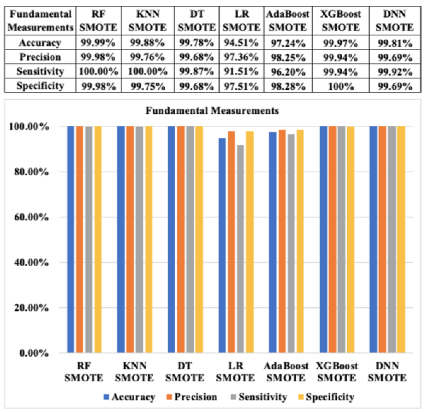
Additionally, the fundamental classification performance metrics of seven ML algorithms for CCF detection with SMOTE and ADASYN based on approach 1 are revealed in Figure 12 and Figure 13, respectively. According to Figure 12, the accuracies of the aforementioned algorithms with the resampled CCF datasets are almost similar (above 99%), except the LR algorithm, which has an accuracy of approximately 94.51% based on SMOTE. The precision of the seven ML algorithms also indicates positive outcomes with the highest value of 99.98% for RF with SMOTE. Similarly, the specificity of all of the mentioned algorithms shows very high results (above 99%), except for the LR algorithms, which have a specificity result of approximately 97.51% based on SMOTE. Furthermore, the sensitivity reveals extremely good outcomes, approximately 100% in terms of RF and KNN with the SMOTE technique.

Figure 12. Fundamental classification performance measurements of ML algorithms with SMOTE based on resampling approach 1.

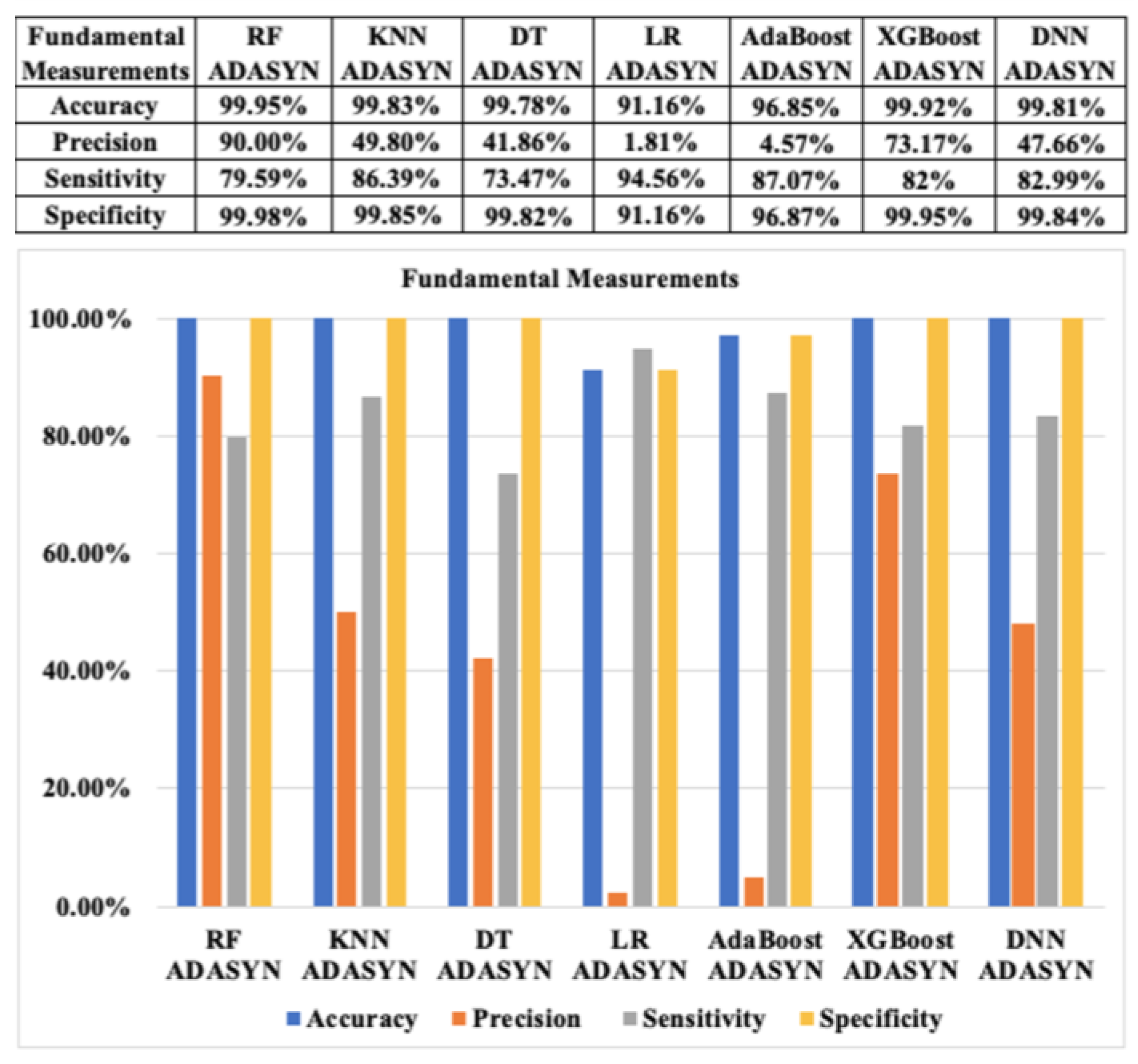
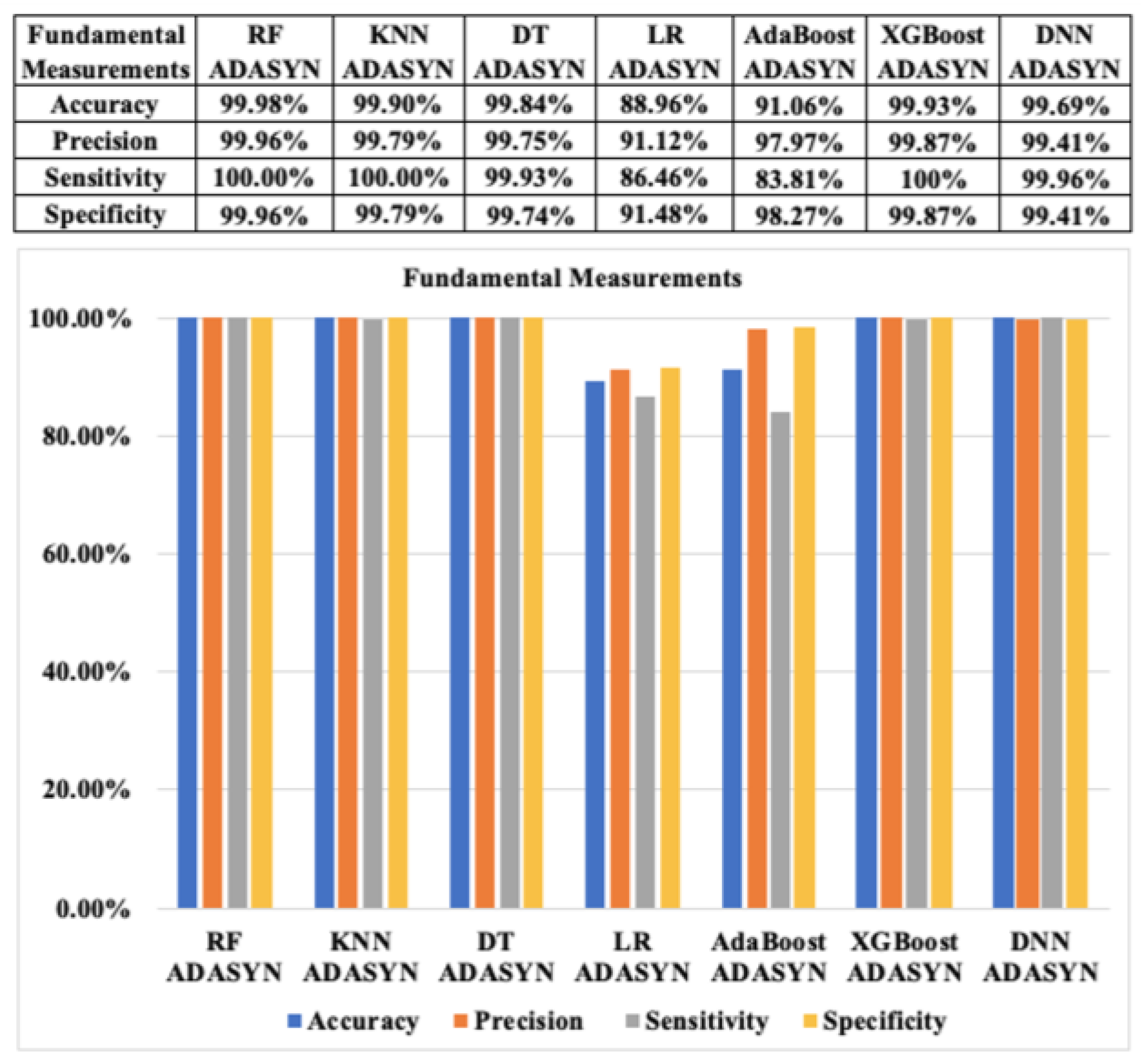
Figure 13. Fundamental classification performance measurements of ML algorithms with ADASYN based on resampling approach 1.

Based on Figure 13, the accuracies of the seven ML classifiers for CCF detection with ADASYN are also very good, except for the LR algorithm, which is approximately 88.96%. This is similar to the case of SMOTE, and the values of other metrics, such as precision, sensitivity, and specificity of the ML algorithms with ADASYN, show very positive outcomes. However, the sensitivity results of LR and AdaBoost based on ADASYN are quite low compared with other classifiers, at only approximately 86.46% and 83.81%, respectively.

In general, we also can observe that the results of the seven ML methods for CCF detection based on SMOTE and ADASYN are quite similar in each ML approach. The fundamental metrics illustrate excellent outcomes of the seven ML approaches with the resampling CCF dataset. The fundamental classification metrics show the results of not only the accuracy value, but also other values, as mentioned, to evaluate the ML models of CCF detection more comprehensively. However, the performance of LR and AdaBoost classifiers for CCF detection based on both SMOTE ADASYN have the lowest results regarding all fundamental metrics among seven classifiers.

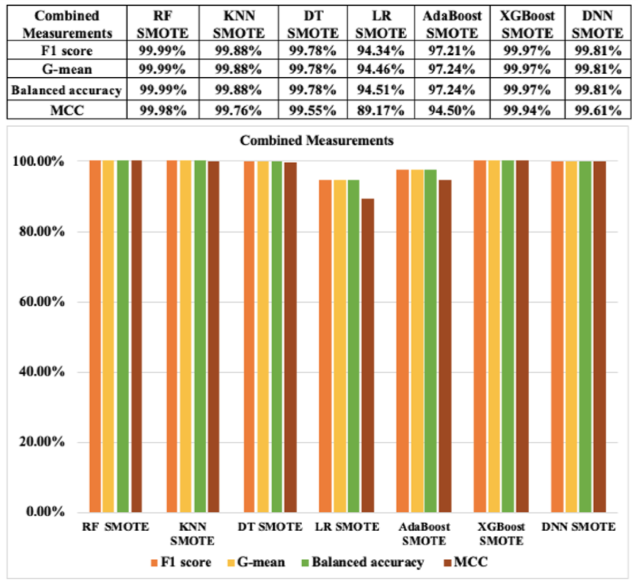
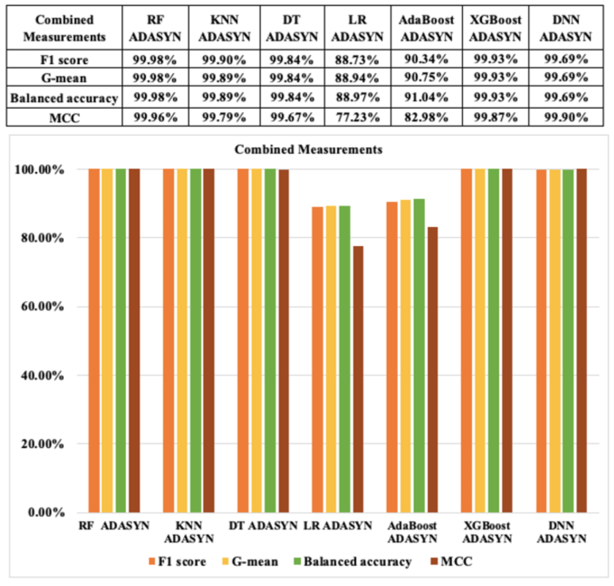
Next, in terms of combined metrics based on the resampling approach 1, indexes, such as the F1 score, G-mean, balanced accuracy, and MCC, of the seven ML algorithms for CCF detection which relied on SMOTE and ADASYN are displayed in Figure 14 and Figure 15, respectively. Overall, the results of the combined metrics of the ML models based on resampling CCF dataset are also very high. The results of RF, KNN, DT, XGBoost, and DNN classifiers for CCF with SMOTE and ADASYN are also similar, above 99%. However, the outcomes of LR and AdaBoost with SMOTE and ADASYN show relatively low results, particularly the result of only 77.23% of the MCC index in the case of ADASYN. We see that LR with ADASYN has the lowest results of all indexes in the combined metrics. However, RF and DNN with SMOTE and ADASYN results are almost similar and show the highest values for all these indexes to detect CCF.

Figure 14. Combined classification performance measurements with SMOTE based on resampling approach 1.

Figure 15. Combined classification performance measurements with ADASYN based on resampling approach 1.

Based on the resampling approach 1, the positive likelihood ratios of the seven ML models of CCF detection that were computed are shown in Table 9. Based on Table 3, it is clear that all of the model contributions are good. However, there is a dramatic difference between the outcomes of these models. The results of RF are very high, at about 4482.21, while LR shows very low results, at only 10.15.

Table 9. Positive Likelihood Ratio based on resampling approach 1.

ML Algorithms		Positive Likelihood Ratio	Model Contribution
RF	SMOTE	4482.21	Good
	ADASYN	2838.57	Good
KNN	SMOTE	407.47	Good
	ADASYN	475.74	Good
DT	SMOTE	315.00	Good
	ADASYN	390.34	Good
LR	SMOTE	36.81	Good
	ADASYN	10.15	Good
AdaBoost	SMOTE	55.87	Good
	ADASYN	48.58	Good
XGBoost	SMOTE	1605.52	Good
	ADASYN	769.21	Good
DNN	SMOTE	325.24	Good
	ADASYN	169.49	Good

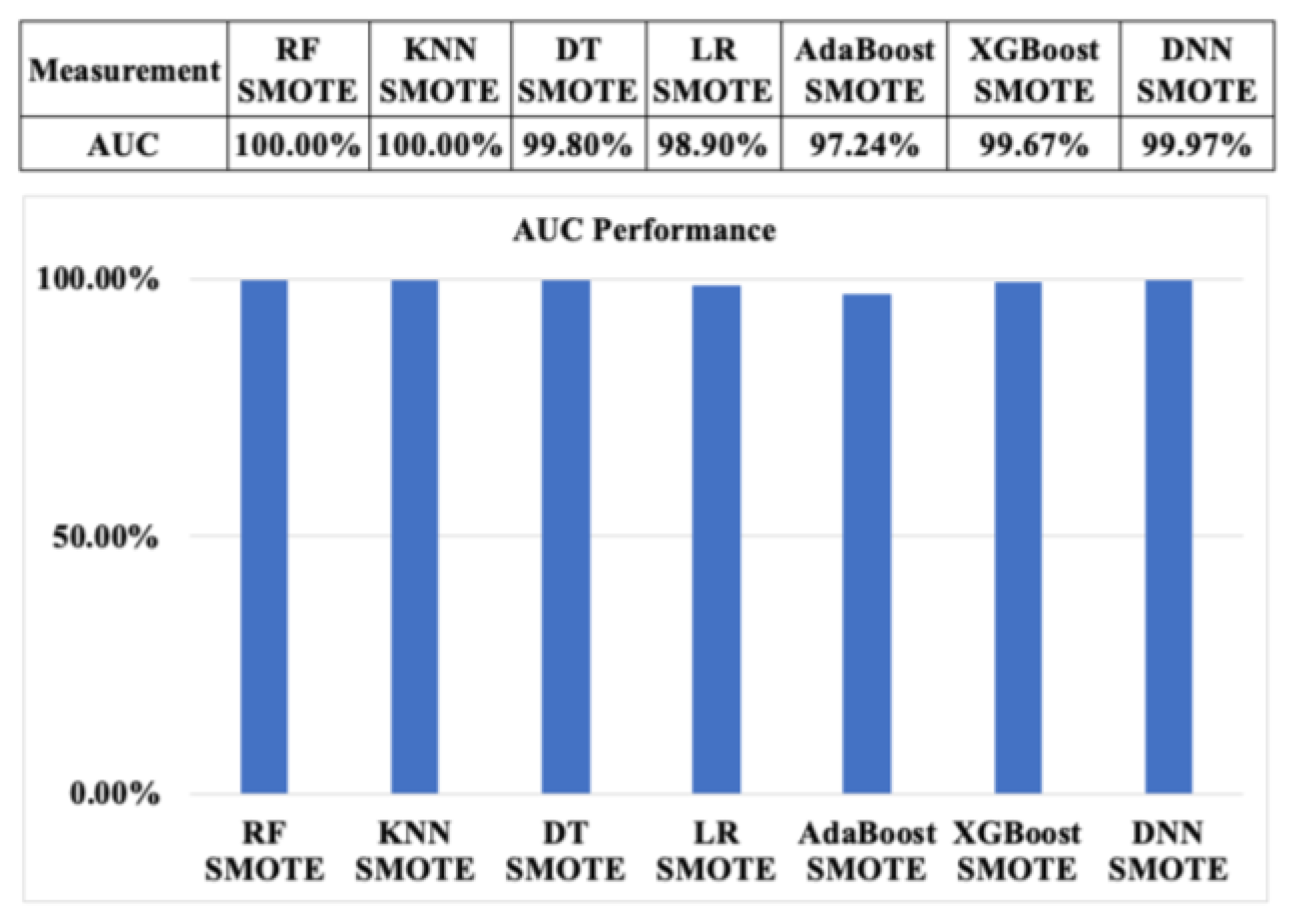
Finally, we also debate graphical assessment performance in order to make a sufficient evaluation of the CCF activities in this study. The comparisons of AUC of ML algorithms with SMOTE and ADSYN based on the resampling approach 1 are also described in Figure 16 and Figure 17, respectively. Based on Figure 16, the AUC of RF and KNN based on the SMOTE technique shows the highest results, at about 100%, whereas the AUC value of AdaBoost is relatively low, at about 97.24%.

Figure 16. AUC measurement performance of machine learning algorithms with SMOTE based on resampling approach 1.

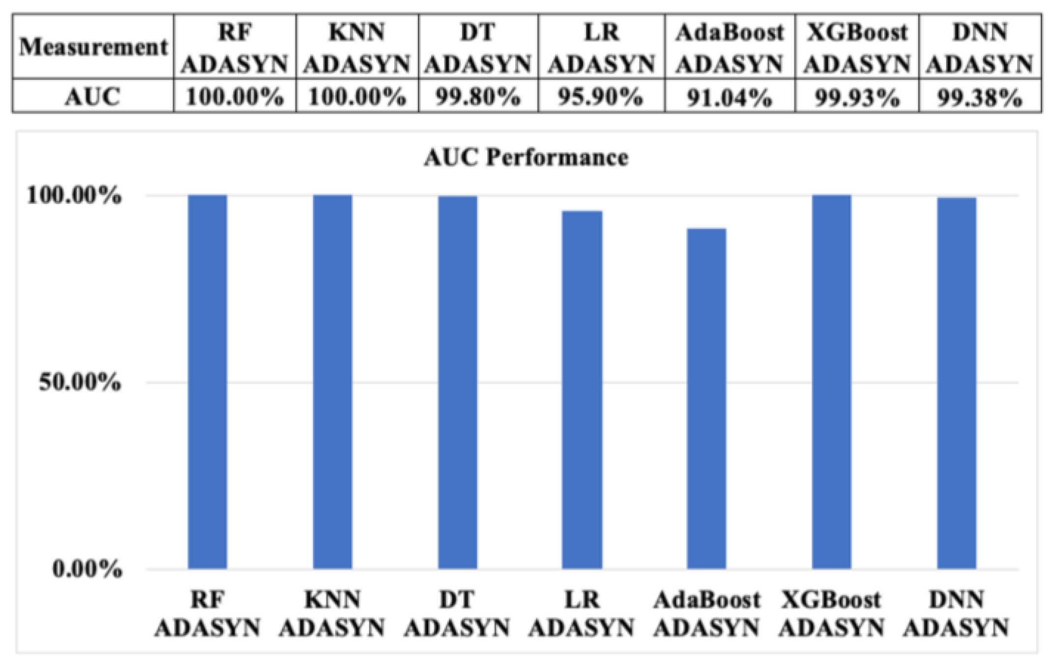
Figure 17. AUC measurement performance of machine learning algorithms with ADASYN based on resampling approach 1.

Additionally, as shown in Figure 17, the AUC results of seven ML algorithms with ADASYN also show the same trend as SMOTE, with approximately 100% of RF and KNN. This is followed by XGBoost, DT, and DNN, at approximately 99.93%, 99.8%, and 99.38%, respectively. AdaBoost also indicates the lowest value, at around 91.04%.

7.3. Results of Machine Learning Models Based on Resampling Approach 2

As indicated in Section 7.2, the results of the ML models of classification measurements indexes based on the resampling approach 1 are extremely good. In this section, we implement ML models based on the resampling approach 2 to analyze the reliability of the results mentioned in Section 7.2. The rates of the seven machine learning algorithms for CCF detection with SMOTE and ADASYN are illustrated in Table 10 and Table 11, respectively. Unlike the results of resampling approach 1, it is shown that the TP samples are less than the TN sample based on the ML algorithms.

Table 10. TP, FP, TN, FN rates of machine learning algorithms with SMOTE based on resampling approach 2.

Rate	RF with SMOTE	KNN with SMOTE	DT with SMOTE	LR with SMOTE	AdaBoost with SMOTE	XGBoost with SMOTE	DNN with SMOTE
TP	120	127	113	135	128	123	126
FP	14	127	168	2100	1086	37	180
TN	85,282	85,169	85,128	83,196	84,210	85,259	85,156
FN	27	20	34	12	19	24	21

Table 11. TP, FP, TN, FN rates of machine learning algorithms with ADASYN based on resampling approach 2.

Rate	RF with ADASYN	KNN with ADASYN	DT with ADASYN	LR with ADASYN	AdaBoost with ADASYN	XGBoost with ADASYN	DNN with ADASYN
TP	117	127	108	139	128	120	122
FP	13	128	150	7543	2670	44	134
TN	85,283	85,168	85,146	77,753	82,626	85,252	85,162
FN	30	20	39	8	19	27	25

The fundamental classification performance metrics of seven ML algorithms for CCF detection with SMOTE and ADASYN based on the resampling approach 2 are revealed in Figure 18 and Figure 19, respectively. According to Figure 18, the fundamental measurements indexes of RF with SMOTE are quite good at above 80%, whereas there is a significant difference between precision and other indexes in LR and AdaBoost with ADASYN. The precision of LR and AdaBoost is only about 6.04% and 10.54%. Similarly, as shown in Figure 19, RF with ADASYN also shows high outcomes in all indexes, while LR and AdaBoost with ADASYN show very low results of precision, at approximately 1.81% and 4.57%, respectively. These results are opposite to the ones based on the resampling approach 1. In general, the results of RF and XGBoost based on the resampling approach 2 are similar to their results with the resampling approach 1.

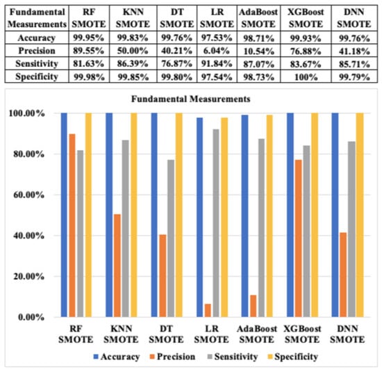
Figure 18. Fundamental classification performance measurements of ML algorithms with SMOTE based on resampling approach 2.

Figure 19. Fundamental classification performance measurements of ML algorithms with ADASYN based on resampling approach 2.

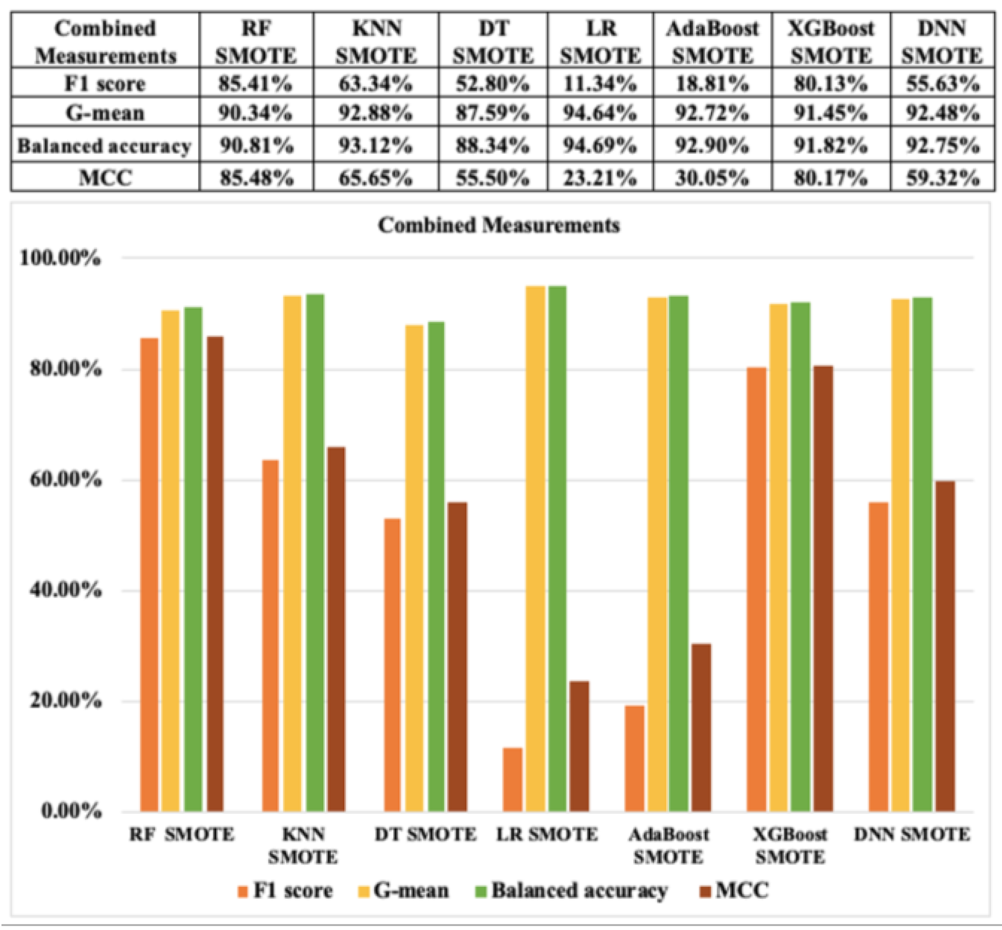
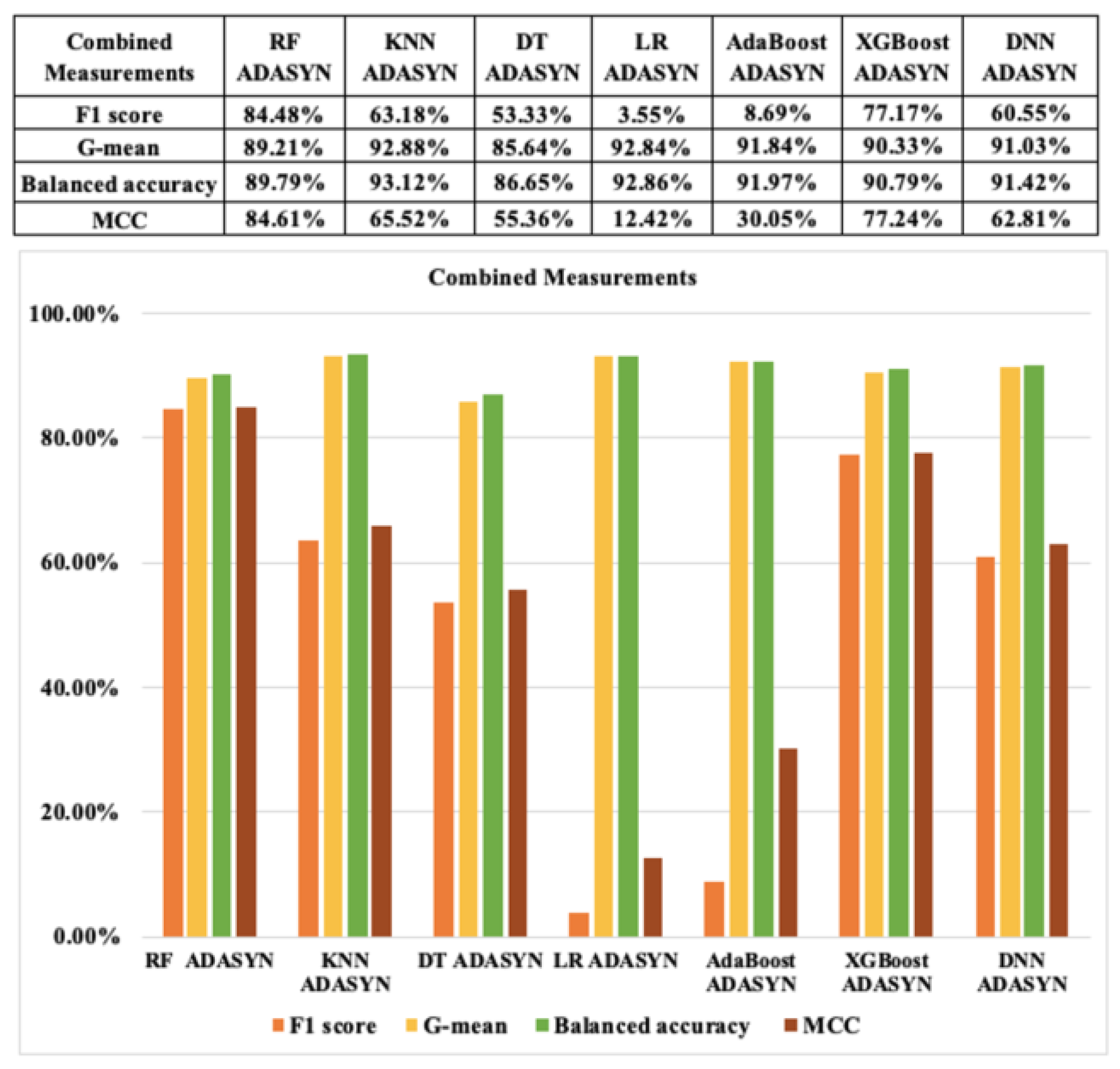
Moreover, as shown in Figure 20 and Figure 21, LR and AdaBoost with SMOTE and ADASYN based on the resampling approach 2 show a significant fluctuation among the indexes of combined metrics. The values of the G-mean and balanced accuracy are much higher than the F1 score and MCC values. The values of the F1 score are only about 11.34% and 18.81% based on LR and AdaBoost, respectively. Overall, RF and XGBoost show reliable results in terms of the combined metrics in both resampling approaches.

Figure 20. Combined classification performance measurements with SMOTE based on resampling approach 2.

Figure 21. Combined classification performance measurements with ADASYN based on resampling approach 2.

Based on the resampling approach 2, the positive likelihood ratios are indicated in Table 12. It is obvious that all model contributions are good, according to Table 3. However, there is a dramatic difference between these outcomes of models. The results of RF are very high, at approximately 4973.53, while LR shows very low results, at only 10.69. These results are similar to the ones based on the resampling approach 1.

Table 12. Positive Likelihood Ratio based on resampling approach 2.

ML Algorithms		Positive Likelihood Ratio	Model Contribution
RF	SMOTE	4973.53	Good
	ADASYN	5222.20	Good
KNN	SMOTE	580.24	Good
	ADASYN	575.71	Good
DT	SMOTE	390.28	Good
	ADASYN	417.78	Good
LR	SMOTE	37.30	Good
	ADASYN	10.69	Good
AdaBoost	SMOTE	68.39	Good
	ADASYN	27.82	Good
XGBoost	SMOTE	1928.92	Good
	ADASYN	1582.49	Good
DNN	SMOTE	406.36	Good
	ADASYN	528.28	Good

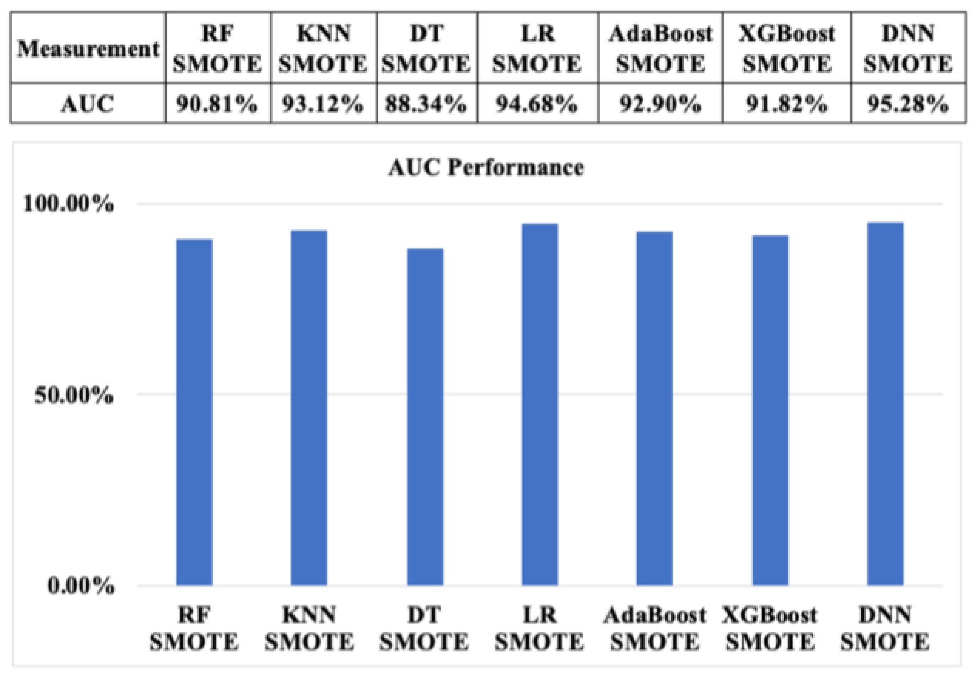
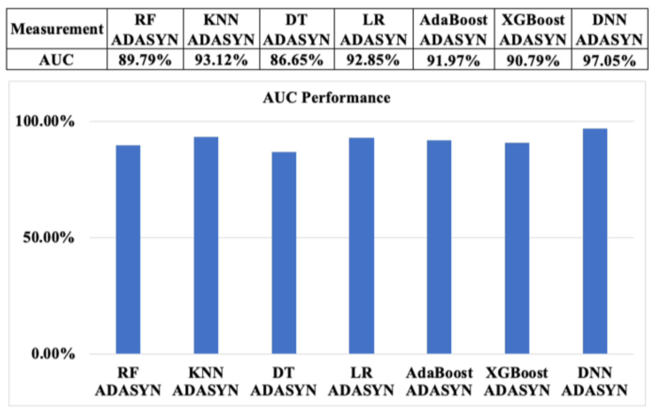
According to Figure 22 and Figure 23, AUC measurement performance of ML algorithms with SMOTE and ADASYN based on the resampling approach 2 show reliable outcomes, at above 86%. These outcomes are also quite similar to the AUC values based on approach 1.

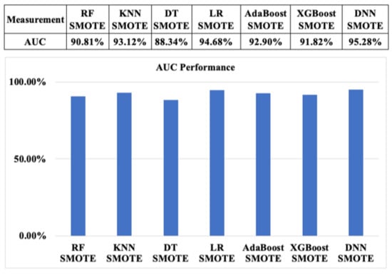
Figure 22. AUC measurement performance of machine learning algorithms with SMOTE based on resampling approach 2.

Figure 23. AUC measurement performance of machine learning algorithms with ADASYN based on resampling approach 2.

In general, the classification measurement indexes of ML algorithms for CCF detection based on SMOTE and ADASYN for the two resampling approaches are shown in Table 13 and Table 14, respectively. Based on these tables, we can see that the results of the resampling approach 2 are lower than the ones of the resampling approach 1, but still have a reliable degree. Moreover, RF and XGBoost show high performances with above 80% for all classification indexes. However, LR obtains a low performance, with 6.04% and 1.81% precision, and 11.34% and 3.55% F1 score for the resampling datasets based on SMOTE and ADASYN, respectively.

Table 13. Classification measurements indexes of ML algorithms based on SMOTE for two resampling approaches.

ML Algorithms Based on SMOTE	Accuracy	Precision	Sensitivity	Specificity	F1 Score	G-Mean	Balanced Accuracy	MCC	AUC
RF approach 1	99.99%	99.98%	100.00%	99.98%	99.99%	99.99%	99.99%	99.98%	100.00%
RF approach 2	99.95%	89.55%	81.63%	99.98%	85.41%	90.34%	90.81%	85.48%	90.81%
KNN approach 1	99.88%	99.76%	100.00%	99.75%	99.88%	99.88%	99.88%	99.76%	100.00%
KNN approach 2	99.83%	50.00%	86.39%	99.85%	63.34%	92.88%	93.12%	65.65%	93.12%
DT approach 1	99.78%	99.68%	99.87%	99.68%	99.78%	99.78%	99.78%	99.55%	99.80%
DT approach 2	99.76%	40.21%	76.87%	99.80%	52.80%	87.59%	88.34%	55.50%	88.34%
LR approach 1	94.51%	97.36%	91.51%	97.51%	94.34%	94.46%	94.51%	89.17%	98.90%
LR approach 2	97.53%	6.04%	91.84%	97.54%	11.34%	94.64%	94.69%	23.21%	94.68%
AdaBoost approach 1	97.24%	98.25%	96.20%	98.28%	97.21%	97.24%	97.24%	94.50%	97.24%
AdaBoost approach 2	98.71%	10.54%	87.07%	98.73%	18.81%	92.72%	92.90%	30.05%	92.90%
XGBoost approach 1	99.97%	99.94%	99.94%	100%	99.97%	99.97%	99.97%	99.94%	99.67%
XGBoost approach 2	99.93%	76.88%	83.67%	100%	80.13%	91.45%	91.82%	80.17%	91.82%
DNN approach 1	99.81%	99.69%	99.92%	99.69%	99.81%	99.81%	99.81%	99.61%	99.97%
DNN approach 2	99.76%	41.18%	85.71%	99.79%	55.63%	92.48%	92.75%	59.32%	95.28%

Table 14. Classification measurements indexes of ML algorithms based on ADASYN for two resampling approaches.

ML Algorithms Based on ADASYN	Accuracy	Precision	Sensitivity	Specificity	F1 Score	G-Mean	Balanced Accuracy	MCC	AUC
RF approach 1	99.98%	99.96%	100.00%	99.96%	99.98%	99.98%	99.98%	99.96%	100.00%
RF approach 2	99.95%	90.00%	79.59%	99.98%	84.48%	89.21%	89.79%	84.61%	89.79%
KNNapproach 1	99.90%	99.79%	100.00%	99.79%	99.90%	99.89%	99.89%	99.79%	100.00%
KNN approach 2	99.83%	49.80%	86.39%	99.85%	63.18%	92.88%	93.12%	65.52%	93.12%
DT approach 1	99.84%	99.75%	99.93%	99.74%	99.84%	99.84%	99.84%	99.67%	99.80%
DT approach 2	99.78%	41.86%	73.47%	99.82%	53.33%	85.64%	86.65%	55.36%	86.65%
LR approach 1	88.96%	91.12%	86.46%	91.48%	88.73%	88.94%	88.97%	77.23%	95.90%
LR approach 2	91.16%	1.81%	94.56%	91.16%	3.55%	92.84%	92.86%	12.42%	92.85%
AdaBoost approach 1	91.06%	97.97%	83.81%	98.27%	90.34%	90.75%	91.04%	82.98%	91.04%
AdaBoost approach 2	96.85%	4.57%	87.07%	96.87%	8.69%	91.84%	91.97%	30.05%	91.97%
XGBoost approach 1	99.93%	99.87%	100%	99.87%	99.93%	99.93%	99.93%	99.87%	99.93%
XGBoost approach 2	99.92%	73.17%	82%	99.95%	77.17%	90.33%	90.79%	77.24%	90.79%
DNN approach 1	99.69%	99.41%	99.96%	99.41%	99.69%	99.69%	99.69%	99.90%	99.38%
DNN approach 2	99.81%	47.66%	82.99%	99.84%	60.55%	91.03%	91.42%	62.81%	97.05%

7.4. Results of Deep Reinforcement for Imbalanced CCF Dataset

In this section, the performances of DRL for the imbalanced CCF dataset are discussed. The confusion matrix, which is shown in Table 15, illustrates that the TP samples are significantly less than the TN samples. The TP samples are just 37, while the TN samples are approximately 29,701.

Table 15. Confusion matrix of DRL on imbalanced dataset.

True Values	Predicted Values
	Class	0	1
	0	29,701	55,595
	110	34	37

Moreover, the classification metrics, such as accuracy, precision, sensitivity, F1 score, G-mean, and balance accuracy, for the DRL with the imbalanced CCF dataset are indicated in Table 16. It is obvious that the DRL does not have good performance in CCF detection. The accuracy index is only about 34.8%, and the precision index is very low, at just 0.067%. The value of the F1 score is also low, at about 13.27%. Generally, the results of the DRL for the imbalanced CCF classification do not indicate good performance compared with the performance of the ML classifiers based on the balanced CCF dataset.

Table 16. Classification metrics for DRL on imbalanced CCF dataset.

Classification Measurements	Accuracy	Precision	Sensitivity	Specificity	F1 Score	G-Mean	Balanced Accuracy
	34.8%	0.067%	25.17%	34.82%	13.27%	29.60%	29.99%

8. Conclusions and Future Works

In this study, we comprehensively analyze the imbalanced CCF dataset through the DRL and the ML algorithms. It is due to the fact that these analyses are considered as one of the crucial factors in building the speed and effectiveness of the system detection of CCF. First, the processing data stage is applied to this CCF dataset to increase the effectiveness of these models. Second, we resample the imbalanced CCF dataset based on two simple but effective resampling techniques, i.e., SMOTE and ADSYN through two resampling approaches: resampling approach 1 and resampling approach 2. The difference between the resampling approach 1 and the resampling approach 2 is the position where SMOTE and ADASYN are used to resample the imbalanced CCF datasets. These ML algorithms are then applied to the balanced CCF datasets, which are accomplished from SMOTE and ADASYN based on the two resampling approaches. Next, the distinguishing classification evaluation indexes are utilized to prove the effectiveness of the models of CCF detection. The classification metrics consist of three primary types, known as fundamental, combined, and graphical assessments. Through our experiments, all of the results of the indexes of the classification metrics are nearly perfect in the resampling approach 1. However, in the resampling approach 2, the results have a big gap among the indexes. This is mainly because that resampling is performed for the full sample in the resampling approach 1. Based on the resampling approach 2, the precision, F1 score, and MCC show low results in LR and AdaBoost, while RF and XGBoost represent stable results in all the indexes of classification metrics. Furthermore, it is obvious that the results of the ML classifiers for CCF detection that are based on the SMOTE technique are better than the results which are based on the ADASYN algorithm. This is mainly because ADASYN has two weaknesses. The first weakness is each neighborhood can only include one minority example in terms of minority examples sparsely distributed. The second one is that the accuracy of this technique suffers owing to its adaptable nature [44]. Finally, the DRL, which is considered as the novel approach, is used for the imbalanced CCF dataset, but it does not accomplish results that are as good as we expected.

In conclusion, our comprehensive empirical results with the imbalanced CCF datasets in the banking sector have shown that the performance metrics of ML algorithms based on two resampling approaches are better than that of DRL with the imbalanced dataset. RF and XGBoost are considered as the best approaches to cope with the CCF dataset based on two resampling approaches. On the other hand, TP and TN rates based on two resampling approaches show an opposite trend. The rates of TP are greater than the TN rates based on the resampling approach 1, while the rates of TP are less than the TN rates in the resampling approach 2. This leads to unexpected results for detecting CCF in several indexes of classification measurements in the resampling approach 2.

In the future, we want to collect precisely and extend the dataset through financial companies to accomplish an exhaustive model. We continue to improve the credit card fraud detection system through other different ML and deep learning approaches. In addition, extending and applying ML techniques over highly imbalanced datasets to other application domains, like big data sampling and clustering [45], recommendation systems [46], and security and privacy issues [47] with deep learning, is also of great interest to us in the future. Additionally, we consider using the Leave-One-Out Cross-Validation approach rather than the train/test split using a ratio of 7:3 to enhance the robust performance of detecting CCF using ML algorithms [48]. We also employ the Brier Score, which is a useful metric of classifier performance to evaluate the ML models in terms of losses in future research [20]. Furthermore, we will implement real applications for the banking sector.

References

- Nilsonreport. Available online: https://nilsonreport.com/publication_newsletter_archive_issue.php?issue=1187 (accessed on 22 May 2021).
- Sisodia, D.S.; Reddy, N.K.; Bhandari, S. Performance Evaluation of Class Balancing Techniques for Credit Card Fraud Detection. In Proceedings of the 2017 IEEE International Conference on Power, Control, Signals and Instrumentation Engineering (ICPCSI), Chennai, India, 21–22 September 2017. [Google Scholar]
- Zhu, B.; Baesens, B.; vanden Broucke, S.K. An empirical comparison of techniques for the class imbalance problem in churn prediction. Inf. Sci. 2017, 408, 84–99. [Google Scholar] [CrossRef] [Green Version]
- Lin, E.; Chen, Q.; Qi, X. Deep reinforcement learning for imbalanced classification. Appl. Intell. 2020, 50, 2488–2502. [Google Scholar] [CrossRef] [Green Version]
- Tran, T.C.; Dang, T.K. Machine Learning for Prediction of Imbalanced Data: Credit Fraud Detection. In Proceedings of the 2021 15th International Conference on Ubiquitous Information Management and Communication (IMCOM), Seoul, Korea, 4–6 January 2021; pp. 1–7. [Google Scholar]
- Padmaja, T.M.; Dhulipalla, N.; Bapi, R.S.; Krishna, P. Unbalanced Data Classification Using extreme outlier Elimination and Sampling Techniques for Fraud Detection. In Proceedings of the 15th International Conference on Advanced Computing and Communications (ADCOM), Guwahati, India, 18–21 December 2007; pp. 511–516. [Google Scholar]
- Kumari, P.; Mishra, S.P. Analysis of Credit Card Fraud Detection Using Fusion Classifiers. Adv. Intell. Syst. Comput. 2018, 711, 111–122. [Google Scholar]
- Brause, R.; Langsdorf, T.; Hepp, M. Neural Data Mining for Credit Card Fraud Detection. In Proceedings of the Proceedings 11th International Conference on Tools with Artificial Intelligence, Chicago, IL, USA, 9–11 November 1999. [Google Scholar]
- Srivastava, A.; Kundu, A.; Sural, S.; Majumdar, A.K. Credit Card Fraud Detection Using Hidden Markov Model. IEEE Trans. Depenable Secur. Comput. 2008, 5, 37–48. [Google Scholar] [CrossRef]
- Raj, S.B.E.; Portia, A.A. Analysis on Credit Card Fraud Detection Methods. In Proceedings of the 2011 International Conference on Computer, Communication and Electrical Technology (ICCCET), Tamilnadu, India, 18–19 March 2011. [Google Scholar]
- Li, Z.; Huang, M.; Liu, G.; Jiang, C. A hybrid method with dynamic weighted entropy for handling the problem of class imbalance with overlap in credit card fraud detection. Expert Syst. Appl. 2021, 175, 114750. [Google Scholar] [CrossRef]
- Fatima, E.B.; Omar, B.; Abdelmajid, E.M.; Rustam, F.; Mehmood, A.; Choi, G.S. Minimizing the overlapping degree to improve class-imbalanced learning under sparse feature selection: Application to fraud detection. IEEE Access 2021, 9, 28101–28110. [Google Scholar] [CrossRef]
- Makki, S.; Assaghir, Z.; Taher, Y.; Haque, R.; Hacid, M.; Zeineddine, H. An Experimental Study With Imbalanced Classification Approaches for Credit Card Fraud Detection. IEEE Access 2019, 7, 93010–93022. [Google Scholar] [CrossRef]
- Mittal, S.; Tyagi, S. Performance Evaluation of Machine Learning Algorithms for Credit Card Fraud Detection. In Proceedings of the 2019 9th International Conference on Cloud Computing, Data Science & Engineering (Confluence), Noida, India, 10–11 January 2019. [Google Scholar]
- Uddin, M.F. Addressing Accuracy Paradox Using Enhanched Weighted Performance Metric in Machine Learning. In Proceedings of the 2019 Sixth HCT Information Technology Trends (ITT), Ras Al Khaimah, United Arab Emirates, 20–21 November 2019. [Google Scholar]
- Valverde-Albacete, F.J.; Peláez-Moreno, C. 100% Classification Accuracy Considered Harmful: The Normalized Information Transfer Factor Explains the Accuracy Paradox. PLoS ONE 2014, 9, e84217. [Google Scholar] [CrossRef] [Green Version]
- Kaggle. Credit Card Fraud Detection Anonymized Credit Card Transactions Labeled as Fraudulent or Genuine. Available online: https://www.kaggle.com/mlg-ulb/creditcardfraud (accessed on 2 September 2020).
- Zhu, R.; Guo, Y.; Xue, J.H. Adjusting the Imbalance Ratio by the Dimensionality of Imbalanced Data. Pattern Recognit. Lett. 2020, 133, 217–223. [Google Scholar] [CrossRef]
- Towards Data Science. Available online: https://towardsdatascience.com/scale-standardize-or-normalize-with-scikit-learn-6ccc7d176a02 (accessed on 5 September 2020).
- Fernández, A.; García, S.; Galar, M.; Prati, R.C.; Krawczyk, B.; Herrera, F. Learning from Imbalanced Data Sets; Springer: Cham, Switzerland, 2018. [Google Scholar]
- Li, K.; Zhang, W.; Lu, Q.; Fang, X. An Improved SMOTE Imbalanced Data Classification Method Based on Support Degree. In Proceedings of the 2014 International Conference on Identification, Information and Knowledge in the Internet of Things, Beijing, China, 17–18 October 2014; pp. 34–38. [Google Scholar]
- Demidova, L.; Klyueva, I. SVM Classification: Optimization with the SMOTE Algorithm for the Class Imbalance Problem. In Proceedings of the 2017 6th Mediterranean Conference on Embedded Computing (MECO), Bar, Montenegro, 11–15 June 2017. [Google Scholar]
- Lu, C.; Lin, X.L.S.; Shi, H. Telecom Fraud Identification Based on ADASYN and Random Forest. In Proceedings of the 2020 5th International Conference on Computer and Communication Systems (ICCCS), Shanghai, China, 15–18 May 2020. [Google Scholar]
- Chawla, N.V.; Bowyer, K.W.; Hall, L.O.; Kegelmeyer, W.P. SMOTE: Synthetic Minority Over-Sampling Technique. Artif. Intell. Res. 2002, 16, 321–357. [Google Scholar] [CrossRef]
- Last, F.; Douzas, G.; Bacao, F. Oversampling for Imbalanced Learning Based on K-Means and SMOTE. arXiv 2017, arXiv:1711.00837. [Google Scholar]
- He, H.; Bai, Y.; Garcia, E.A.; Li, S. ADASYN: Adaptive Synthetic Sampling Approach for Imbalanced Learning. In Proceedings of the 2008 IEEE International Joint Conference on Neural Networks (IEEE World Congress on Computational Intelligence), Hong Kong, China, 1–8 June 2008; pp. 1322–1328. [Google Scholar]
- Leo, M.; Sharma, S.; Maddulety, K. Machine Learning in Banking Risk Management: A Literature Review. Risks 2019, 7, 29. [Google Scholar] [CrossRef] [Green Version]
- Belmonte, J.L.; Segura-Robles, A.; Moreno-Guerrero, A.-J.; Parra-González, M.E. Machine Learning and Big Data in the Impact Literature. A Bibliometric Review with Scientific Mapping in Web of Science. Symmetry 2020, 12, 495. [Google Scholar] [CrossRef] [Green Version]
- Beckonert, O.; Bollard, M.E.; Ebbels, T.M.; Keun, H.C.; Antti, H.; Holmes, E.; Lindon, J.C.; Nicholson, J.K. NMR-based Metabonomic Toxicity Classification: Hierarchical Cluster Analysis and K-Nearest-Neighbour Approaches. Anal. Chim. Acta 2003, 490, 3–15. [Google Scholar] [CrossRef]
- Alsbergav, B.; Goodacrea, R.; Rowlandb, J.; Kella, D. Classification of Pyrolysis Mass Spectra by Fuzzy Multivariate Rule Induction-Comparison with Regression, K-Nearest Neighbour, Neural and Decision-Tree Methods. Anal. Chim. Acta 1997, 348, 389–407. [Google Scholar] [CrossRef]
- Urso, A.; Fiannaca, A.; La Rosa, M.; Ravì, V.; Rizzo, R. Data Mining: Prediction Methods. Encycl. Bioinform. Comput. Biol. 2019, 1, 413–430. [Google Scholar]
- Quinlan, J.R. Induction of Decision Trees. Mach. Learn. 1986, 1, 81–106. [Google Scholar] [CrossRef] [Green Version]
- Quinlan, J.R. C4.5: Programs for Machine Learning; Morgan Kaufmann Publishers: San Mateo, CA, USA, 1993. [Google Scholar]
- Builtin.com. A Complete Guide to the Random Forest Algorithm. Available online: https://builtin.com/data-science/random-forest-algorithm (accessed on 22 May 2021).
- Ho, T.K. Random Decision Forests. In Proceedings of the ICDAR ’95: Proceedings of the Third International Conference on Document Analysis and Recognition, Montreal, QC, Canada, 14–16 August 1995. [Google Scholar]
- Breiman, L. Random Forests. Mach. Learn. 2001, 45, 5–32. [Google Scholar] [CrossRef] [Green Version]
- Hassan, A.R.; Haque, M.A. Computer-Aided Obstructive Sleep Apnea Screening from Single-Lead Electrocardiogram using Statistical and Spectral Features and Bootstrap Aggregating. Biocybern. Biomed. Eng. 2016, 36, 256–266. [Google Scholar] [CrossRef]
- Zhao, D. Comparative Analysis of Different Characteristics of Automatic Sleep Stages. Comput. Methods Programs Biomed. 2019, 175, 53–72. [Google Scholar] [CrossRef]
- Chen, T.; Guestrin, C. XGBoost: A scalable Tree Boosting System. In Proceedings of the 22nd ACM SIGKDD International Conference on Knowledge Discovery and Data Mining—KDD ’16; ACM Press: San Francisco, CA, USA, 2016. [Google Scholar]
- Towardsdatascience. Available online: https://towardsdatascience.com/https-medium-com-vishalmorde-xgboost-algorithm-long-she-may-reinedd9f99be63d#:~:text=XGBoost%20is%20a%20decision%2Dtree,all%20other%20algorithms%20or%20frameworks (accessed on 22 May 2021).
- Yuvaraj, N.; Raja, R.A.; Kousik, N.V.; Johri, P.; Diván, M.J. Analysis on the Prediction of Central Line-Associated Bloodstream Infections (CLABSI) using Deep Neural Network Classification. Comput. Intell. Appl. Healthc. 2020, 229–244. [Google Scholar]
- Sokolova, M.; Lapalme, G. A Systematic Analysis of Performance Measures for Classification Tasks. Inf. Process. Manag. 2009, 45, 427–437. [Google Scholar] [CrossRef]
- Bekkar, M.; Djemaa, H.K.; Alitouche, T.A. Evaluation Measures for Models Assessment over Imbalanced Data Sets. J. Inf. Eng. Appl. 2013, 3, 27–38. [Google Scholar]
- Medium.com. Fixing Imbalanced Datasets: An Introduction to ADASYN (with code!). Available online: https://medium.com/@ruinian/an-introduction-to-adasyn-with-code-1383a5ece7aa (accessed on 22 May 2021).
- Hoang, N.L.; Trang, L.H.; Dang, T.K. A Comparative Study of the Some Methods Used in Constructing Coresets for Clustering Large Datasets. SN Comput. Sci. 2020, 1, 1–12. [Google Scholar] [CrossRef]
- Dang, T.K.; Nguyen, Q.P.; Nguyen, V.S. Evaluating Session-Based Recommendation Approaches on Datasets from Different Domains. In International Conference on Future Data and Security Engineering; Springer: Cham, Switzerland, 2019; pp. 577–592. [Google Scholar]
- Ha, T.; Dang, T.K.; Dang, T.T.; Truong, T.A.; Nguyen, M.T. Differential Privacy in Deep Learning: An Overview. In Proceedings of the 2019 International Conference on Advanced Computing and Applications (ACOMP), Nha Trang, Vietnam, 26–28 November 2019. [Google Scholar]
- Sharan, R.V.; Berkovsky, S.; Taib, R.; Koprinska, I.; Detecting, J.L. Personality Traits Using Inter-Hemispheric Asynchrony of the Brainwaves. In Proceedings of the 2020 42nd Annual International Conference of the IEEE Engineering in Medicine & Biology Society (EMBC), Montreal, QC, Canada, 20–24 July 2020. [Google Scholar]
Publisher’s Note: MDPI stays neutral with regard to jurisdictional claims in published maps and institutional affiliations. |
© 2021 by the authors. Licensee MDPI, Basel, Switzerland. This article is an open access article distributed under the terms and conditions of the Creative Commons Attribution (CC BY) license (https://creativecommons.org/licenses/by/4.0/).