Abstract
Geosynthetic-reinforced soil (GRS) technology has been used worldwide since the 1970s. An extension to its development is the application as a bridge abutment, which was initially developed by the Federal Highway Administration (FHWA) in the United States, called the GRS—integrated bridge system (GRS-IBS). Now, there are several variations of this technology, which includes the GRS Integral Bridge (GRS-IB) developed in Japan in the 2000s. In this study, the GRS-IB and GRS-IBS are examined. The former uses a GRS bridge abutment with a staged-construction full height rigid (FHR) facing integrated to a continuous girder on top of the FHR facings. The latter uses a block-faced GRS bridge abutment that supports the girders without bearings. In addition, a conventional integral bridge (IB) is considered for comparison. The numerical analyses of the three bridges using Plaxis 2D under static and dynamic loadings are presented. The results showed that the GRS-IB exhibited the least lateral displacement (almost zero) at wall facing and vertical displacements increments at the top of the abutment compared to those of the GRS-IBS and IB. The presence of the reinforcements (GRS-IB) reduced the vertical displacement increments by 4.7 and 1.3 times (max) compared to IB after the applied general traffic and railway loads, respectively. In addition, the numerical results revealed that the GRS-IB showed the least displacement curves in response to the dynamic load. Generally, the results revealed that the GRS-IB performed ahead of both the GRS-IBS and IB considering the internal and external behavior under static and dynamic loading.
1. Introduction
The concept of reinforced soil is not new and is believed to have already existed since the 5th and 4th millenniums BC. Primeval people used reeds, straw, branches, or sticks as reinforcements [,,]. Around the early 1970s, geotextiles were used as reinforcements. One of the first geotextile-reinforced walls in the United States was built in Siskiyou National Forest, Oregon. In 1971, the first geotextile-reinforced soil was constructed in France for improving embankment stability. A similar structure was first constructed in the United States in 1974. Around the early 1980s, geogrids were developed and used as soil reinforcements. In 1981, the first geogrid-reinforced earth was used. The extensive use in the United States began in about 1983 [,,,,,]. The technology has been widely used as temporary support on permanent roadway embankments. Since then, there has been a significant increase on the application of geosynthetic-reinforced soil.
In the United States, the application of geosynthetic-reinforced soil (GRS), a retaining wall (RW) as a bridge abutment was initially developed by the Federal Highway Administration (FHWA), called the GRS—integrated bridge system (GRS-IBS). There are several variations of this technology. Typically, the GRS-IBS includes a GRS abutment, reinforced soil foundation (RSF), bearing bed reinforcement, bridge seat, and an integrated approach (see Figure 1). The RSF is composed of granular fill material that is compacted and encapsulated with a geotextile. It increases the bearing capacity and width of the GRS abutment. The GRS abutment uses alternating backfill layers that are well-compacted and short-spaced geosynthetic reinforcement to provide support for the bridge. The bridge is placed directly on the bridge seat of the GRS abutment without joints or the use of bearing. Under the bridge seat is the bearing bed reinforcement zone, which provides support for the bridge loads. This technology also has an integrated approach that provides a smooth transition without joints between the superstructure and alleviates the problem on the differential settlement between bridge abutments and approach roadways [,].
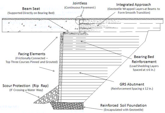
Figure 1.
Typical GRS—integrated bridge system [].
In Japan, a GRS RW with staged-construction FHR facing was developed in the mid-1980s. Since 1987, a large number of permanent GRS retaining walls (RWs) with FHR facings have been built supporting railways, including the high-speed train lines in Japan. An extension of this technology was then developed in the 2000s as a bridge abutment. There are a couple of new bridge systems that have been replacing the conventional-type bridges which use the GRS technology developed. One example concerns the GRS integral bridge (GRS-IB) technology, which includes a continuous girder wherein both ends are structurally connected without using bearings to the top of the FHR facing of a pair of GRS RWs. The GRS-IB technology alleviates the technical problems of conventional bridges, solving the problems of RC structures by eliminating the bearings and joints, and has solved several problems related to the backfill through the use of geosynthetic reinforcement. The GRS-IB composed of a GRS RW as a bridge abutment with a staged-construction full height rigid (FHR) facing and integrated with the continuous reinforced concrete (RC) girder on top of the FHR facing without bearings and joint is depicted in Figure 2 [,,,,,].
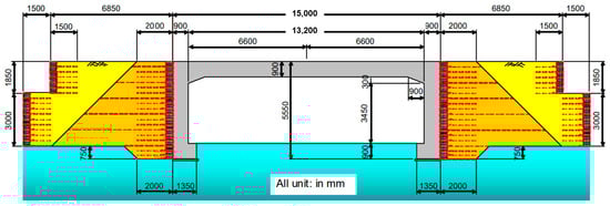
Figure 2.
GRS integral bridge full-scale model design [].
The GRS-IBS and GRS with FHR have been adopted by advanced countries in Asia as well as in Europe, overthrowing the conventional bridges because of its economical, construction, and structural advantages [,,,,,]. In the Philippines, no literature has shown that this technology has been used to date. Thus, the authors envisioned the use an integral bridge (IB) using geosynthetic-reinforced soil (GRS) with full height rigid (FHR) facing bridge abutment in the Philippines, which is prone to severe earthquakes. Thus, a comparative study on the behavior of GRS-IB is undertaken to have first-hand proof of its advantages over the other type of bridges using numerical analysis.
2. Numerical Modelling Using Plaxis 2D
2.1. Description of the Bridge Models
In this study, there are three types of bridges that are presented (see Figure 3): (1) Case 1, GRS-IB, an integral bridge with a GRS RW bridge abutment and FHR facing; (2) Case 2, GRS-IBS, an integrated bridge system with a GRS RW bridge abutment supporting the simply supported bridge girders with no bearings; and (3) Case 3, a typical integral bridge (IB) with an unreinforced bridge abutment. The three different bridge technologies are designed and analyzed using the finite element method (FEM) in the Plaxis 2D (AE.02 Version 2013) program under static and dynamic loads. A detailed description for each model case is provided in the following subsections.
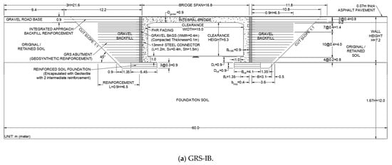
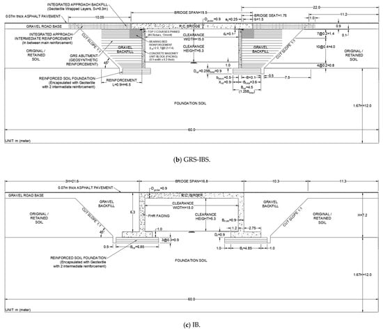
Figure 3.
Design details of each model case: (a) GRS-IB; (b) GRS-IBS; and (c) IB Model.
2.1.1. GRS-IBS Model Design
The GRS-IBS model is designed according to FHWA-HRT-11-026 [] and is checked to satisfy the internal and external stability based on Das [], FHWA-HRT-11-026 [], FHWA-HRT-11-027 [], FHWA-NHI-10-024 [], and Murthy [] (see Figure 3b). The GRS-IBS includes a GRS abutment, reinforced soil foundation (RSF), bearing bed reinforcement, bridge seat, and an integrated approach. In this study, the bridge is assumed to have a clear span length of 15.0 m in order to accommodate four-lane traffic under the bridge and a clear height of 5.3 m, just enough to pass the FHWA minimum vertical clearance for roadways which is specified as 4.3–4.9 m. The bearing width (b) used is 1.5 m (>0.762 m minimum), similar to the design of Maree Michel’s GRS IBS []. The setback distance () between the back of the wall facing and the beam seat used is 250 mm. The minimum clear space (de) or gap between the top of the uppermost facing block and the bottom of the girder (superstructure) is considered to be 100 mm (>76 mm min). The minimum base width including the block face (Btotal) for the bridge span length (Lspan) greater than 7.62 m (25 ft) is 1.83 m (6 ft). The author chose Btotal = 3.6 m (≈0.6 H), which also satisfies the minimum base-to-height (Btotal/H) ratio of 0.3. The RSF is composed of granular fill material that is compacted and encapsulated with geotextile. The depth of the excavation for the RSF (DRSF) is equal to 0.25 Btotal = 0.9 m. The total width of the RSF (BRSF) is equal to 4.5 m, which extends in front of the wall face by one-fourth of the width of the base. In this study, there are two intermediate reinforcements added inside the RSF, similar to the design of Maree Michel’s GRS-IBS []. The length of the lowest reinforcement layer at the base of the abutment is equal to 3.6 m (0.43 H), which is more than the width of the base (B = 3.1 m, excluding the block face) but more than the minimum base-to-height (B/H) ratio (excluding the block face) of 0.3. The CMU blocks used in this study have a width of 0.5 m and thickness of 0.2 m. Ardah et al. [] specifies that after the base length of the reinforcement has been chosen (in this case it is equal to 3.6 m), the reinforcement length should follow the cut slope (in this study it is assumed to be 1:1) up to a B/H ratio of 0.7. In this study, the length of the uppermost reinforcement layer in the abutment is assumed to be equal to 6.5 m (0.9 H), which is higher than the recommended. From the base, the reinforcement length can become progressively longer in the reinforcement zones. The vertical spacing between reinforcements is assumed to be 0.2 m for the first four layers from the base and then 0.4 m for the succeeding layers until the bottom layer of the bearing reinforcement zone. Then, the vertical spacing for the main reinforcement layers at the final zone is 0.2 m. A bearing reinforcement zone is added underneath the bridge seat to support the bridge loads. The vertical spacing for the bearing bed reinforcement is half the primary vertical spacing, which is 0.1 m. The bearing bed reinforcement length is equal to 2.0 m, which is two times the setback () plus the width of the bridge seat (b). In this study, there are six bearing bed reinforcement layers, which is sufficient and more than the stipulated minimum. At the integrated approach, the gravelly backfill layers at the beams are wrapped with geotextiles without joints to form a smooth transition from the bridge superstructure. One intermediate reinforcement is added between the main integrated approach reinforcement layers. Here, there are three wrapped layers with a height of 0.30 m and the total reinforcement length is 10 m from the face of the superstructure (girder). The reinforcement length extends 1 m beyond the cut and slope to reduce the differential settlement between the backfill soil and the cut slope. The final design and detailed specification of the GRS-IBS model is depicted in Figure 3b.
2.1.2. GRS-IB Model Design
In this study, the GRS-IB model is a modified design based on the full-scale model in Japan [,] and the created model of GRS-IBS in this study. The IB design of the former and the GRS RW abutment configuration of the latter are combined to complete the GRS-IB model design for this study. The final design and detailed specifications of the GRS-IB model is depicted in Figure 3a. The GRS-IB also has a clear span length of 15.0 m and a clear height of 5.3 m, similar to the GRS-IBS. The GRS-IB includes a GRS abutment, RSF, FHR facing, and RC footing. The FHR facing is the substructure that is continuously connected to the superstructure, which is the RC bridge girder, eliminating the joints and bearing, thus forming an integral bridge structure. The FHR facing has a width of 0.9 m and its footing has width of 1.35 m and thickness of 0.9 m. The RSF underneath the base of the GRS-IB has dimensions and reinforcements similar to those of the GRS-IBS. The RSF extends by 1.0 m from the toe of the FHR footing. Moreover, in order to have a similar condition with the GRS-IBS model, the abutment has a cut slope of 1:1 and the same reinforcement quantity, spacing, and lengths are used for the GRS-IB model, except for the intermediate reinforcements at the bearing bed zone. The GRS-IB model does not include a bridge seat, thus the bearing reinforcement zone is not needed. The bridge loads are supported directly by the FHR facing. The FHR facing is connected to the GRS RW abutment. The abutment uses gravel bags that are placed at the facing, compacted to a thickness of 0.1 m and width of 0.4 m. The lowest and uppermost reinforcement layer zones include two wrapped layers of gravel bags, while the middle reinforcement layer zone includes four wrapped layers of gravel bags. The steel reinforcements are added to connect the GRS RW and FHR facing. The steel reinforcement has a vertical spacing of 0.4 m and horizontal spacing of 0.15 m.
2.1.3. IB Model Design
The IB model is included in this study in order to show the effects of having an IB system but without the reinforcements in the abutment. The configuration of the IB model is based from the GRS-IB model, which includes a RSF, FHR facing, and RC footing. The final design and detailed specification of the IB model is depicted in Figure 3c. The IB also has a clear span length of 15.0 m and a clear height of 5.3 m, similar to the GRS-IBS and GRS-IB models. Here, the FHR facing has a width of 0.9 m and its footing has a width of 4.85 m and thickness of 0.9 m. In this case, the RSF extends by 1.0 m from the toe of the FHR footing and 1.0 m from the heel of the FHR footing. The FHR footing is wider than the GRS-IB model because it has no GRS abutment.
2.2. Geometry Configuration of Each Model Case
Modelling the entire bridge design for the numerical analysis may be too complex and time consuming. Therefore in this study, only the right-hand side of the bridge and abutment are considered. This method of modelling the free-standing geometry of the bridge abutment was also done by Abu-Farsakh et al. [,], Ardah et al. [,], and Zheng and Fox []. As a result, the right-hand side model of each bridge is depicted in Figure 4, Figure 5 and Figure 6. To validate the method of modelling the free-standing geometry of the bridge abutment using the Plaxis 2D version, numerical analyses were conducted with reference data from Ardah et al. [] and the results showed a good agreement with very minimal difference.
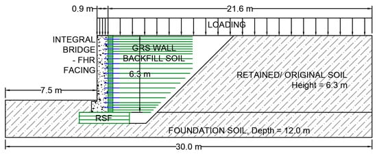
Figure 4.
Plaxis 2D numerical model configuration for GRS-IB (Case 1).
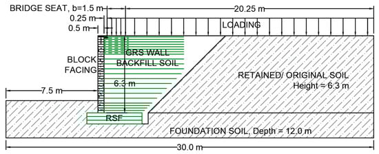
Figure 5.
Plaxis 2D numerical model configuration for GRS-IBS (Case 2).
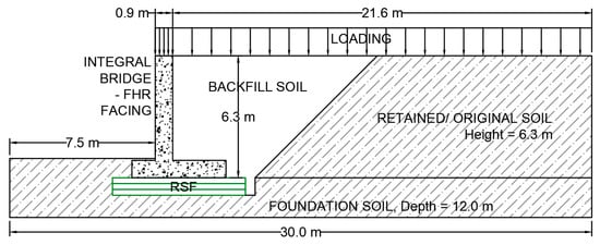
Figure 6.
Plaxis 2D numerical model configuration for IB (Case 3).
Considering the right-hand side of the bridge and abutment, the 0.90-m thick integrated approach backfill and the 0.90-m thick RC bridge girder are removed and converted into its equivalent vertical loads. Thus, the height of the abutment is left at 6.3 m from the base. The models are designed with enough horizontal and vertical distance from the right-end and bottom boundaries, respectively. The horizontal distance from the right-end to the wall facing is more than three times the height of the wall. The vertical distance from the base of wall to the bottom boundary is almost twice the height of the wall. The front-end is 7.5 m from the wall facing because this is the half-point of the bridge (with a clear width of 15 m). Consequently, the boundary conditions are modelled wherein the vertical sides of the models at X = 0 and X = 30 are fixed on the X-direction, while the bottom boundary at Y = −12 is fixed on both the X and Y-directions. In other words, a fixed boundary condition is applied at the bottom of the model while a roller boundary condition is applied on both sides of the model. The FE models of the bridges are simulated in Plaxis 2D based on the example procedures in the Plaxis 2D Reference and Tutorial Manuals [,] as well as on a few related literature studies including Abu-Farsakh et al. [,], Ardah et al. [,], Koda et al. [], Tatsuoka et al. [], and Yazaki et al. [].
For the mesh condition, all models used a plane strain model with 15-noded triangular elements, which are the default setting in Plaxis 2D. After the mesh generation, the Case 1 numerical model (GRS-IB) had a total of 49,687 nodes and 5441 soil elements with an average element size of 0.3176 m. The Case 2 numerical model (GRS-IBS) had a total of 56,730 nodes and 6284 soil elements with an average element size of 0.2956 m. Lastly, the Case 3 numerical model (IB) had a total of 32,762 nodes and 3915 soil elements with an average element size of 0.3745 m. The number of nodes and elements differ from each numerical model because the mesh depends on the geometry of the numerical model.
2.3. Material Input Parameters
2.3.1. Soil Material Input Parameters
There are three main soil materials that are used in this study. One is the backfill soil, which is assumed to be a granular or gravelly material. The constitutive model used to simulate the behavior of the soil backfill is the hardening soil (HS). The HS model is an advanced model for the simulation of soil behavior []. The HS model is an elastoplastic type of hyperbolic model that accounts for the stress-dependency of stiffness moduli, which results in accurate behavior of the granular soil during the loading stage. In the HS model, the soil stiffness is defined more accurately by using three different stiffness parameters: (1) secant stiffness in standard drained triaxial test, ; (2) tangent stiffness for primary oedometer loading, ; and (3) unloading and reloading stiffness, , which is by default equal to []. Several related studies also used the HS model to simulate the backfill soil including Abu-Farsakh et al. [], Ardah et al. [,], and Damians et al. [,,]. In this study, the parameters used for the backfill soil were taken from the study of Ardah et al. []. Yet, the advanced parameters are obtained by default in Plaxis 2D. Consequently, the parameters of the soil materials used in this study are summarized in Table 1.

Table 1.
Model soil material input parameters.
Furthermore, the second and third soil materials used in this study are the foundation soil and the retained original soil, which are modelled using linear elastic (LE). Both are assumed to have stiff properties in order to eliminate the influence of foundation deformation on the behavior of the bridge models. In addition, the influence of the pore water pressure is not considered in this analysis. Thus, all soil materials are modelled with drained properties. Literature reveals that the shear strength of the actual soil-structure interface is generally less than the surrounding soil [,,,,]. Studies conducted by Yu and Bathurst [] and Yu et al. [] on geogrid reinforcements were able to replicate the results of the experiment using a strength reduction factor of 0.67. In this study, the interface coefficient at the backfill soil and reinforcements, as well as at the wall facing elements, is computed as [,], where and φ is the friction angle of the soil material. The interface coefficient, , for the soil foundation and the retained original soil is assumed to be rigid and assigned a value of 1 (see Table 1). The fourth soil material used in the present study is the granular soil inside the gravel bags, which is only used in Case 1A–C models. The granular soil inside the gravel bags are assumed to have the same parameters as the adjacent backfill soil to avoid complexity of the results. Considering both materials are compacted and placed in a similar manner, the parameters are reasonably expected to be similar.
2.3.2. Wall Facing Materials’ Input Parameters
The wall facing materials used in this study are the FHR and CMU block facing. Both are modelled as linear elastic (LE) with the non-porous drainage type. The FHR facing is made of high-strength concrete with a unit weight (γ) of 24 kN/m3 and elastic modulus (E) equal to 30 GPa. The CMU block has a unit weight (γ) of 21 kN/m3, which is higher than that of Ardah et al. [] in order to account for the fillers added on the blocks during construction. The wall facing materials are assumed to be rigid and were assigned a value of 1 (see Table 2).
Table 2.
Wall facing material input parameters.
2.3.3. Reinforcement Materials’ Input Parameters
The geosynthetic reinforcements used for the RSF and GRS RW are modelled as geogrids in the Plaxis 2D program with an elastic property and axial stiffness (EA) of 1600 kN/m. The EA of the geotextile was approximated to be the tensile strength (T = 80 kN/m) divided by the strain at 5%. The steel rods used for Case 1A–C are also modeled as geogrid elements with an elastic property and EA of 2300 kN/m. For the steel bar reinforcement, the EA is computed as the product of the elastic modulus of steel (E = 200 GPa) and the cross-sectional area has a diameter of 13 mm.
2.3.4. Loading Conditions
In this study, the three bridge numerical models are simulated under static and dynamic loadings. The static loading condition is a simple condition wherein the vertical loads (dead load (DL); live load (LL)) are assumed stationary and applied uniformly on top of the bridge and abutment. There are three static loading conditions that are considered in this study, which are summarized in Table 3. In terms of Case A, this condition considers the end of the bridge construction at which in the equivalent bridge girder and approach backfill (or gravel base), total dead loads are activated. In terms of Case B, this condition considers the presence of the general traffic loads after the bridge construction. The general traffic loadings are equal to the live loads of general vehicles and trucks, in addition to the bridge girder and approach backfill (or gravel base) total dead loads. Finally, in terms of Case C, this condition considers the presence of the railway loads after the bridge construction. The railway loadings are equal to the rail track total dead loads and train live loads, in addition to the bridge girder and approach backfill (or gravel base) total dead loads.
Table 3.
Static loading condition for each model case.
From Table 3, Case 2A–C have different values of the loading compared to Case 1A–C and Case 3A–C. This is because in Case 2A–C, the bridge loads are supported by the 1.5 m-width bridge seat, while for Case 1A–C and Case 3A–C, the bridge loads are supported by the 0.9 m-width FHR facing. Thus, the values for Case 1A–C and Case 3A–C are converted from the reference model, which is Case 2. The equation used is , where is the equivalent load for Case 1(A–C) and Case 3(A–C); is the load for Case 2 at a specific condition (Case A–C); is the width bridge seat in Case 2 that carries the applied bridge loads and is equal to 1.50 m; and is the width of the FHR facing in Case 1 and Case 3 that carries the applied bridge loads and is equal to 0.90 m. For the calculation of static loadings, the plastic calculation type and elastoplastic drained analysis are used, for which the consolidation of soil is not considered. Hence, time of construction does not have substantial effects on the behavior of the numerical models. During phase construction, the pressures from the previous phase are carried over until the completion of the structure.
For the dynamic loading condition, the earthquake is simulated by imposing a uniform prescribed line displacement at the bottom boundary ( m) of the model [,]. In order to simulate a lateral movement of the ground during an earthquake, the X-component of the prescribed line displacement is set as prescribed with a value of 0.30 m (towards the right), while the Y-component is set as fixed. The dynamic line displacement is activated using a load multiplier in the X-component using the acceleration time-history of the Kobe earthquake. The seismic simulation is analyzed using the dynamic calculation type in the Plaxis 2D program with a dynamic time interval of 5 s. Moreover, the dynamic boundary condition during the seismic analysis was assigned as viscous along the vertical and bottom boundaries of the numerical models. The viscous boundary condition absorbs the outgoing vibration and corresponds to a situation in which viscous dampers are applied along the boundary, providing a resistant force that is proportional to the velocity in the near-boundary material [].
2.3.5. Phase Construction of the Numerical Models
At the stage construction mode in the Plaxis 2D input program, the numerical models are simulated with 35 to 36 construction phases prior to the load application phases. In each construction phase, the pressures and deformations are carried over to the next phase until the end of the construction. By default, an initial phase had been assigned. At this phase, all structures are deactivated and only the original soil and foundation are present. The construction begins with an excavation, thus the first phase is then created, followed by the second to fourth phases that correspond to the construction of the RSF, which includes the placement of the reinforcement, soil backfill, and compaction. Starting from phase five, the following construction phases will differ for each numerical model.
- For Case 1: The first layer of backfill lift is activated, which includes the equivalent height of the gravel bags, soil backfill, reinforcement, and interfaces. The same procedure is repeated until the full height of the wall abutment is reached. The GRS wall has to be completed before the FHR facing. Thus, at this point, the dead load representing the approach backfill shall be activated. Then, the integral bridge is activated, including the dead load representing the girder.
- For Case 2: The first layer of backfill lift is activated, which includes the CMU block facing, soil backfill, reinforcement, and interfaces. The same procedure is repeated until the full height of the wall abutment is reached. At the end of the bridge construction, the dead load representing the girder and approach backfill is activated.
- For Case 3: This case is different from the other two cases because it has no GRS abutment. Here, the integral bridge is activated first, including the equivalent dead load representing the girder. Then, the first layer of the soil backfill is activated. The same procedure is repeated until the full height of the wall abutment is reached. At the end of the bridge construction, the dead load representing the approach backfill is activated.
Finally, the external loading will be applied and activated in the model explorer window. For static loading, the uniform line loads, dead load and live load representing the general traffic and railway loads, are activated. For the seismic loading, the prescribed line displacement and dynamic load multiplier are activated.
3. Numerical Analysis Results and Discussion under Static Loading
3.1. Lateral Displacements at Wall Facing
The final wall facing profiles of the three different bridge models at the end of the bridge construction (Case 1A, 2A, 3A) after general traffic loading (Case 1B, 2B, 3B) and railway loading (Case 1C, 2C, 3C) are shown in Figure 7. In the figure, the lateral displacements (dx) at the wall facing from 0.90 m above the base up to the top of the abutment have been considered to eliminate the part of the integral bridge footing (Case 1 and Case 3).
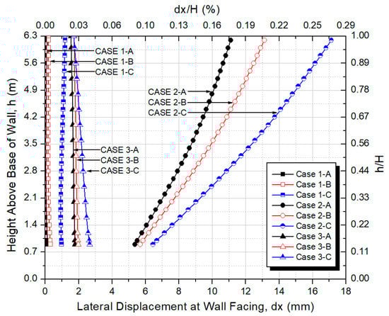
Figure 7.
Lateral displacements at the wall facing, dx (mm), when models are subjected to different static loadings: Case 1A, 2A, 3A (end of bridge construction); Case 1B, 2B, 3B (applied general traffic loading); and Case 1C, 2C, 3C (applied railway loading).
3.1.1. Effects of Wall Facing Type and Construction on Lateral Displacements at Wall Facing
In this study, the results show that the dx behaviors at the wall facing in each model are very distinct from each other. The differences may be attributed to the effects of having a different wall facing material, design, and construction method. Hence, Case 1A–C (GRS-IB) models showed the least dx at the wall facing compared to those of Case 2A–C (GRS-IBS) and Case 3A–C (IB) models (see Figure 7). This is because the GRS-IB technology allows the dx at the wall facing to occur during the construction. Afterwards, the GRS wall facing dx during the construction had been eliminated when the FHR facing was constructed. The negligible dx at the wall facing is due to the post-construction surcharge loads. This is one of the advantages of this technology wherein compaction can be applied thoroughly but cautiously on the backfill, especially near the wall facing, without too much concern for wall facing damage or excessive deformation. Moreover, the FHR facing of the GRS-IB model carries the loads from the reinforced concrete (RC) girder, hence, the GRS abutment carries the minimal surcharge loads. It can be observed that the dx behavior of the FHR facing did not bulge but was rather almost straight from the base towards the top of the wall. This may be because the FHR facing of the GRS-IB is 0.90 m thick and has very high stiffness. Thus, the dx at the wall facing of GRS-IB (Case 1A–C) models after the bridge construction and load application is very minimal, with a maximum range of 0.002–0.02% (dx/H) at the top of the wall facing.
In contrast, Case 2A–C (GRS-IBS) showed the highest dx at the wall facing compared to Case 1A–C (GRS-IB) and Case 3A–C (IB) models (see Figure 7). The dx at the wall facing in the GRS-IBS models after the bridge construction and load application is greater than those in the GRS-IB and IB models, with a maximum range of 0.18–0.27% (dx/H) at the top of the wall facing. This occurred because the GRS-IBS models have 0.50 m-thick concrete masonry blocks as the wall facing material, whereas the GRS-IB and IB models have 0.90 m-thick FHR facing. The GRS wall is a flexible structure and the wall facing is weak at the block-to-block joint connection. Thus, an outward movement of the block facing is expected to occur during the construction due to the lateral earth pressure from the backfill soil. In addition to that, the bridge surcharge loads are directly applied on the bridge seat at the top of the abutment and are supported by the geosynthetic-reinforced bearing zone. Hence, the greater dx at the wall facing occurred as a result of the increase in lateral earth pressures due to the additional bridge surcharge loads. Moreover, the deformation of the reinforced soil foundation (RSF) may have attributed also to the magnitude of the dx at the wall facing.
The last case models, Case 3A–C, exhibited similar dx behavior at the wall facing compared to Case 1A–C (GRS-IB) models but slightly greater (see Figure 7). The differences between the two bridge designs are that the IB models have no reinforcements in the backfill and have a wider RC footing that extends behind the wall facing. In this case, the construction and type of wall facing influenced the behavior of its dx. During construction, the IB FHR facing and RC footing were activated first before the backfill lifts had been placed. When the IB FHR facing and RC footing were constructed above the reinforced soil foundation (RSF), the RSF exhibited more displacements at the toe than at the heel, probably due to the distribution of the IB dead loads. At the end of the bridge construction, it is noticeable that dx at the wall facing is very minimal. This may be because the wall facing of the IB is 0.90 m thick and has a very high stiffness. It can be implied that the initial movement of the IB wall facing and footing at the start of the construction may have greatly affected the dx behavior showed by the IB models. Hence, the dx at the wall facing in the IB (Case 3A–C) models after the bridge construction and load application is very minimal, with a maximum range of 0.03–0.04% (dx/H) near the base of the wall facing.
Nevertheless, the dx at the wall facing in the GRS-IB (Case 1A–C), GRS-IBS (Case 2A–C), and IB (Case 3A–C) models are less than the maximum allowable lateral displacement of 1% (dx/H). The results inferred that the lateral displacement behavior at the wall facing depends on the type of wall facing system, wall construction method, backfill placement method, and reinforcement-wall facing connection details. In this study, the GRS-IB models performed best compared to the GRS-IBS and IB models.
3.1.2. Effects of Surcharge Loads on Lateral Displacements at the Wall Facing
The bridge and roadway approach backfill dead loads, general traffic loads, and railway loads are modelled as surcharge loads and applied uniformly on the top of the bridge abutment. In general, the dx at the wall facing increases as the surcharge load increases. The effects of the applied surcharge loads on the lateral displacement at the wall facing are shown in Figure 8. Here, the lateral displacement ratio is computed as , where is the lateral displacements at the wall facing for models that are subjected to general traffic loadings and railway loadings (Case 1B, 2B, 3B and Case 1C, 2C, 3C), and is the lateral displacements at the wall facing at the end of the bridge construction (Case 1A, 2A, 3A).
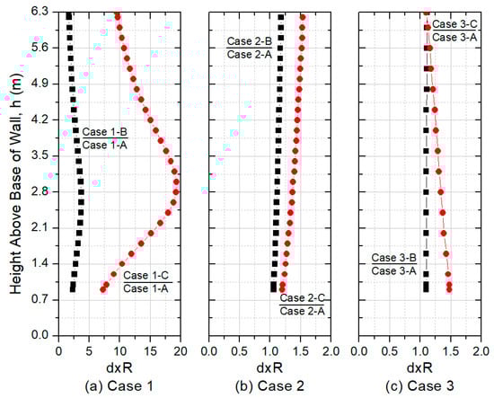
Figure 8.
Lateral displacement ratio, dxR, at the wall facing, showing the increase of dx after the applied surcharge loads.
The results plotted in Figure 8a show that Case 1B had a maximum increase of 3.7 times when the additional load of 30 kPa (traffic load) was applied on the bridge after the bridge construction and that Case 1C had a maximum increase of 19 times when the additional load of 50 kPa (railway load) was applied on the bridge after the bridge construction. Here, the effects of the applied loading for Case 1A–C are great at 2.80 m above the base of the wall. The magnitude of dxR for Case 1B–C may seem great because it is relative to the dx at the end of the bridge construction (Case 1A) which is almost zero (0.002% dx/H max) (refer to Figure 7). Conversely, the magnitudes of dxR are about similar for Case 2A–C, which are between 1.06 and 1.54 (Figure 8b), and Case 3A–C, which are between 1.10 and 1.48 (Figure 8c). However, the dxR trends are opposite. The effects of the applied loads for Case 2A–C are great at the top of the wall facing, while the effects of the applied loads for Case 3A–C are great at the base of the wall. The trends of dxR shown by the models are very similar to the dx behavior shown in Figure 7. Here, the magnitude of dxR are quite small because it is relative to the dx at the end of the bridge construction; consider Case 2A (0.18% dx/H max) and Case 3A (0.03% dx/H max), which are a lot higher than Case 1A (0.002% dx/H max).
3.2. Vertical Displacements at the Top of the Wall Abutment
3.2.1. Effects of the Wall Facing Type and Construction on Vertical Displacements at the Top of the Wall Abutment
The vertical displacements (dy) at the top of the wall abutment at the end of the bridge construction (Case 1A, 2A, 3A) after the applied general traffic loading (Case 1B, 2B, 3B) and railway loading (Case 1C, 2C, 3C) are shown in Figure 9. In the figure, the horizontal distanceS (x) from the wall facing from 0.90 m (for Case 1A–C and Case 3A–C) and 0.50 m (for Case 2A–C) until 7.8 m and 11.2 m are the reinforced zone and backfill soil zone, respectively. The horizontal distance (x) beyond 11.2 m from the wall facing is the retained soil zone where dy is the same from that point towards the end boundary at 22.5 m from the wall facing. The vertical displacements (dy) shown in the figures are carried over from the start of the construction until the end of the bridge construction, without any corrections; in other words, there is no reset of vertical displacements done in the Plaxis 2D staged construction mode.
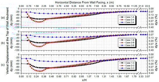
Figure 9.
Vertical displacements at the top of the wall abutment, dy (mm): (a) Case 1A, 2A 3A (end of bridge construction); (b) Case 1B, 2B, 3B (general traffic loading); and (c) Case 1C, 2C, 3C (railway loading).
The results show that the GRS-IB (Case 1A–C) models obtained the maximum dy of 65.72 mm, 70.95 mm, and 85.18 mm, located at 1.80 m, 1.95 m, and 2.40 m from the wall facing after the integral bridge construction (Case 1A), applied general traffic loading (Case 1B), and applied railway loading (Case 1C), respectively. Moreover, the GRS-IBS (Case 2A–C) models obtained the maximum dy of 84.26 mm, 95.32 mm, and 106.01 mm after the integral bridge construction (Case 2A), applied general traffic loading (Case 2B), and applied railway loading (Case 2C), respectively, located at 1.80 m from the wall facing. Lastly, the IB (Case 3A–C) models obtained the maximum dy of 31.09 mm, 34.57 mm, and 44.30 mm after the integral bridge construction (Case 3A), applied general traffic loading (Case 3B), and applied railway loading (Case 3C), respectively, located at 3.91 m and 4.31 m from the wall facing. Nevertheless, the dy at the top of the abutment in the GRS-IB (Case 1A–C), GRS-IBS (Case 2A–C), and IB (Case 3A–C) models are less than the allowable vertical displacement of 0.5% (dy/x). The GRS-IBS models exhibited the greatest vertical displacements compared to those of the GRS-IB and IB models, which are located at the bridge seat, specifically at 1.80 m from the wall facing. In addition, the results show that the GRS retaining wall abutment of the GRS-IB and GRS-IBS models exhibited greater vertical displacements than those of the unreinforced IB models. This may be attributed to the effects of the wall facing type and construction. Similar to the lateral displacement behavior at the wall facing, the type of wall facing and its construction also greatly affect the vertical displacement behavior of the models and the magnitude of the vertical displacements increases as the applied loading increases.
At this point, each bridge design shall be compared to better understand its corresponding vertical displacement behavior. First, we will discuss the GRS-IB versus IB models. The results show that the GRS-IB (Case 1A–C) models exhibited twice as much vertical displacements than those of the IB (Case 3A–C) models despite having the geosynthetic reinforcements. This is because during the construction of the GRS-IB models, the GRS wall abutment was constructed without the FHR facing. The gravel bags and geosynthetic-wrapped facing of Case 1A–C are flexible and as a results of the increasing lateral earth pressures during construction, the wall facing greatly moved outwards and exhibited more deformation than the FHR facing, thus inducing more dy in the backfill soil zone. The deformation increases in every placement of backfill lifts and are then collated until the end of the abutment construction. Then, the FHR facing in the GRS-IB models was constructed after the GRS wall abutment had been completed. Therefore, the facing deformation during the construction affects greatly the vertical displacement behavior of the GRS-IB models, in addition to the RSF and backfill soil deformation. However, in the IB models, the FHR facing was constructed before the backfill soil lifts were placed. Hence, the vertical displacements obtained by the IB models are less affected by the facing deformation but more by the RSF and backfill soil deformation. In addition, the results show that the maximum dy in the GRS-IB models are located within the first quarter of the reinforced zone or within 0.38 H from the wall facing, while in the IB models, the maximum dy are located near the first one-third of the backfill soil zone or 0.62 H from the wall facing.
Next, we discuss the GRS-IB versus GRS-IBS models. It is comparable that the GRS-IB (Case 1A–C) and GRS-IBS (Case 2A–C) models exhibited almost similar dy behavior at the top of the wall abutment because these models have geosynthetic reinforcements, although with few reasonable distinctions. The results show that the maximum dy in the GRS-IB models are located within 1.8 m to 2.4 m from the wall facing, while the maximum dy in the GRS-IBS models are located at 1.8 m from the wall facing. Both the GRS-IB and GRS-IBS models showed the maximum dy within the first quarter (0.25 L) to about one-third (0.34 L) of the reinforcement length (L). Hence, one of the few distinctions in the dy behavior of the GRS-IB and GRS-IBS models can be observed from 0.5 m to 2.5 m from the wall facing. This is because for the GRS-IBS model, the bridge loadings are applied directly on top of the bridge seat zone (0.75 m to 2.25 m from the wall facing), which are 2.2–5.6 times greater than the roadway loadings. Another distinction in the dy behavior can be observed at the wall facing. The GRS-IB models exhibited larger dy at the wall facing because the bridge loadings were supported by the 0.90 m-thick FHR facing, whereas the GRS-IBS models had 0.50 m-width block facing that did not carry any external vertical loads. Lastly, it can be observed that after 3.0 m from the wall facing, the GRS-IBS models showed lesser dy than those of the GRS-IB models. In this case, the dy behavior was influenced by the backfill soil deformation during the construction. The GRS-IB models have greater backfill zone deformation than those of the GRS-IBS models because the GRS-IB models have weaker wall facing, thus exhibiting greater wall facing deformation.
3.2.2. Vertical Displacement Increments at the Top of the Wall Abutment due to Applied Loadings
The main function of soil reinforcement is to restrain soil deformation. Hence, the effects of soil reinforcement can be observed in Figure 10. The figure shows the vertical displacement increments (∆dy) obtained from the current calculation phase for (a) the applied general traffic loads (Case 1B, 2B, 3B) and (b) applied railway loads (Case 1C, 2C 3C).
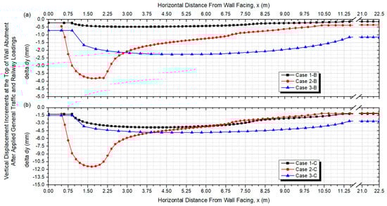
Figure 10.
Vertical displacement increments at the top of the wall abutment, ∆dy (mm), after the applied static loadings: (a) Case 1B, 2B 3B (general traffic loading) and (b) Case 1C, 2C, 3C (railway loading).
In this condition, the geosynthetic reinforcements worked well in the backfill soil by resisting the ∆dy from the vertical earth pressures induced by the applied surcharge loads. The results in Figure 10a,b show that the GRS-IB models with FHR facing and reinforced backfill exhibited the least vertical displacement increments (∆dy) at the top of the wall abutment. In this study, both the GRS-IB and IB models have the same loading conditions. Due to the presence of the reinforcements, the GRS-IB models have reduced the ∆dy by 4.7 times and 1.3 times (maximum) after the applied general traffic loads and railway loads compared to the IB models, respectively. Moreover, both the GRS-IB and GRS-IBS models use geosynthetic reinforcements. Yet, the GRS-IB models have reduced the ∆dy by eight times and three times (maximum) after the applied general traffic loads and railway loads, respectively. This is because for GRS-IBS models, the bridge loads are supported by the reinforced bridge seat in the abutment (0.75 m to 2.25 m from the wall facing), while for GRS-IB models, bridge loads are supported by the 0.90 m-thick FHR facing.
3.3. Lateral Stresses behind the Wall Facing
The lateral stresses or earth pressures behind the wall facing at the end of the bridge construction (Case 1A, 2A, 3A) after the applied general traffic loading (Case 1B, 2B, 3B) and applied railway loading (Case 1C, 2C, 3C) are presented in Figure 11a–c. In the figure, the lateral earth pressures behind the wall facing from 0.90 m above the base up to the top of the abutment have been considered to eliminate the part of the integral bridge footing (Case 1 and Case 3). The lateral earth pressures are the closest polynomial fit of the lateral Cartesian total stresses obtained from the Plaxis 2D output and are plotted alongside with the theoretical values of the at-rest earth pressures ( condition), Rankine’s active earth pressures ( condition), and lateral earth pressures for Case 2 with strip (bridge) loading. The at-rest and active lateral earth pressures were computed using the formulas and [], where is the roadway and approach backfill surcharge loads (Case 1A, 2A, 3A = 18 kPa; Case 1B, 2B, 3B = 30 kPa; and Case 1C, 2C, 3C = 68 kPa); the backfill soil unit weight is γ = 19 kN/m3; the coefficient of earth pressure at-rest () was assumed as 0.50 in the initial condition of the Plaxis 2D simulation; and the coefficient of the active earth pressure () was computed using Rankine’s formula, , where φ = 51°, and the cohesion in this case was not considered, thus ( = 0) and = 0.1254.
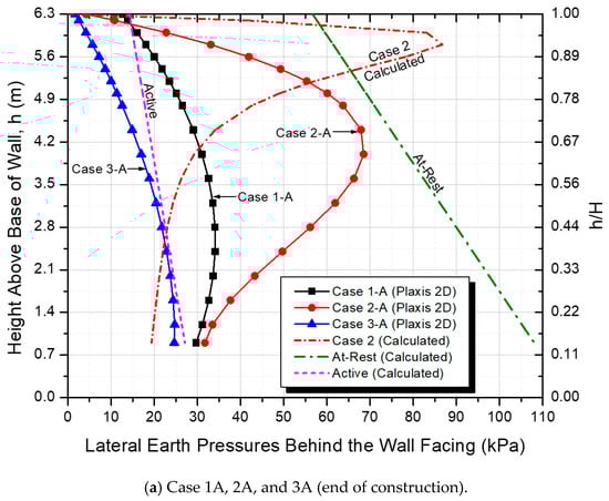
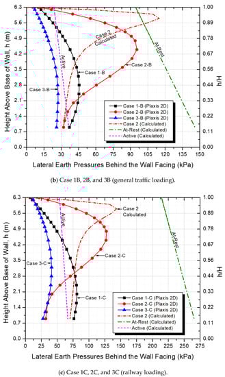
Figure 11.
Lateral earth pressures behind the wall facing at: (a) Case 1A, 2A, and 3A (end of construction); (b) Case 1B, 2B, and 3B (general traffic loading); and (c) Case 1C, 2C, and 3C (railway loading).
In this study, Case 2A–C (GRS-IBS) models have different loading conditions because the bridge surcharge loads are directly supported by the reinforced bridge seat located at 0.75 m to 2.25 m from the wall facing. The bridge loads are taken as strip loads on top of the rigid wall. The theoretical values of the lateral earth pressures on the GRS retaining wall, due to strip load, are computed based on the Boussinesq theory, [], where and in radians. The is the bridge surcharge loads (Case 2A = 100 kPa; Case 2B = 130 kPa; and Case 2C = 150 kPa); is the distance from the wall facing to the first point of the bridge surcharge load; is the distance from the wall facing to the end point of the bridge surcharge load; and is the vertical distance from the top of the wall. Hence, in comparing the theoretical and numerical results of the lateral earth pressures, the values are not in good agreement, yet the trends are slightly similar. Generally, the maximum lateral earth pressures for Case 2A–C based on the Plaxis 2D results are found below the bearing zone with a height from 4.0 m (0.63 H) to 4.8 m (0.76 H) above the base of the wall, whereas the maximum lateral earth pressures for Case 2A~C based on the form of the theoretical values are found at 5.80 m (0.92 H) above the base of the wall. The deviations may be attributed to the presence of the geosynthetic reinforcements at the bearing zone (under the bridge seat) between heights 4.8 m (0.76 H) to 6.3 m (H). Moreover, the lateral earth pressure trends of Case 2A–C are reasonably different from those of Case 1A–C and Case 3A–C due to the strip load. The results in Figure 11a–c show that the Case 2A–C models exhibited the largest lateral earth pressures, which are in agreement with its corresponding lateral displacement (dx) behavior at the wall facing (refer also to Figure 7).
Additionally, the results showed that the Case 3A–C (IB) models have lesser lateral earth pressure than those of the Case 1A–C (GRS-IBS) models, despite the latter having lesser lateral displacements at the wall facing than the former. Although the displacements at the wall facing have been reset during the numerical simulation of Case 1A–C at the end of the bridge construction, the pressures are still carried over from the beginning until the end of construction.
In general, based on the results shown in Figure 11, the lateral earth pressures behind the wall facing increase as the general traffic and railway loads are applied after the bridge construction. After the bridge construction, the lateral earth pressures increase by 1–34% (Case 1B), 1–162% (Case 2B), and 5–255% (Case 3B) when the general traffic loadings were applied. Similarly, the lateral earth pressures increase by 9–157% (Case 1C), 1–407% (Case 2C), and 12–515% (Case 3C) when the railway loadings were applied after the bridge construction. The lateral earth pressures of the Case 3A–C numerical models are less than the Rankine active earth pressures, while the lateral earth pressures of the Case 1A–C and Case 2A–C numerical models are generally larger than the Rankine active earth pressures but less than the at-rest earth pressure. Moreover, the results show that none of the models are in good agreement with the active condition as well as the at-rest condition. Wu [] introduced the so-called bin pressure, wherein the lateral earth pressures are confined within each layer of reinforcement in the GRS walls, therefore lateral earth pressure on the face does not increase with depth. The lateral earth pressure is practically not dependent on the GRS wall height but is mainly dependent on the spacing of reinforcement.
3.4. GRS Wall Potential Failure Surfaces and Reinforcement Behavior
3.4.1. Location of Potential Failure Surfaces in the GRS Wall
The potential failure surface in a reinforced soil wall is assumed to coincide with the locus of the maximum tensile force in each reinforcement layer []. The locus of the maximum tensile force in each reinforcement layer concurs with the locus of the maximum strain, wherein the potential failure surface may occur. Hence, in this study, Figure 12 shows the locations of the maximum reinforcement strain obtained from the numerical analysis results with height of the wall and the theoretical potential failure surfaces for comparison. It can be observed that the locus of maximum reinforcement strain is generally within the active zone, within the theoretical zone of the maximum stress, or on thr potential failure surface for extensible reinforcements. Moreover, it can be observed that from the 7th reinforcement layer ( m), going down towards the base of the wall, the maximum reinforcement strains are found outside the theoretical active zone for both the GRS-IB and GRS-IBS models. The presence of the foundation soil at the bottom front of the wall facing may have attributed to the deviation of the maximum reinforcement strain location at the lower reinforcement layers due to the lateral pressures that it created.
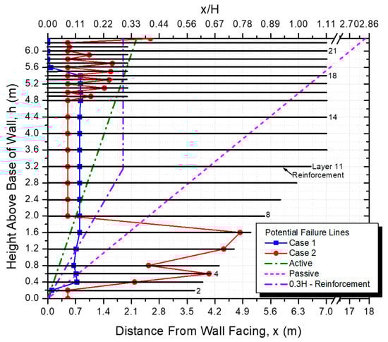
Figure 12.
Locus of maximum reinforcement strain and potential failure surface.
3.4.2. Reinforcement Behavior
When the failure develops, the geosynthetic (extensible) reinforcement tends to elongate and may be deformed at the point at which it intersects with the failure surface. This results in an increase of tensile force in the reinforcement []. In this study, the distribution of reinforcement forces at seven elevations (seven reinforcement layers) within the GRS abutment are plotted in Figure 13 and Figure 14 for the GRS-IB (Case 1) and GRS-IBS (Case 2) models, respectively. The seven elevations that correspond to the reinforcement layer numbers 2, 4, 8, 11, 14, 18, and 21 are taken into consideration because of its significant behavior as observed from Figure 12. There are several points of comparison between the Case 1 and Case 2 reinforcement behavior as shown in Figure 13 and Figure 14, respectively. The results show that the reinforcements in Case 2 exhibited greater forces than those in Case 1. This can be attributed to the great bridge surcharge loads that is directly supported by the Case 2 GRS abutment at the bearing bed (bridge seat). Hence, it can be observed that upper reinforcement layers exhibited greater forces than those at lower layers. On the contrary, the lower reinforcement layers for Case 1 exhibited greater forces than those at the upper layers. Moreover, the maximum reinforcement forces in Case 1 occurred mostly at 0.80 m from the wall facing, while the maximum reinforcement forces in Case 2 occurred mostly at the connection point of the reinforcement and block facing, which is 0.5 m from the wall facing. It can be inferred that the connection point of the block facing and reinforcement at 0.50 m from the wall facing is critical. The difference in stiffness and unit weight between the block and backfill soil may have attributed to behavior of the reinforcement at the said connection point. Consequently, the differences in settlement between the block facing and backfill soil, which are evident at the top and base of the wall, resulted in an increase of reinforcement forces or strain at the said connection point. Lastly, both models also exhibited great tension near the end of the reinforcements, which indicates the limiting shear stress for pullout.
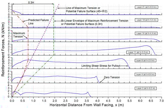
Figure 13.
Distribution of reinforcement forces at seven elevations within the GRS abutment for Case 1.
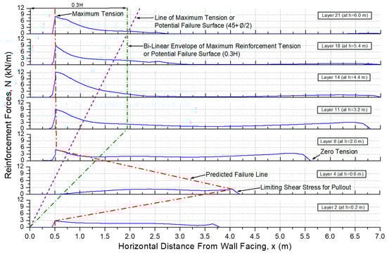
Figure 14.
Distribution of reinforcement forces at seven elevations within the GRS abutment for Case 2.
4. Numerical Analysis Results and Discussion under Dynamic Loading
The results on the seismic response of the finite element (FE) models at a certain point on the top of the wall abutment are shown in Figure 15. It can be observed that the numerical models naturally show a vibration decay even without the applied damping. Generally, the total displacement curves straighten at the point after 0.75 s of the dynamic time.
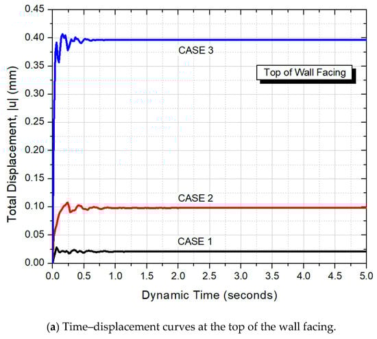
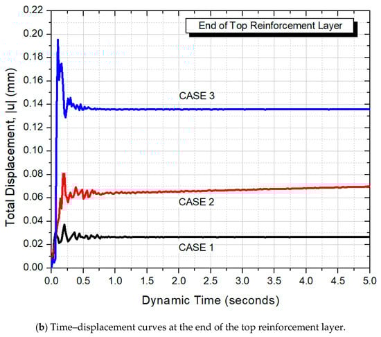
Figure 15.
Time-displacement curves at the top of the wall due to seismic load.
For the seismic response at the top of the wall facing (see Figure 15a), the vibrations are intense between the periods of 0 s to 0.5 s. Moreover, the results show that the Case 1 (GRS-IB) model has the least total displacement in response to the seismic loading, followed by the Case 2 (GRS-IBS) model and Case 3 (IB) model which showed the greatest total displacement in response to the seismic loading. Similarly, the seismic response at the end of the top reinforcement layer (see Figure 15b) showed that, generally, the total displacement curves straighten at the point after 0.75 s of the dynamic time. In this case, the vibrations are more intense between the periods of 0 s to 0.75 s but have a lesser magnitude compared to those at the wall facing. Moreover, the results show that the Case 1 (GRS-IB) model has the least total displacement in response to the seismic loading, followed by the Case 2 (GRS-IBS) model and Case 3 (IB) model which showed the greatest total displacement in response to the seismic loading.
5. Conclusions
In this study, there are three types of bridges that are designed, modelled, and analyzed using the finite element (FE) method in Plaxis 2D. The analyses and comparison of the behavior of each model after being subjected to static and dynamic loadings are presented in this paper. The main conclusions drawn from the series of numerical analysis are as follows:
- Generally, the numerical results showed that the GRS-IB technology performed better than the GRS-IBS and IB technologies considering the internal and external behavior of the numerical models when subjected to static and dynamic loads.
- The GRS-IB numerical models exhibited satisfactory and stable behavior when subjected to static and dynamic loads.
Therefore, the results of this study suggest that GRS-IB is a remarkable technology with great performance when subjected to static and dynamic loads. Thus, this technology is worth recommending for application in the Philippines, with confidence that it can withstand extreme magnitudes of earthquakes, along with other advantages.
Author Contributions
Conceptualization, M.-S.W. and C.P.L.; methodology, M.-S.W. and C.P.L.; software, C.P.L.; validation, M.-S.W. and C.P.L.; formal analysis, M.-S.W. and C.P.L.; investigation, C.P.L.; resources, M.-S.W.; data curation, C.P.L.; writing—original draft preparation, C.P.L.; writing—review and editing, M.-S.W. and C.P.L.; visualization, C.P.L.; supervision, M.-S.W.; project administration, M.-S.W.; funding acquisition, M.-S.W. All authors have read and agreed to the published version of the manuscript.
Funding
This study was supported by the Basic Science Research Program through the National Research Foundation of Korea (NRF), funded by the Ministry of Education (NRF2021R1A6A1A0304518511).
Institutional Review Board Statement
Not applicable.
Informed Consent Statement
Not applicable.
Data Availability Statement
The data presented in this study are available on request from the corresponding author.
Conflicts of Interest
The authors declare no conflict of interest. The funders had no role in the design of the study; in the collection, analyses, or interpretation of data; in the writing of the manuscript, or in the decision to publish the results.
References
- Adams, M.; Nicks, J.; Stabile, T.; Wu, J.; Schlatter, W.; Hartmann, J. Geosynthetic Reinforced Soil Integrated Bridge System, Synthesis Report (FHWA-HRT-11-027); Federal Highway Administration U.S. Department of Transportation: Washington, DC, USA, 2011.
- Holtz, R.D. 46th Terzaghi lecture: Geosynthetic reinforced soil: From the experimental to the familiar. J. Geotech. Geoenviron. Eng. 2017, 143, 03117001. [Google Scholar] [CrossRef]
- Jones, C.J.F.P. Earth Reinforcement and Soil Structures; Butterworth’s Advanced Series in Geotechnical Engineering; Butterworth-Heinemann: Oxford, UK, 1985. [Google Scholar]
- Berg, R.R.; Christopher, B.R.; Samtani, N.C. Design of Mechanically Stabilized Earth Walls and Reinforced Soil Slopes; Volume I (FHWA-NHI-10-024 FHWA GEC 011-Vol I); National Highway Institute, Federal Highway Administration, U.S. Department of Transportation: Washington, DC, USA, 2009.
- Koerner, R.M.; Koerner, G.R. The importance of drainage control for geosynthetic reinforced mechanically stabilized earth walls. J. GeoEng. 2011, 6, 3–13. [Google Scholar]
- Koerner, R.M.; Koerner, G.R. A data base, statistics and recommendations regarding 171 failed geosynthetic reinforced mechanically stabilized earth (MSE) walls. Geotext. Geomembr. 2013, 40, 20–27. [Google Scholar] [CrossRef]
- Shin, E.C.; Cho, S.D.; Lee, K.W. Case study of reinforced earth wall failure during extreme rainfall. In Proceedings of the TC 302 Symposium: International Symposium on Backward Problems in Geotechnical Engineering and Monitoring of Geo-Construction, Osaka, Japan, 14–15 July 2011; pp. 146–153. [Google Scholar]
- Adams, M.; Nicks, J.; Stabile, T.; Wu, J.; Schlatter, W.; Hartmann, J. Geosynthetic Reinforced Soil Integrated Bridge System Interim Implementation Guide (FHWA-HRT-11-026); Federal Highway Administration U.S. Department of Transportation: Washington, DC, USA, 2012.
- Tatsuoka, F.; Tateyama, M.; Koda, M.; Kojima, K.; Yonezawa, T.; Shindo, Y.; Amai, S. Recent research and practice of GRS integral bridges for railways in Japan. Jpn. Geotech. Soc. Spec. Publ. 2016, 2, 2307–2312. [Google Scholar] [CrossRef] [Green Version]
- Tatsuoka, F.; Tateyama, M.; Koseki, J.; Yonezawa, T. Geosynthetic-reinforced soil structures for railways in Japan. Transp. Infrastruct. Geotechnol. 2014, 1, 3–53. [Google Scholar] [CrossRef] [Green Version]
- Tatsuoka, F.; Tateyama, M.; Mohri, Y.; Matsushima, K. Remedial treatment of soil structures using geosynthetics-reinforcing technology. Geotext. Geomembr. 2007, 25, 204–220. [Google Scholar] [CrossRef]
- Tatsuoka, F.; Tateyama, M.; Uchimura, T.; Koseki, J. Geosynthetic-reinforced soil retaining walls as important permanent structures. Geosynth. Int. 1997, 4, 81–136. [Google Scholar] [CrossRef]
- Koda, M.; Nonaka, T.; Suga, M.; Kuriyama, M.; Tateyama, M.; Tatsuoka, F. A Series of Lateral Loading Tests on a Full-Scale Model of Geosynthetic-Reinforced Soil Integral Bridge. In Proceedings of the International Symposium on Design and Practice of Geosynthetic-Reinforced Soil Structures, Bologna, Italy, 11–16 October 2013; pp. 157–174. [Google Scholar]
- Yazaki, S.; Tatsuoka, F.; Tateyama, M.; Koda, M.; Watanabe, K.; Duttine, A. Seismic design of GRS integral bridge. In Proceedings of the International Symposium on Design and Practice of Geosynthetic-Reinforced Soil Structures, Bologna, Italy, 11–16 October 2013; pp. 142–156. [Google Scholar]
- Ardah, A.; Abu-Farsakh, M.; Voyiadjis, G. Numerical evaluation of the performance of a Geosynthetic Reinforced Soil-Integrated Bridge System (GRS-IBS) under different loading conditions. Geotext. Geomembr. 2017, 45, 558–569. [Google Scholar] [CrossRef]
- Lenart, S.; Kralj, M.; Medved, S.P.; Suler, J. Design and construction of the first GRS integrated bridge with FHR facings in Europe. Transp. Geotech. 2016, 8, 26–34. [Google Scholar] [CrossRef]
- Das, B.M. Principles of Foundation Engineering, 7th ed.; Cengage Learning: Stamford, CT, USA, 2012. [Google Scholar]
- Murthy, V.N.S. Geotechnical Engineering: Principles and Practices of Soil Mechanics and Foundation Engineering; CRC Press: Boca Raton, FL, USA, 2002. [Google Scholar]
- Abu-Farsakh, M.; Ardah, A.; Voyiadjis, G. 3D Finite element analysis of the geosynthetic reinforced soil-integrated bridge system (GRS-IBS) under different loading conditions. Transp. Geotech. 2018, 15, 70–83. [Google Scholar] [CrossRef]
- Abu-Farsakh, M.; Ardah, A.; Voyiadjis, G. Numerical parametric study to evaluate the performance of a Geosynthetic Reinforced Soil–Integrated Bridge System (GRS-IBS) under service loading. Transp. Geotech. 2019, 20, 100238. [Google Scholar] [CrossRef]
- Ardah, A.; Abu-Farsakh, M.; Voyiadjis, G. Numerical parametric study of geosynthetic reinforced soil integrated bridge system (GRS-IBS). Geotext. Geomembr. 2021, 49, 289–303. [Google Scholar] [CrossRef]
- Zheng, Y.; Fox, P.J. Numerical investigation of the geosynthetic reinforced soil–integrated bridge system under static loading. J. Geotech. Geoenviron. Eng. 2017, 143, 04017008. [Google Scholar] [CrossRef]
- Plaxis BV. Plaxis 2D Reference Manual; Plaxis B.V.: Delft, The Netherlands, 2018. [Google Scholar]
- Plaxis BV. Plaxis 2D Tutorial Manual; Plaxis B.V.: Delft, The Netherlands, 2018. [Google Scholar]
- Damians, I.P.; Bathurst, R.J.; Josa, A.; Lloret, A.; Albuquerque, P.J.R. Vertical facing loads in steel reinforced soil walls. J. Geotech. Geoenviron. Eng. 2013, 139, 1419–1432. [Google Scholar] [CrossRef]
- Damians, I.P.; Bathurst, R.J.; Josa, A.; Lloret, A. Numerical analysis of an instrumented steel-reinforced soil wall. Int. J. Geomech. 2015, 15, 1–15. [Google Scholar] [CrossRef]
- Damians, I.P.; Bathurst, R.J.; Lloret, A.; Josa, A. Vertical facing panel-joint gap analysis for steel-reinforced soil walls. Int. J. Geomech. 2016, 16, 04015103. [Google Scholar] [CrossRef] [Green Version]
- Yu, Y.; Bathurst, R.J.; Allen, T.M.; Nelson, R. Physical and numerical modelling of a geogrid reinforced incremental concrete panel retaining wall. Can. Geotech. J. 2016, 53, 1883–1901. [Google Scholar] [CrossRef]
- Yu, Y.; Bathurst, R.J. Influence of selection of soil and interface properties on numerical results of two soil geosynthetic interaction problems. Int. J. Geomech. 2017, 17, 04016136. [Google Scholar] [CrossRef]
- Yu, Y.; Bathurst, R.J.; Miyata, Y. Numerical analysis of mechanically stabilized earth wall reinforced with steel strips. Soils Found. 2015, 55, 536–547. [Google Scholar] [CrossRef]
- Visone, C.; Santucci de Magistris, F. Some Aspects of Seismic Design Methods for Flexible Earth Retaining Structures. Workshop of ERTC12–Evaluation Committee for the Application of EC8 Special Session XIV ECSMGE, Madrid, Patron Ed., Bologna. 2007. Available online: http://www.reluis.it/doc/pdf/Pubblicazioni/vissao.pdf (accessed on 8 April 2021).
- Wu, J.T.H. Lateral earth pressure against the facing of segmental GRS walls. In Geosynthetics in Reinforcement and Hydraulic Applications (GSP 165); Gabr, B., Ed.; ASCE: Reston, VA, USA, 2007; pp. 165–175. [Google Scholar]
Publisher’s Note: MDPI stays neutral with regard to jurisdictional claims in published maps and institutional affiliations. |
© 2021 by the authors. Licensee MDPI, Basel, Switzerland. This article is an open access article distributed under the terms and conditions of the Creative Commons Attribution (CC BY) license (https://creativecommons.org/licenses/by/4.0/).