Article

Model Predictive Control for Flexible Job Shop Scheduling in Industry 4.0 †

by
Philipp Wenzelburger
* and
Frank Allgöwer
Institute for Systems Theory and Automatic Control (IST), University of Stuttgart, Pfaffenwaldring 9, 70569 Stuttgart, Germany
*
Author to whom correspondence should be addressed.
This paper is an extended version of two of our conference papers.
Appl. Sci. 2021, 11(17), 8145; https://doi.org/10.3390/app11178145
Submission received: 23 July 2021 / Revised: 25 August 2021 / Accepted: 27 August 2021 / Published: 2 September 2021
(This article belongs to the Special Issue Planning and Scheduling of Manufacturing Systems)

Abstract

:
In the context of Industry 4.0, flexible manufacturing systems play an important role. They are designed to provide the possibility to adapt the production process by reacting to changes and enabling customer specific products. The versatility of such manufacturing systems, however, also needs to be exploited by advanced control strategies. To this end, we present a novel scheduling scheme that is able to flexibly react to changes in the manufacturing system by means of Model Predictive Control (MPC). To introduce flexibility from the start, the initial scheduling problem, which is very general and covers a variety of special cases, is formulated in a modular way. This modularity is then preserved during an automatic transformation into a Petri Net formulation, which constitutes the basis for the two presented MPC schemes. We prove that both schemes are guaranteed to complete the production problem in closed loop when reasonable assumptions are fulfilled. The advantages of the presented control framework for flexible manufacturing systems are that it covers a wide variety of scheduling problems, that it is able to exploit the available flexibility of the manufacturing system, and that it allows to prove the completion of the production problem.

1. Introduction

In the prospect of smart factories, industrial manufacturing is in the middle of an evolution that heads towards increasingly interconnected and digitized production systems. New paradigms evolve which make use of novel technologies from the field of information and communication technology, and their potential is exploited in an effort which is recognized as fourth industrial revolution (Industry 4.0) [1]. This trend is fostered by increased computational power, ongoing miniaturization of computational units, as well as faster and more reliable communication system. Previously purely mechanical machines are equipped with sensors, computational units, and communication interfaces, which enables decentralized reasoning, decision-making, and integration in an interconnected production system, rendering the machines into a cyber-physical production system (CPPSs) that can interact with their environment physically as well as via digital communication [2]. This allows to have instantaneous feedback from the production process which is provided to a digital decision making and scheduling system. Such information can be exploited to react to problems in the production process, perform real-time optimization, and even predict imminent failures and act before they occur [3].
The development on the digital side goes hand in hand with a change from rigid production lines to flexible manufacturing systems (FMSs). This development is driven by a more diverse customer demand ranging towards individualized products and has the goal of enabling the manufacturing of products in lot size one at the cost of mass production [1,4]. The focus of industrial production changes from highly automated mass production to more adaptable manufacturing processes. This requires truly flexible manufacturing systems that are capable of changing according to the present needs. On the one hand, the physical manufacturing units need to be flexible, and on the other hand, also their control and their integration in the overall process require the capability to adapt in order to handle manufacturing orders of different types.
To manage the flexible manufacturing units, the concept of the digital twin is introduced. It describes the notion of having a real-time synchronized virtual equivalent of the real world objects in a digital environment that can be used in the decision-making process [3,5]. The organization of the production, the manufacturing units, and the parts being produced is coordinated digitally by means of their digital twins, which comprises their current status, their abilities, and a digital documentation of their past. The up-to-date status information and the knowledge about the capabilities of the physical system represented in its digital twin allow for digital panning and control and are the prerequisite to formulate the online optimization problem introduced in Section 4.1.
A very promising approach to exploit these information is the concept of skill-based programming, where commands to a robot or machine are abstracted to a higher level [6,7]. It became popular in the field of robot programming, where the high level of abstraction is provided to the user in order to simplify the usage of versatile robots [8,9,10,11,12,13]. On the high abstraction level, the operator can access the skills of the machines and give the desired instructions, which are passed to the machines that interpret and execute the incoming commands according to their capabilities by means of a subordinate logic. This approach enables the flexible use of versatile manufacturing units in complex production scenarios. Although it was initially conceived for easy human machine interaction, it also facilitates the automated interconnection of manufacturing units on the higher abstraction level.
The goal of a factory designed according to Industry 4.0 principles is to achieve a real-time optimal execution of the production process respecting the varying demand for diverse products. The optimization of the production could be done with regards to different criteria as for example work in progress or production time, but the economic goal to generate the maximum monetary profit remains the objective of every commercial production system. In order to achieve this goal, we aim to contribute to this development with control theoretic methods, building up on existing notions and results. In particular, we focus on the dynamic scheduling of customer specific orders in an FMS.
We take the concept of the digital twin as proposed by Grieves [5] as basis for our work and assume that the information on every physical system are always available in the corresponding digital twin and therefore can be used for the digital control of the manufacturing system. For a manufacturing unit, the digital twin particularly holds the manufacturing skills it can perform. Furthermore, a digital twin is initialized for every order that is placed at the manufacturing system. In this case, especially the production plan holding the necessary production steps for the requested product is of interest for our approach. The assignment between orders and manufacturing units is done based on their digital twins. On the one hand, the digital twin of the production orders requires skills of the manufacturing system for being produced and on the other hand, the manufacturing units offer those necessary skills. We formulate this assignment problem between required skills to produce the orders and available skills in the FMS as a scheduling problem.
The solution of the proposed scheduling problem is done on the basis of a Petri Net (PN) model, which is generated automatically from the initial description of the scheduling problem. The generation algorithms exploit the modular formulation of the initial scheduling problem, where the manufacturing units and the production orders can be considered as separate modules, and transforms it into a well-structured PN. The PN offers an algebraic representation that is used to determine the schedule for the FMS.
The result of the scheduling scheme are manufacturing decisions that are intended to be directly applied to the system in real-time. In order to exploit the flexibility of the FMS, it is important to keep the scheduling scheme flexible as well. Therefore, it is formulated in the form of a feedback control law, more precisely in the form of Model Predictive Control (MPC) [14]. MPC has the advantage that an optimization problem, in which the economic objective of the FMS can be considered, is solved while computing the scheduling inputs. The feedback mechanism of the MPC allows to immediately react to changes in the manufacturing system and to adjust its behavior accordingly.
The remainder of the paper is structured as follows. The description that we use for the scheduling problem will be further described in Section 2. It is kept in a rather general way such that it can be used for various specific cases. It is a generalization of the widely discussed job shop problem (JS) [15] and allows more general production plans with respect to the JS. This general form of a scheduling problem has, for example, practical applications in printing shops [16], and it can also be used to describe several special cases and practical applications thereof. A detailed description of the presented scheduling problem together with a classification with respect to a common classification scheme and a comparison with more common scheduling problems in literature can be found in Section 2. In this regard, we especially set the focus on the flexibility of the employed problem description.
In Section 3, we describe the automatic generation of a PN for the considered class of FMSs, which is used as mathematical basis to solve the scheduling problem. In this context, we slightly extend the classical notion of a PN in order to distinguish between autonomously running production processes and conscious production decisions. The generation process is discussed and the resulting PN is analyzed with respect to its relevant properties for the scheduling of the FMS.
Finally, two MPC schemes are introduced in Section 4, which determine the optimal scheduling decisions at the current time step with respect to a given cost function. We relate the presented approach to common control strategies for manufacturing and for PNs from literature. Most importantly, we provide proven guarantees of the MPC schemes that assure the completion of the scheduling problem based on a few natural assumptions.
In Section 5, we apply one of the presented MPC schemes in the simulation of two scheduling problems from literature. The results show that decent closed loop performance is achieved.
Section 6 summarizes and discusses the results with respect to the initially formulated objectives. It is explained how the results from Section 4 can be used in order to implement a suitable MPC formulation for a given manufacturing problem. The flexibility of the proposed solution is laid out and possible changes in the problem description are analyzed with respect to their effects on the MPC schemes. Further research opportunities are identified that enhance the presented methods. In Section 7, we draw a brief conclusion of our work.
The paper at hand is an extension of our conference papers [17,18] and repeats previous results in some indicated it paragraphs. Besides many additional explanations and bringing those two related works in their mutual context, our previous work is extended in various ways. On the level of the scheduling problem, this paper adds a more profound classification of the considered problem and describes its properties in a clearer form. For the automatically generated PN description, proofs of some important properties are provided. On the level of the MPC, the previously rather short proof of the main theorem is extended and now provides detailed descriptions of parts that were initially kept short due to page limitations. Additionally, a new MPC formulation is provided that significantly reduces the complexity of the employed optimization problem. Two simulation examples are added to show the applicability of our results with problem setups from literature.

2. Problem Description

The scheduling problem considered in this paper was originally proposed in our previous work [17] and describes an FMS with a given set of manufacturing units in which customer specific orders are fulfilled. It is a general case of the flexible job shop (FJS), which is further discussed in Section 2.3. Every customer specific order constitutes a specific and possibly unique job in the manufacturing system.
In order to arrive at a versatile modeling and control framework, we start from a very abstract description of the manufacturing problem which can be refined to describe several more specific scenarios. We want to exploit the flexibility to combine the skills of the available manufacturing units in the sense of skill based programming [6], in order to create and describe production plans. Therefore, our modeling approach has the skills as a central element. The manufacturing units have the skills to execute tasks, which are the basic building blocks for the jobs that have to be fulfilled by the manufacturing system. A job is completed once all its tasks have been completed. In a more formal way, the basic elements of the manufacturing problem are
  • a set T = { τ 1 , , τ n τ } of tasks that can be executed in the manufacturing system,
  • a set M = { M 1 , , M n M } of manufacturing units (robots, machines, automated guided vehicles,  etc.) which are called machines for brevity in the rest of this paper; every machine M can only execute a subset of tasks, which is specified as T M T ,
  • a set J = { J 1 , , J n J } of jobs that need to be fulfilled by the manufacturing system; every job J consists of a set T J T of tasks.
The purpose of the manufacturing system is to complete the jobs J J with the available machine pool M . The assignment between jobs and machines is done based on the tasks, which are the linking element between them. As different jobs J and J , which represent the instructions for the production of different goods, may share the same production steps, their sets T J and T J may contain the same elements. If we refer to a task τ T J of a specific job J, the pair ( τ , J ) of task and job is called operation O = ( τ , J ) . With this, the set of operations O is defined as O = { ( τ , J ) | τ T J } ( T × J ) . The term operation is mainly used to abbreviate certain statements, but in many cases we rather refer to the pair of task and job for the sake of clarity.
In the same way different jobs might share the same tasks, also different machines M and M might be able to execute the same tasks and hence the corresponding sets T M and T M may have elements in common. In this case and when considering the framework of skill-based programming [6], the fact that both machines can execute the same task does not mean that they do it in the same way. The machines might be of a different kind and it is not even necessarily required that the machines have some specific tool, as the introduction of a multipurpose machine by Brucker [15] suggests. In the framework of skill based programming [6], different production times for the same task might even result form different implementations of the same task or skill on different machines. For example, the tightening of a screw can be done with a tool that can rotate infinitely, or with a robotic arm that can only rotate by a limited angle and therefore needs to turn back and forth several times needing more time for a task that requires to tighten a screw. The skill to execute a task can be seen in the most abstract and general way possible. As the way in which a task is executed may vary from machine to machine, the production time t P ( M , τ ) R > 0 describing the amount of time that machine M needs to execute task τ not only depends on the task but also on the machine. The production times t P ( M , τ ) are assumed to be known and fixed for every valid combination of machine and task.
The general setup described above already contains several restrictions by itself and offers a variety of different flexibilities. A more detailed and structured description thereof is provided in the next section.

2.1. Restrictions and Flexibility in the Scheduling Problem

In the considered scheduling problem, there are restrictions concerning the three basic elements, i.e., tasks, machines, and jobs. To begin with, the sequence of tasks in a job is generally free. However, as there might be dependencies between the different steps in the production process of a product, these dependencies needs to be considered in the manufacturing problem such that only production sequences are scheduled which can be executed in the real production process. This is achieved through the following four restrictions in the scheduling problem related to the tasks:
(R1)
A task τ might not be independent, but require all tasks τ T τ in the set of its required tasks T τ T to be finished before it can be started.
(R2)
A task τ T J in a job J can only depend on tasks τ T J in the same job J, i.e.,  T τ T J for every task τ T J . If a task τ depends on another task τ , i.e.,  τ T τ , τ T J , then the operations O = ( τ , J ) and O = ( τ , J ) exist and it is said that O depends O . Operations O = ( τ , J ) and O ¯ = ( τ , J ¯ ) in different jobs J and J ¯ are independent from one another.
(R3)
Two tasks τ and τ must not be mutually dependent.
(R4)
Preemption of tasks is not allowed, i.e., once a task has been started it must be completed without interruption.
The restriction to a non-preemptive setup is the general case in literature and therefore adopted in the considered problem [19,20,21,22,23]. In the description of the dependencies of a task τ on other tasks (R1), only direct dependencies are provided in the sets T τ . Indirect dependencies with one or more other tasks in between can be recursively determined with an algorithm presented in our previous work [17]. The set of all tasks on which a task τ depends directly or indirectly is denoted with T ¯ τ . From the different sets T τ of the tasks τ T J of a job J, a precedence graph G J = ( T J , E J ) can be generated to represent the relations between the tasks of the job by considering the tasks τ T J as nodes and constructing the directed edges E J = { ( τ , τ ) | τ T τ , τ T J } according to the precedence relations in the sets T τ . Due to Restriction (R3), this graph is acyclic, which is important as otherwise none of the tasks in a cycle could ever start due to a circular wait condition. To summarize, all precedence relations that can be represented by an arbitrary acyclic graph can be considered in the scheduling problem, as it is the case for some closely related scheduling problems [24,25].
Furthermore, the machines and jobs are restricted in the real-world production process. Every machine has a limited production capacity, which we assume to be one for simplicity, and we assume that every machine has an infinite output buffer. For the jobs, we assume that they represent products that can only be at one place, and thus they can only be handled by a single machine at a time. Together with the limited capabilities of the machines, the following restrictions are present, which are all the general case in the literature on scheduling of FJSs, despite they are not always stated explicitly [19,20,21,23]:
(R5)
Every machine M can only execute a subset of tasks, which is specified as T M T .
(R6)
A machine can only execute one task at a time.
(R7)
Only one task per job can be executed at a time.
Despite these restrictions, which are rather few compared with other scheduling problems in manufacturing, the production problem still has a lot of flexibility. As in most scheduling problems, the production of different products, i.e., different jobs, is considered to be independent. This is the case as the tasks in different jobs are independent from one another as specified in Restriction (R2). In line with Nasiri and Kianfar [24], we consider the interdependence between different jobs to be rare in practice. In our setup they only arise as the jobs are manufactured in the same production facility and share the same machine pool. In general, we consider as flexibility of a manufacturing system its ability to adapt, or to be adapted, as a response to changing external conditions [26]. An operator or operating system needs to have the possibility to exploit the flexibility in order to improve the system behavior with respect to some desired criteria as for example the efficiency and profitability of the manufacturing system. The most significant types of flexibility of the considered description of an FMS are
(F1)
the possibility to execute the same task on different machines,
(F2)
the ability of one machine to execute different tasks,
(F3)
the possibility to change the sequence in which the tasks in one job are executed, only restricted by (R1),
(F4)
the possibility to change the sequence in which different operations are executed on a machine,
(F5)
the possibility to execute different types of jobs in the same manufacturing system.
More in-depth analyses of different types of flexibility in manufacturing were, among others, done by Beach et al. [26], Sethi and Sethi [27], Jain et al. [28]. In the search of a unified taxonomy they identified more than 50 different terms for various types of flexibility and there are different terms for the same type of flexibility as well as different meanings of the same terms [27]. This is why we do not set specific terms for the flexibilities (F1)–(F5), but rather refer to their numbers (F1)–(F5) when referring to the different types of flexibility. With respect to the taxonomy of Sethi and Sethi [27], who distinguishes eleven types of flexibility, the manufacturing system described above offers routing flexibility (F1), machine flexibility (F2), operation flexibility (F3) and (F4), and process, product and production flexibility (F5). Implicitly, also material handling flexibility is assumed as the jobs can be transferred from one machine to another. The setup also allows for expansion flexibility, which allows to introduce new machines to the system, due to the automatic generation of the scheduling problem in Section 3.3.
The benefit of the different types of flexibility is that they offer the potential to find an improved schedule with respect to a nominal one. On the other hand the complexity of the scheduling problem increases and it is harder to find an optimal solution [20,29]. In fact, the considered problem is NP-hard as it is a generalization of the flexible job shop (FJS), which we will discuss in Section 2.3, and since the FJS is NP-hard itself [19,20,25]. Increasing the flexibility of the FJS makes a hard to solve problem even harder.

2.2. Scheduling Objective

The goal of the proposed method is to optimize the throughput through the manufacturing system in order to maximize its profitability. This means that the best possible assignment between operations and machines needs to be found. Moreover, as the system evolves with time as the production proceeds, also the timing of the assignment needs to be considered, so the goal is to find the best possible schedule of jobs in the manufacturing system with a given set of machines. In line with the notion of Birgin et al. [25], a schedule is the assignment of the operations to the machines and a starting time. A schedule is considered to be feasible if the restrictions (R1) and (R4)–(R7) are met. Restrictions (R2) and (R3) refer to the formulation of the jobs and therefore do not need to be explicitly considered during scheduling.
As in real production scenarios, where not all future jobs are known and new jobs may arise at arbitrary points in time, we also consider that jobs may arrive during runtime. Therefore, the goal of the proposed scheme is not necessarily to find the best schedule but to provide a scheduling policy, as, for example, introduced by Pinedo [30], which is able to generate feasible schedules in different states of the manufacturing system that are as good as possible under the given circumstances.
In order to arrive at a schedule that is desirable from a manufacturing point of view, the profit needs to be quantified with a cost function and at least one feasible solution must exist. In general, a cost function has to take into account the criteria that matter in the specific production scenario, which might for example be the usage or waste of material or energy, or storage cost. The design of the cost function offers the possibility to set priorities according to quantifiable criteria. Single objectives as the minimization of the makespan, total flow time, and many more are frequently considered in academic scenarios. As usually multiple criteria need to be considered to capture the true manufacturing cost and reward, multi-objective scheduling problems address real-world scenarios in a better way [23]. As our focus is not to design meaningful scheduling problems but to develop a general scheme to solve them, we assume a meaningful cost function to be given and a feasible solution to exists.
In scheduling literature the assignment between tasks and the machines that are able to process them is viewed from the perspective of the task [15]. To each task a set of machines that are able to process it is assigned. In an Industry 4.0 scenario that is considered over a possibly infinite time horizon, this notion does not seem suitable. When jobs are allowed to enter the manufacturing system and are assumed to be completed and removed, the implications of new jobs or removing old ones need to be considered. Even if a new job requires a novel task τ * that has never been executed in the manufacturing system before, it is reasonable to check which machines M are able to execute it and add the novel task τ * to their sets of executable tasks T M = T M ( old ) τ * . The task can then be remembered for the case that a future job also requires it in its production process. The part of the production problem that can be considered to be persistent over time are the machines in the manufacturing system. Thus, an assignment between machines and their production capabilities (the skills to execute tasks) will not be subject to many changes. In contrast to that, the assignment between jobs (or their tasks) and the machines that can execute them needs to be reintroduced with every new job.

2.3. Classification of the Scheduling Problem

A common classification of scheduling problems was introduced by Graham et al. [31] and further refined as then [15,30,32]. It systematically categorizes various scheduling problems by their machine environment, their job characteristics and their optimality criterion. For the classification of the problem at hand we mainly focus on the machine environment, since the job characteristics in the sense of the classification scheme are not completely specified and the optimality criterion can be arbitrary, except for the properties required for the proofs in Section 4.
According to this classification scheme, the machine environment of the scheduling problem described above can be classified as a generalization of the most common specification of the flexible job shop (FJS) [21] and at the same time as a generalization of the partial job shop (PJS) [24]. The FJS as well as the PJS generalize the ordinary job shop (JS) [15], which restricts the problem formulation above in two ways. First, every task can only be executed by one distinct machine, i.e., it does not offer machine flexibility (F1). Secondly, every job has a predefined process plan in the form of a fixed sequence in which the tasks of the job have to be executed, i.e., it does not offer sequence flexibility (F3).
There is a large amount of literature on the FJS and it is not always defined in the exactly the same way [20,21,23]. The most common specification introduces machine flexibility (F1) with respect to the ordinary JS by allowing every task to be executed by multiple machines and is also called job shop with multipurpose machines (JMPM) [15]. In a more restrictive definition by Pinedo [30] the FJS consists of distinct work centers with identical parallel machines. The sequence flexibility (F3) is not introduced and the tasks of every job have a predetermined sequential order in which they have to be executed [21,33].
In the PJS, which was introduced by Nasiri and Kianfar [24] and is rarely considered in literature [34], sequence flexibility (F3) was introduced with respect to the ordinary, non-flexible JS. The fixed sequence of tasks in a job is relaxed such that arbitrary precedence relations in the form of an acyclic graph are allowed. The machine flexibility (F1) to choose on which machine a certain operation will be executed is not available in the PJS.
In order to arrive at an understandable denomination that speaks for itself, we follow the definition of the JMPM and categorize the machine environment in our scheduling problem as job shop with multipurpose machines and sequence flexibility (JMPMSF). It combines the two types of flexibilities (F1) and (F3) that were introduced in the JMPM and the PJS, respectively, with respect to the ordinary JS. In the literature no unique name was given to the JMPMSF. Among other names, it is called extended FJS [25], or FJS with process plan flexibility [35]. Birgin et al. [25] and Özgüven et al. [35] present two different mixed integer linear programming (MILP) models to find a schedule that minimizes the makespan of a JMPMSF. Due to its complexity, however, it is mostly solved by means of heuristic approaches [16,29,36]. Its practical relevance was shown by Lunardi et al. [37] who consider a JMPMSF from online printing industry that is subject to additional challenges. They present a MILP and a constraint programming model for it, after providing a concise literature review on the JMPMSF.

3. Model Generation

For the problem described in Section 2 we generate a mixed integer programming (MIP) model, which does not necessarily need to have a liner cost function, by means of an automated procedure described in Section 3.3. In contrast to existing MIP models for the JMPMSF [25,35,37], we introduce an intermediate step to tackle the complexity of the problem with a modular approach in terms of a Petri Net (PN). The model we use was first described in our previous work [17] and is based on the fundamental form of a PN introduced by Carl Adam Petri in his dissertation [38]. This model represents a discrete time description of the production process. Alternative Petri Net descriptions for the scheduling problem can either directly use the real-valued production time t P in a Timed Petri Net (TdPN) [39], or ignore the time information and describe the production process as a Discrete-Event System (DES), which again results in a non-timed PN as introduced by Petri [38]. The discussion of the alternative possibilities is beyond the scope of this paper.

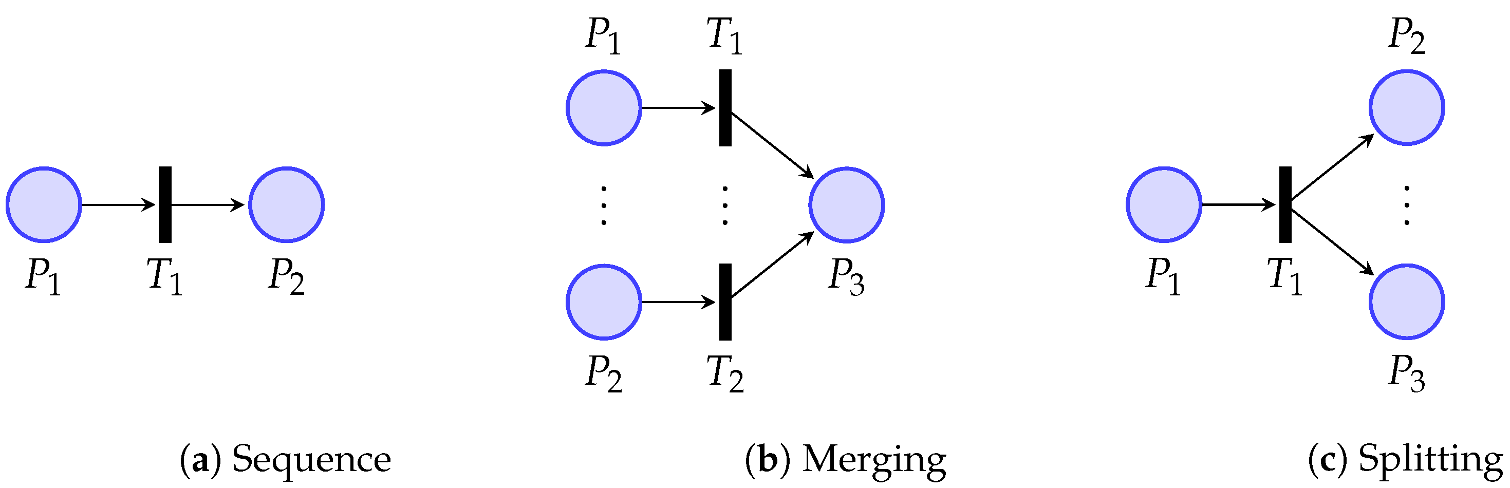
3.1. Introduction to Petri Nets

Before describing the automatic generation of the PN model of the JMPMSF, we formally introduce Petri Nets analogous to [17].
Definition 1 (Petri Net).
A Petri Net is a tuple P N = ( P , T , E , w , x 0 ) , where
  • P = { P 1 , . . . , P n } is a finite set of places, n N > 0 , graphically represented as circles,
  • T = { T 1 , . . . , T m } is a finite set of transitions, m N > 0 , graphically represented as bars,
  • E P × T T × P is a set of arcs from places to transitions and from transitions to places, graphically represented as arrows,
  • w : E N > 0 is an arc weight function, graphically represented as numbers labeling the arcs (if an arc has the weight 1 it is not labeled) and
  • x 0 N n is the initial marking of the Petri Net, from now on called initial state; the initial state of a place P i is graphically indicated by x i 0 dots (“tokens”) in the circle corresponding to P i .
The dynamics of a PN is driven by the firing of the transitions and captured by the evolution of the state vector x ( k ) N n at the time instants k N and is initialized with x ( 0 ) = x 0 . The firing of a transition T removes tokens according to the weights w ( P i , T ) of the arcs ( P i , T ) E from its input places P i P and adds token to its output places P o P according to the weights w ( T , P o ) of the arcs ( T , P o ) E . The number of times each transition fires at instant k is expressed with the firing count vector u ( k ) N m . We introduce the incidence matrix B = B + B which is composed of the two matrices B + N n × m and B N n × m that are defined as
B i , j + w ( T j , P i ) i f ( T j , P i ) E 0 e l s e B i , j w ( P i , T j ) i f ( P i , T j ) E 0 e l s e .
We can now compactly describe the Petri Net dynamics by
x ( k + 1 ) = x ( k ) + B u ( k ) , x ( 0 ) = x 0 .
As the places are not allowed to have a negative number of tokens, the Petri Net dynamics needs to be further restricted by only allowing transitions to fire if they do not generate negative tokens in any place. We say a transition T is enabled at a state x ( k ) if all of its input places P i connected through an arc ( P i , T ) E hold as least as many tokens as the arc weight w ( P i , T ) , i.e.,  x i w ( P i , T ) . Two transitions, T i and T j , might be concurrently enabled at state x ( k ) , but if they both fire simultaneously they would consume the same token resulting in a negative entry in the state vector x ( k + 1 ) . This situation is called conflict between the transitions T i and T j [39]. To prevent negative tokens in this case, a non-negativity condition on the basis of the firing count vector u ( k ) is introduced. With the matrix B and the state vector x ( k ) all allowed firing count vectors u ( k ) must satisfy the non-negativity constraint
0 x ( k ) B u ( k ) .

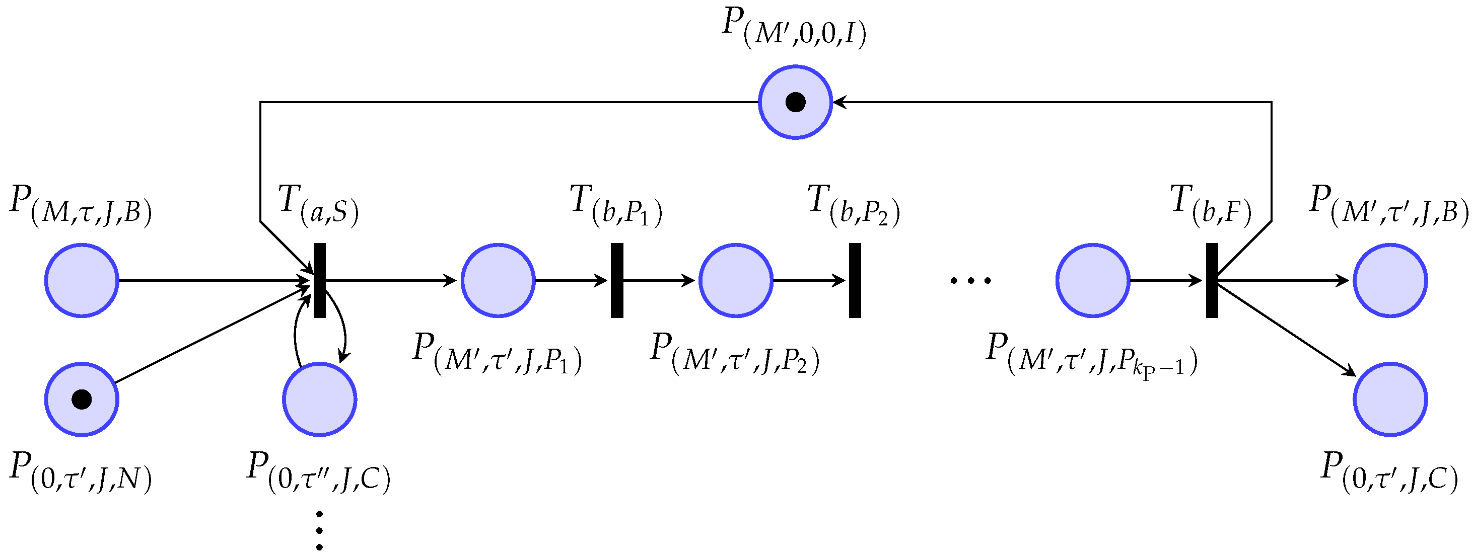
3.2. Modified Petri Net Dynamics

So far, we only introduced common notions for Petri Nets that can be found in literature, for example, in [39,40]. However, in order to describe the scheduling problem introduced in Section 2, we will slightly adapt the role of the transitions as proposed in our previous work [17]. In most literature on Petri Nets, the firing of transitions is initiated by predefined rules, considered to be stochastic, or the dynamics is even seen as the set of all possible sequences in which the transitions can fire [39,41]. In contrast to that, we will use a subset T C T of the transitions as controlled inputs to actively influence the dynamics of the Petri Net, which we will call controlled part of the PN, and another subset T I T of the transitions is defined to fire as soon as they are enabled, which we will call independent part of the PN.
As discussed by Giua and Seatzu [42], the PN dynamics (2) is a special case of the dynamics of a linear discrete time system x ( k + 1 ) = A x ( k ) + B u ( k ) with A = I , where I is the identity matrix of appropriate dimension. We will now exploit the possibility to change the matrix A such that it holds the influence of the so-called independent transitions in the set T I . The matrix B then merely considers the actively controlled transitions in the set T C and the control decisions are captured in the firing count vector u. Whether it is possible to represent the firing of a transition “as soon as it is enabled” and without violating the constraint (3) by means of a matrix multiplication A x of the PN’s state x with a matrix A, depends on its interconnection with the rest of the PN. Therefore, we introduce two restrictions on the independent transitions. A transition T can only be considered to be independent if
(I1)
it only has one input place P i ,
(I2)
its only input place P i has no second output transition,
(I3)
the weight of the arc ( P i , T ) connecting the place P i to its output transition T must be w ( P i , T ) = 1 .
With those restrictions, only the basic Petri Net elements depicted in Figure 1, i.e., sequence, merging, and splitting, can be assigned to the independent part of the Petri Net, i.e., to the set T I . On the other hand, conflict and synchronization depicted in Figure 2 must be controlled actively and the corresponding transitions always belong to the set  T C . This obviously also holds for the combination of synchronization and conflict in a so called non free-choice conflict [41].
With the distinction between independent transitions and controlled transitions, the Petri Net dynamics is described as
x ( k + 1 ) = A x ( k ) + B u ( k ) , x ( 0 ) = x 0 .
As the places must not hold a negative number of tokens, i.e., constraint (3) must still be satisfied, and as there always has to be an integer number of tokens, for the newly introduced dynamics matrix must hold A N n × n . The dynamics (4) together with the non-negativity constraint (3) is called state space description or state space form of the PN.
If the output transition T i of the place P i is handled as an independent transition, the i-th column of the matrix A is changed, starting from an identity matrix I for a completely controlled PN. The input arc ( P i , T i ) of transition T i sets the diagonal entry to zero, i.e.,  A i , i = 0 , and the output arcs ( T i , P o ) of the transition T i introduce the weight w ( T i , P o ) in the entry A o , i = w ( T i , P o ) . If a place has no independent output transition, a one in the corresponding diagonal entry in A keeps its number of tokens constant when no controlled transition fires.
Example 1.
The matrices corresponding the the elementary PN structures in Figure 1 are
A ( a ) = 0 0 1 1 , A ( b ) = 0 0 0 0 0 0 1 1 1 and A ( c ) = 0 0 0 1 1 0 1 0 1 .
The firing of the independent transitions at the state x ( k ) removes all tokens from the input places through the zero in the corresponding diagonal entry of the matrix A. In the state x ( k + 1 ) , tokens are produced in the output places of the independent transitions through the non-zero off-diagonal elements in A.
Note that the criteria (I1)–(I3) are necessary so that a transition can be assigned to the set T I . If one of them is not fulfilled for a specific transition, it must be assigned to the set T C . However, it is still possible to assign transitions to T C if they fulfill the three criteria (I1)–(I3). For example, it is possible to set the transition T 2 in Figure 1b as controlled transition and assign it to T C . In this case, the dynamics of the Petri Net in Figure 1b is
x ( k + 1 ) = 0 0 0 0 1 0 1 0 1 x ( k ) + 0 1 1 u ( k ) .
We will exploit the independent transitions to have a production process running autonomously while the scheduling decisions are handled by means of controlled transitions. How the problem formulation in Section 2 can be automatically transformed into a Petri Net will be discussed in the next Section.

3.3. Generation of the Discrete Time Petri Net Model

Form the description of the JMPMSF in Section 2, we will automatically generate a Petri Net model with the algorithms presented in our previous work [17]. The generated PN model will provide all possible manufacturing decisions in the form of controlled transitions in the set T C . Their implications are captured in the matrix B of the algebraic description (4) and the decisions are taken by means of the firing count vector u. The automatic production process is represented through the independent transitions in the set T I and handled in the matrix A of the algebraic representation (4), as presented in Section 3.2.
The state of the Petri Net x represents the current status of the manufacturing system. In order to preserve the production related meaning of the elements of the PN components, we introduce distinct identifiers as labels for the places and transitions. By introducing corresponding vectors x ID and u ID , the state x and the input vector u are intuitively understandable and can be related to the elements in the production system. The identifiers hold information on the machine, the task  and the job to which the places and transitions refer. Additionally, we introduce a classifying character σ Σ = { S , F , P , B , I , N , C } to indicate the meaning of the places and transitions in the production process. The classifier S relates to “start”, F relates to “finish”, B to “buffer”, I to “idle”, N to “necessary”, and C to “completed”. This set of classifiers was specifically selected for the given production problem together with the desired model of it and the algorithms that translate between them, which will be presented in the sequel. This set of classifiers is certainly not the only possible one to implement a similar model generation. If further characteristics of the production problem are investigated or other restrictions are present, the set of classifiers can be changed and further Petri Net structures can be introduced.
The identifier of a place P has the form ( M , τ , J , σ ) , as a place can relate to one machine M M , one task τ T , one job J J and has the production related meaning that corresponds to its classifier σ Σ . With this notation it becomes obvious to which machine, which task  and which job a place P ( M , τ , J , σ ) relates and how its marking can be interpreted. If a place has no specific machine, task  or job it relates to, its identifier has a zero at the respective position. For example the marking of the place P ( M , 0 , 0 , I ) indicates whether the machine M is idle, which is independent of any specific task or job.
A transition connects at least two places and its production related role can be related to the places connected to it. Its identifier has the form ( M , M , τ , τ , J , σ ) , which indicates that the transition T ( M , M , τ , τ , J , σ ) connects places of the form P ( M , τ , J , σ ) , and P ( M , τ , J , σ ) . The identifiers of transitions only refer to one job J, since we assume dependencies between different jobs to arise only through the fact that they are produced in the same manufacturing system, as discussed in Section 2 and formulated in Restriction (R2). As a consequence, all places connected to the same transition either relate to the same job or they do not relate to any job at all.
Analogous to the algorithms presented in our previous work [17], the PN model of the manufacturing system is created with the Algorithms 1 and 2. The generated model is a discrete time description of the manufacturing system and the production processes are represented by chains of places P ( M , τ , J , P 1 ) , P ( M , τ , J , P 2 ) , , P ( M , τ , J , P k P ( M , τ ) ) . The number of production steps
k P ( M , τ ) = t P ( M , τ ) t s
for the execution of the task τ on the machine M is calculated with respect to the sampling time t s , which is also called sampling period. It is rounded to the next larger integer which means that for a large sampling time t s the resulting production time t P ¯ = k P t s might be larger than the true production time t P , i.e.,  t P ¯ t P .
Algorithm 1: Create Places [17].
Applsci 11 08145 i001
Algorithm 1 generates the set of places P for the Petri Net. First, in lines 1–3, the idle places  P ( M , 0 , 0 , I ) , which indicate whether a machine is working or not, are created for all machines M M . As it is assumed that all machines are idle at initialization, the idle places are marked with one token. This token is consumed by every transition starting the execution of a task on the respective machine and returned once the production is finished. Due to this mechanism it is guaranteed that every machine only executes one task at a time and therefore respects Restriction (R6).
In lines 4–14, the places for the statuses of the jobs J J are created. Every job J has a starting place P ( 0 , 0 , J , S ) , initialized in line 5 with one token, indicating that the production of the respective job has not yet been started. Once the production of a job starts, its token is moved according to the production process. Despite the token is not labeled and it can not be said that it stays the “same” token, the machine at which the job is being processed or was processed last can be deduced from the identifiers and the markings of the production and buffer places related to it. Those places are created in line 10. For every machine M with τ T M , the production places P ( M , τ , J , P i ) , i = 1 k P ( M , τ ) are created. They indicate at which machine M the task τ of job J is executed and how far its execution already proceeded. At the end of line 10, the buffer places  P ( M , τ , J , B ) are created. If a buffer place P ( M , τ , J , B ) is marked, this shows that the task τ of the job J was processed on machine M at last and that the semi-finished product of the job J is currently in the output buffer of machine M. By generating the production and buffer places for all possible machines that can execute each task, the selection of the machine that will eventually execute it is not predefined a priori and can be chosen during runtime. This structure enables the Flexibility (F1). In line 7, necessity places  P ( 0 , τ , J , N ) and completion places P ( 0 , τ , J , C ) are created for all tasks τ T J , which indicate the production progress of the job J. Besides that, the completion places are used to ensure that the precedence relations between the tasks are met and Restriction (R1) is respected. As it is assumed that no task in any job is already completed at initialization, the completion places are initialized unmarked whereas the necessity places hold one token indicating that the respective task needs to be executed once.
Algorithm 2: Create Transitions and Arcs [17].
Applsci 11 08145 i002
In Algorithm 2, the transitions and arcs that allow the possible evolutions of the system and implement the required constraints are generated. At first, in lines 5 and 6, the starting transitions T ( 0 , M , 0 , τ , J , S ) to start the jobs are created for every possible initial task of the jobs.
The other starting transitions T ( M , M , τ , τ , J , S ) allowing to start all further tasks in an arbitrary order only restricted by the precedence between the tasks, i.e., Restriction (R1), are generated in lines 15–18. Every starting transition is a synchronization of an idle place, a necessity place and a starting or buffer place as illustrated in Figure 3. Its three input places need to be marked before a starting transition is enabled and allowed to fire, which is why it has to be implemented as a controlled transitions. This is not a restriction, however, as actively choosing the sequence in which the different tasks of the different jobs are started on the available machines by means of deciding which starting transitions fire at a given time, exactly implements the desired Flexibilities (F3) and (F4). The starting of a task reserves the machine M that is used for its execution by consuming the token from the idle place P ( M , 0 , 0 , I ) . This guarantees that every machine is only used once at a time as required by Restriction (R6). By consuming the token from the necessity place P ( 0 , τ , J , N ) , it is indicated that the task τ will not be necessary any longer. The consumption of the token from the starting place P ( 0 , 0 , J , S ) or the buffer place P ( M , τ , J , B ) reserves the semi-finished product of the job J and guarantees that only one task of every job is executed at a time, as required by Restriction (R7). Each starting transition that starts the execution of a task τ consumes the token from all completion places P ( 0 , τ , J , C ) of the tasks τ T τ that need to be finished before the task τ can be started. Thereby it is guaranteed the task τ can only be started once its precedence constraints according to Restriction (R1) are fulfilled. The tokens are immediately returned to the completion places such that their production status is preserved. Starting transitions create a token in the first production place P ( M , τ , J , P 1 ) , indicating that the production starts.
The production transitions T ( M , M , τ , τ , J , P q ) , which are created in the lines 8 and 9, implement the production process as a sequence of production steps, similar to Figure 1a, as illustrated in Figure 3. They move tokens from one production place P ( M , τ , J , P q ) , q [ 1 , k P ( M , τ ) 1 ] to the next production place P ( M , τ , J , P q + 1 ) and are implemented as independent transitions.
The finishing transitions T ( M , M , τ , τ , J , F ) are created in lines 10 and 11 and have the form of a splitting similar to Figure 1c. They are considered to be independent as well. They consume the token from the last production place and return a token to the idle place P ( M , 0 , 0 , I ) of the machine M that finishes the production and store the semi-finished product in its output buffer P ( M , τ , J , B ) . Finally, they set the task τ completed by creating a token in the completion place P ( 0 , τ , J , C ) .
The state space description of the Petri Net in the form of the Equations (3) and (4) is created as introduced in Section 3.2. First, the initial state x 0 is initialized by assigning the initial markings of all places to it. The effects of the production and finishing transitions are represented in the matrix A. Starting from an identity matrix I, for every production transition T ( M , M , τ , τ , J , P q ) the diagonal entry corresponding to its input place P ( M , τ , J , P q ) is set to zero and a one is introduced in the same column in the line corresponding to its output place P ( M , τ , J , P q + 1 ) . The result is similar to matrix A ( a ) in Example 1.
For every finishing transition T ( M , M , τ , τ , J , F ) , the diagonal entry corresponding to its input place P ( M , τ , J , P k P ( M , τ ) ) is set to zero and ones are introduced in the same column in the lines corresponding to its output places P ( M , τ , J , B ) , P ( M , 0 , 0 , I ) , and P ( 0 , τ , J , C ) . The result is similar to matrix A ( c ) in Example 1.
For every starting transition T ( M , M , τ , τ , J , S ) , a column is added to the matrix B through the matrices B + and B as defined in Equation (1). The new columns in B + and B are initialized with zeros. In B a one is introduced in the lines corresponding to the input places P ( 0 , τ , J , N ) , P ( M , 0 , 0 , I ) , and P ( M , τ , J , B ) . The precedence relations among different tasks, which are considered through arcs from the completion places of other tasks τ , lead to further ones in the lines corresponding to possibly multiple places of the form P ( 0 , τ , J , C ) . In B + a one is introduced in the line corresponding to the first production place P ( M , τ , J , P 1 ) and further ones are introduced in the lines corresponding to the completion places P ( 0 , τ , J , C ) of the precedence relation, in order to keep their marking constant. Note that directly creating the matrix B and omitting the matrices B + and B would make the completion places obsolete and cancel out their effect. Additionally, the matrix B is required to formulate the non-negativity constraint (3). The input vector u has one entry for every starting transition.
The result of the Algorithms 1 and 2 is the Petri Net P N = ( P , T , E , w , x 0 ) and its state space description given by the matrices A , B + , B and the initial state x 0 . The state space description will be used for the scheduling scheme described in Section 4. As it was created by specific Algorithms it has some properties that will be exploited to prove important properties of the scheduling scheme. Those properties are discussed in the next section.

3.4. Analysis and Discussion of the Discrete Time Petri Net Model

Before using the Petri Net model generated in Section 3.3 for the scheduling of the JMPMSF in Section 4, we will analyze its state space description (4) together with the non-negativity constraint (3). Some specific properties that will be exploited to prove important properties of the proposed scheduling scheme in Section 4 are given in the following lemma from our previous work [18].
Lemma 1 (Properties of the automatically generated Petri Net).
For the Petri Net P N = ( P , T , E , w , x 0 ) generated with the Algorithms 1 and 2, the following properties hold:
(P1)
A steady state is a pair of state and input ( x s , u s ) with x s = A x s + B u s . As there is no steady state ( x s , u s ) with u s 0 , u s N m , we denote x s the steady state and omit the input u.
The fact that there is no steady state with u s 0 means that the Petri Net P N has no T-invariant ([39] Definition 11.4).
(P2)
The following statements are equivalent:
In the state x s no production is taking place, i.e., no production place P ( , P ) is marked ⇔ x s is a steady state.
(P3)
The initial state x 0 generated in Algorithm 1 is a steady state and x 0 N n .
(P4)
All parts x ¯ , x ^ N n of a steady state x s are themselves steady states, i.e.,
x s = x ¯ + x ^ = A x s x ¯ = A x ¯ , x ^ = A x ^ .
(P5)
The precondition of every firing, which needs to be satisfied according to the non-negativity condition (3) in order to start a production process, forms a steady state for all inputs u, i.e.,  B u = A B u u N m .
(P6)
A task which has been completed stays completed, i.e., once the completion places P ( , C ) are marked they stay marked.
(P7)
If x ( 0 ) N n then x ( k ) = A k x ( 0 ) N n for all k 0 and condition (3) is satisfied for x ( k ) with u ( k ) = 0 for all k 0 .
(P8)
Every state x eventually enters a steady state x s = A n x ⇔ there is a k ¯ < n for which A k ¯ = A ( k ¯ + 1 ) = A n .
(P9)
If an operation O = ( τ , J ) , i.e., a specific task τ of a job J, can be started at a steady state x s , 1 , it can also be started in all steady states x s , 2 reachable from x s , 1 through a legal firing sequence respecting (3), or it was already completed in x s , 2 .
A proof of the Lemma 1 can be found in Appendix A.
The Properties (P1)–(P6) define important features of steady states, that are not only important for theoretical analysis, but also required for a reasonable representation of a production system. If, in contrast to Property (P1), an action is necessary to keep the production system at rest, it tends to be unstable. If, in contrast to Property (P2), a production is going on while the system is at rest, either the model is flawed or the production does not yield any products, which would not be favorable. Initializing the system at rest as stated in Property (P3) is a common way of modeling. If Property (P4) was not fulfilled, there would be a steady state only due to two or more ongoing processes that cancel each other out. This can be reasonable for some models, for example, if the states describe inventory levels. In our case, however, as the individual products are tracked, this would imply that one process is progressing on a product while another one is reversing its effect, which is not desired. The absence of property (P5) would allow the start of a new production process to be only temporarily possible and after some time it would not be possible any more without any external causes. This might be caused by decaying products or tools, which are not considered in the presented setup. Property (P6) describes a production process without disintegrating products. The created PN does not violate the non-negativity constraint (3) by the independent evolution represented through the matrix A as Property (P7) states. This means that the model by itself does not lead to any states which do not have a reasonable real-world representation. In the described production system no endless production processes can be started, which is expressed through Property (P8), and Property (P9) shows that there are no restrictions in the sequence flexibility (F3) of the described JMPMSF, except the ones explicitly modeled through Restriction (R1).
The discrete time model introduced in Section 3.3 describes the evolution of the production process with respect to the sampling time t s . A smaller sampling time t s will lead to an increased state dimension, which results from Equation (5) and the creation of the production places in line 10 of Algorithm 1. On the other hand, a larger sampling time might lead to a more significant over approximation of the true production time t P by the discrete time model through the rounding in Equation (5). As a consequence, the sampling time t s should be chosen in accordance with the dynamics of the represented processes. If the manufacturing system has processes with vastly different time scales, it might be hard to find a good compromise. However, despite the increasing state dimension, the number of input variables, which has an even greater influence on the runtime of the optimization problem presented in Section 4, is independent of the sampling time. This alleviates the drawbacks of having a small sampling time and a large state dimension.
In the creation of the discrete time Petri Net model, several structures and mechanisms are created to represent the characteristics of the job shop with multipurpose machines and sequence flexibility. In the sequel, we will briefly highlight the most significant ones and discuss simplifications of the PN model for special cases of the JMPMSF as for example for the ordinary job shop problem.
The possibility to execute the same task on different machines, i.e., Flexibility (F1), is introduced through the different production places and buffer places for the same task introduced in the line 10 of Algorithm 1. For an ordinary job shop, the if-statement in line 9 is only true for a single machine leading to a single chain of production places and a single buffer place for every task of every job.
The assumption of having multipurpose machines in the JMPMSF, i.e., flexibility (F2), is considered in the for-loop in line 8 of Algorithm 1 together with the if-statement in line 9, which allows to restrict the possibilities of the machines. For single-purpose machines, those conditions represent the search for the single machine that is able to execute the currently investigated task and could be implemented more efficiently.
The sequence flexibility in the JMPMSF, i.e., Flexibility (F3), is respected through the multitude of starting transitions that are created in the for-loop which starts in line 12 of Algorithm 2. They allow to change the sequence in which the tasks τ T J in a job J are executed. If no precedence relation between the tasks τ and τ is present, both transitions T ( M , M , τ , τ , J , S ) , starting τ after τ , and  T ( M , M , τ , τ , J , S ) , starting τ after τ , are present in the PN. It is guaranteed that only one of them can fire since each of them requires a token at the buffer place after the execution of the respective other task. Without sequence flexibility, the if-statement in line 13 of Algorithm 2 would only be true for the single task τ that follows after the task τ , leading to a single starting transition of τ and recovering the given production sequence. Furthermore, the necessity places and completion places created in line 7 of Algorithm 1 would be obsolete in this special case.
Remark 1.
The presented mechanism of creating a Petri Net model for a scheduling problem is not unique. With similar algorithms, further mechanisms and properties of a manufacturing system can be represented, as, for example, a limited buffer at every machine, production capacities of the machines larger than one, or maintenance tasks that are represented by transitions that are not related to any job.
Remark 2.
The automatically created Petri Net and the resulting mixed integer programming model is not the smallest one that would be possible for the given JMPMSF. For example, the size of the state vector could be reduced by summarizing all the buffer places P ( M , τ i , J , B ) for the different tasks τ i T J of the same job J that can be executed at the same machine M into one buffer place P ( M , 0 , J , B ) . By that, however, the information which task in job J was executed last is removed from the state of the PN.

4. Model Predictive Control

On the basis of the state space description of the automatically generated Petri Net, we will now develop two similar scheduling schemes for the job shop with multipurpose machines and sequence flexibility (JMPMSF) based on Model Predictive Control (MPC). One of them was first described and analyzed in our previous work [18], and the other one is a more efficient adaption thereof. Although they are specifically designed for JMPMSFs as defined in Section 2, they are exemplary for arbitrary scheduling problems formulated as a PN of the form introduced in Section 3.2.
Using systems and control theory to analyze and influence PNs is not uncommon in the literature [41,42], and also MPC techniques are used [43,44,45]. In the context of MPC for PNs, usually either continuous or hybrid PNs are considered from the start, or fluidification of the Petri Net is used, meaning that the integer constraint is relaxed and the tokens are considered to be a fluid. Instead of a state x N n and a firing count vector u N m , a state x ˜ R 0 n and a flow vector u ˜ R 0 m are considered. This relaxation is used to avoid a high dimensional state space and simplify the problem [43,45]. It is known that this adaptation changes the properties of the PN and that it is mostly suited for models with a large number of tokens [46,47]. In our particular case, it violates the notion of the production problem defined in Section 2. In order to illustrate this, let us only consider a starting transition that fires by a non-integer amount smaller than one, e.g.,  u ˜ ( 0 ) ( 0 , 1 ) at instant k = 0 . This would mean that a task is only partially started and therefore also only partially executed through the independent part of the PN dynamics (4) with u ˜ ( k ) = 0 for k > 0 . The result is a partially completed task. Although it is not completely equivalent, this is comparable to the violation of Restriction (R4), i.e., that a task must not be interrupted, as an interruption would also lead to a partially completed task. If there is a reason why it is not allowed to interrupt a task the same reason usually prohibits to only start it partially.
An MPC formulation for a timed discrete PN was presented by Lefebvre [48,49]. It is tailored to a setup in which a PN needs to be transferred from an initial marking to a desired final marking in minimum time while avoiding critical markings in which uncontrollable transitions could fire. Due to this specific setup, it is not applicable to the our case and especially not to the more general type of scheduling objectives described in Section 2.2.
In the context of discrete manufacturing, MPC was applied for dynamic capacity adjustment of a production system with reconfigurable machine tools and job shop characteristics by Zhang et al. [50]. They consider a continuous optimization problem, which relaxes the integer constraint in the sense of fluidification of the problem. The question how the underlying integer assignment problem can be solved is left as an outlook. An MPC approach for the scheduling of reentrant manufacturing lines motivated by semiconductor manufacturing was considered by Vargas-Villamil and Rivera [51], who optimize a the long-term behavior of a reentrant production system modeled as a discrete-time flow model with respect to a multi-objective cost function by means of linear programming. The result of the MPC is fed to a subordinate controller which coordinates the short-term decisions and applies the integer valued control input to the plant. Cataldo et al. [52] use MPC for the scheduling in a machine environment with parallel identical machines that are fed through transportation lines of different lengths. The goal is to maximize the production output while limiting the energy consumption. The resulting optimization problem is a MIP assigning speeds to the machines and binary inputs to the transportation system. For general job shop problems no alternative MPC approach was found in the literature.
In contrast to problems in scheduling and discrete manufacturing where MPC is rarely used [52], it has a variety of applications in supply chain management and especially in process industry, where continuous models naturally arise [53,54,55,56]. Due to the large body of knowledge on various properties and different implementations of MPC schemes, it became a well-established control method [57].
In the sequel, we start by formulating the first MPC problem according to [18], before we show that the problem is feasible in Section 4.2 and determine a criterion to guarantee the completion of a single operation in the production problem in Section 4.3. The insights form this discussions motivate the formulation of the second MPC formulation in Section 4.4. The guarantees for the completion of the production problem for both MPC formulations are given in Section 4.5.

4.1. Formulation of the MPC Problem

As discussed in Section 2.2, the goal of the proposed production scheduling scheme is to optimize the profitability of the production system. This is done by assigning the different tasks to the most efficient machines and by choosing the production sequence which yields the most reward possible. In order to quantify the profitability of the production system represented as a PN, we introduce a cost function c : N n × N m R , which is called stage cost, that assigns to every pair ( x , u ) of state and input a cost value c ( x , u ) . It quantifies how much cost the current status of the production system represented through the state x and the decisions taken through the input u cause. In general, the cost may depend arbitrarily on x and u and can also contain couplings between them. As the state of the system changes over time and at every time step new decisions are taken, the cost c ( x ( k ) , u ( k ) ) only represents the cost in the current time interval of length t s . In order to achieve a good performance with respect to a given cost function c, the system needs to be influenced in a way such that the resulting cost summed up over time is minimal. In the sense of MPC, we formulate this goal as a finite horizon optimal control problem over the prediction horizon N, which is repeatedly solved in a rolling horizon fashion [14]. It is initialized at each time instant k with the most accurate knowledge about the system, which is the state x ( k ) that we assume to be known or measured. This assumption is justified by the concept of the digital twin introduced in Section 1. The optimization problem to determine the MPC control law at time instant k is formulated as
minimize u ( · | k ) k ¯ = 0 N 1 c x k ¯ | k , u k ¯ | k
subsect to x k ¯ + 1 | k = A x k ¯ | k + B u k ¯ | k
0 x k ¯ | k B u k ¯ | k
u k ¯ | k N m
x 0 | k = x k .
During the prediction, the PN dynamics (4) and the non-negativity of the states (3) need to be respected in the constraints (6b) and (6c). The planned input vectors u ( k ¯ | k ) are only allowed to have non-negative integer values (6d), whereby also the predicted states x ( k ¯ | k ) remain vectors of of non-negative integers and the tokens in the PN are moved in the intended direction. The optimization variables in the MPC problem are the inputs u ( k ¯ | k ) of the planned input trajectory u ( · | k ) = x ( 0 | k ) , , u ( N 1 | k ) . They allow to choose a new firing count vector u ( k ¯ | k ) at every future time instant k + k ¯ and represent potential decisions taken for the production process. The minimizer of (6a) in the MPC problem is the optimal input trajectory u * ( · | k ) . The resulting optimal predicted state trajectory, which results from applying the inputs u * ( · | k ) starting from the initial state x ( k ) , is denoted x * ( · | k ) . The sum of the predicted cost is only minimized over a finite prediction horizon N N > 0 in Equation (6a). This is not only the common case in MPC, but also reasonable under the assumption that the production system changes over time due to unknown or uncertain external influences. Due to such disturbances, the predictions for the distant future are unlikely to be accurate. From the optimal input trajectory u * ( · | k ) , only the first input u * ( 0 | k ) is applied to the system, before the optimization is repeated with the newly measured state x ( k + 1 ) at the next time instant. The resulting nominal closed loop dynamics can be expressed as
x ( k + 1 ) = A x ( k ) + B u * ( 0 | k ) = x ( 1 | k ) , x ( 0 ) = x 0 ,
where a feedback mechanism is introduced through the repeated solution of the optimization problem (6). This inherent feedback mechanism is one of the key features of the presented approach compared with scheduling techniques from literature [22,23]. It is necessary as, due to external influences and non-modeled effects, the state x ( 1 | k ) , which was predicted for time k + 1 starting from x ( k ) and applying u * ( 0 | k ) , might be different from the true state x ( k + 1 ) . Therefore, for the real closed loop it might be x ( k + 1 ) x ( 1 | k ) .
In order to provide a proof that the proposed MPC scheme leads to a desirable solution of the scheduling problem defined in Section 2, we first need to show important properties. Repeatedly applying the optimal input determined through a finite horizon optimal control problem such as (6) does not naturally lead to an optimal closed loop performance [58], which in our case is the completion of all jobs in the production problem in the best possible way. In fact, quite the opposite can be the case, and the MPC might not even start a single task if the MPC problem (6) is not formulated carefully and does not fulfill some required conditions. In this respect, the MPC problem is analyzed in the following sections and guarantees are provided that the desired properties, i.e., always having a feasible solution and leading to a state in which the production problem is completed, are fulfilled if some specific conditions are satisfied. We first show that there always exists a solution to the optimization problem (6) in the following section, before we provide conditions on the cost function c ( x , u ) and the prediction horizon N which guarantee that applying the MPC to the manufacturing system will lead to the completion of every task in every job and therefore to the completion of the scheduling problem.

4.2. Feasibility of the MPC Problem

As a first important property of the MPC problem formulated in Section 4.1, it needs to be guaranteed that the optimization problem (6) always has a feasible solution when it is applied in closed loop (7), which is called recursive feasibility in the context of MPC [14]. Proving recursive feasibility of an MPC problem requires prior assumptions. In our case, the standing assumption is that the PN was generated with the Algorithms 1 and 2 for a manufacturing system as described in Section 2. We first show that under this assumption the MPC optimization problem (6) is feasible for every possible state of the PN, before specifically analyzing the closed loop system (7).
Lemma 2 (Feasibility).
For every Petri Net P N = ( P , T , E , w , x 0 ) generated with the Algorithms 1 and 2 represented in its state space form (3), (4), the MPC optimization problem (6) is feasible for all x ( k ) N n .
Proof of Lemma 2.
The input trajectory u ( · | k ) = ( 0 , , 0 ) satisfies (6d), and for all x ( k ) N n it satisfies constraint (6c) due to Property (P7). Constraint (6b) is satisfied with x ( k ¯ + 1 | k ) according to the open loop system dynamics (4). Therefore u ( · | k ) = ( 0 , , 0 ) is a feasible candidate solution of the MPC Problem (6) for every x ( k ) N n . For the PN generated with the Algorithms 1 and 2 it particularly holds that x 0 N n due to Property (P3).    □
Lemma 3 (Recursive feasibility).
For every Petri Net P N = ( P , T , E , w , x 0 ) generated with the Algorithms 1 and 2 represented in its state space form (3), (4), the MPC optimization problem (6) is feasible with x ( k ) = x 0 , the nominal closed loop system (7) with u * ( 0 | k ) from problem (6) satisfies the condition (3), and Problem (6) is feasible for all k N .
Proof of Lemma 3.
From Lemma 2 and as x 0 N n due to Property (P3) follows that the input trajectory u ( · | k ) = ( 0 , , 0 ) is a feasible candidate solution at x ( k ) = x 0 .
That the nominal closed loop system (7) with u * ( 0 | k ) from problem (6) satisfies the condition (3) follows directly from the fact that x ( k ) = x ( 0 | k ) holds in the nominal case and since u * ( 0 | k ) satisfies (6c).
For every feasible input trajectory u ( · | k ) at time instant k, the input trajectory u ( · | k + 1 ) = u ( 1 | k ) , , u ( N 1 | k ) , 0 is a feasible input trajectory to Problem (6) at time k + 1 with the initial state x ( 0 | k + 1 ) = x ( k + 1 ) = x ( 1 | k ) from the nominal closed loop system (7). The feasibility of the inputs u ( 0 | k + 1 ) = u ( 1 | k ) , , u ( N 2 | k + 1 ) = u ( N 1 | k ) follows directly from the feasibility of u ( · | k ) at time instant k. The final predicted input u ( N 1 | k + 1 ) = 0 is also feasible due to the following reasons. First, it naturally satisfies constraint (6d). The predicted state x ( N 1 | k + 1 ) is a natural number, i.e.,  x ( N 1 | k + 1 ) N n , due to the feasibility of u ( N 2 | k + 1 ) = u ( N 1 | k ) and satisfies the constraint (6b) according to the open loop system dynamics (4). For x ( N 1 | k + 1 ) N n , constraint (6c) is satisfied with u ( N 1 | k + 1 ) = 0 due to Property (P7).    □
The input trajectory u ( · | k ) = ( 0 , , 0 ) used in the proof of Lemma 2 simply does not start any task in the scheduling problem. This is surely not desired but in the problem described in Section 2 there is no external driver prohibiting this solution. In the same sense, extending an existing feasible input trajectory u ( · | k ) by a new predicted input u ( N 1 | k + 1 ) = 0 in the candidate trajectory for the next time step used in the proof of Lemma 3 does not plan to start any new task in the last step of the prediction.
As explained in Section 2.2, there is a production related objective that requires taking some action due to its economic motivation. This objective needs to be formulated in the form of a cost function c ( x , u ) depending on the state x and the input u. In the sequel we will investigate properties of such a cost function, which we assume to be known and given, that allow to adjust the prediction horizon N such that the production problem controlled with the MPC is guaranteed to be completed. In this process we exploit the hierarchical nature of the production problem that is composed of jobs, which themselves are composed of tasks. We first provide a sufficient condition for the completion of a single operation, i.e., a single task of a single job. The arguments in the proof of the completion of an operation motivate the formulation of a more efficient MPC scheme. Finally, we provide a condition for the completion of a job and finally of the whole production problem for both MPC schemes.

4.3. Completion of an Operation

Our goal is to achieve optimal performance of the system in closed loop through applying MPC. For a flexible manufacturing system (FMS), the first and most important goal is to produce the requested products. In the formulation of the production problem in Section 2, this means the completion of all the tasks of all jobs. In the model generated in Section 3, this is represented as the convergence to a state in which all completion places are marked. In this section, we will first guarantee the completion of a single operation if some clearly specified condition are fulfilled.
A second goal in an FMS is to minimize production cost or to maximize profit. This can be conveniently formulated with a cost function. In the MPC, this cost function is directly use as objective function of the optimization problem (6a). As the cost function is only optimized over a limited prediction horizon N, the reward of performing actions in the manufacturing system needs to be perceived through evaluating the cost function during this limited time frame. This results in a condition on the cost function c ( x , u ) and subsequently in a condition on the prediction horizon N. In the sequel we will show how the prediction horizon N must be chosen based on the given manufacturing system as described in Section 2 and a given cost function c ( x , u ) in order to guarantee completion of a specific operation O = ( τ , J ) in the production problem with the MPC. To achieve this result, we first give a general condition that must hold such that the MPC completes any operation.
Lemma 4 (Starting an operation).
Given a Petri Net of a flexible manufacturing system in its state space form (3), (4) is generated with the Algorithms 1 and 2. If for a steady state x s all optimal input trajectories u * ( · | k ) for the MPC problem (6) initialized at x ( k ) = x s are such that u * ( 0 | k ) 0 , then at least one operation O = ( τ , J ) will be started at time instant k in closed loop (7), the operation O will eventually be completed, and it will remain completed.
Proof of Lemma 4.
In Algorithm 2, the only transitions that are added to the set of controlled transitions T C are starting transitions T ( , S ) . Therefore, every optimal first input u * ( 0 | k ) 0 fires at least one starting transition and thereby initiates the execution of at least one operation by marking at least one production place P ( , P 1 ) . The first input u * ( 0 | k ) is applied to the closed loop system controlled by the MPC (7) at time instant k. Therefore the production is not only started in the prediction, but also in closed loop. According to Property (P2), the resulting state is no steady state as a production place P ( , P 1 ) is marked. Due to Property (P8), eventually another steady state is reached. According to Property (P2), a steady state is only reached when no production place P ( , P ) is marked any more. As the only independent transitions T T I that do not mark another production place are finishing transitions T ( , F ) , this means that eventually a finishing transition fires. As every finishing transition T ( , F ) created in lines 10 and 11 of Algorithm 2 marks a completion place P ( , C ) , eventually a completion place is marked. Due to Property (P6), once completion places are marked they stay marked and hence the completed operations stay completed.    □
The condition in Lemma 4 can be exploited to guarantee the completion of a given production problem as long as it is finite and feasible, which we state in the following assumptions. As we generally allow the production problem to change, for example, through new jobs in the production problem, we assume that it is finite and feasible at the time when we investigate it. For a production problem that can always be extended, trying to argue that it will be completed a certain point in time is futile. Therefore, we will only analyze the properties of the production problems as it is at a certain point in time.
Assumption 1 (Finite production system).
The given production problem formulated as in Section 2 is finite, meaning that it has a finite number of possible tasks n τ < , a finite number of jobs n J < and a finite number of machines n M < at a given time.
We state the central assumption that the production problem is feasible, meaning that all operations can be executed by the given machine pool, on the level of the initial production problem formulated in Section 2 as well as on the level of the Petri Net and its state space description described in Section 3.
Assumption 2
(Feasibility of the production problem [18]). All jobs J J can be fulfilled by the given production system. This means that for every job J J and every task τ T J there exists at least one machine M M with τ T M .
In terms of the Petri Net, there exists at least one state x ^ in which every completion place P ( , C ) is marked and which is reachable from the initial state  x 0 .
In the state space, there exists at least one state x ^ with x ^ i = 1 for every i where x i ID = ( , C ) and which is reachable from from the initial state x 0 , i.e., there exists a legal input trajectory ( u ( 0 ) , , u ( k ^ 1 ) ) leading from x ( 0 ) = x 0 to x ^ = x ( k ^ ) = A k ^ x 0 + l = 0 k ^ 1 A l B u ( k ^ 1 l ) and where the non-negativity constraint (3) is respected for all x ( k ) , u ( k ) with k = 0 , , k ^ .
Lemma 5 (Completion of the production problem).
Given a Petri Net of a flexible manufacturing system in its state space form (3), (4) generated with the Algorithms 1 and 2 that fulfills the Assumptions 1 and 2. If there is only one steady state x F for which not all optimal input trajectories u * ( · | k ) for the MPC problem (6) are such that u * ( 0 | k ) 0 , then the production problem will be completed by the MPC and x F is the final state of production system.
Proof of Lemma 5.
The steady state x F is the only steady state for which the preconditions of Lemma 4 are not fulfilled. For all other steady states x s , all optimal input trajectories u * ( · | k ) for the MPC problem (6) are such that u * ( 0 | k ) 0 . Therefore, Lemma 4 states that in all steady states except x F at least one operation O is started. As the production problem is feasible due to Assumption 2, all operations can be executed and since it is finite due to Assumption 1, there is only a finite number of possible operations to be started, so eventually all operations had been started. Due to Property (P8) another steady state will be reached. As x F is the only steady state for which the preconditions of Lemma 4 are not fulfilled, it is the only steady state in which the system can remain.    □
The condition in Lemma 5 that there only exists a single final state x F is more restrictive than necessary. In general, also for a fixed production problem there is a set X F of final states, in which no further production is possible and all jobs are completed. The convergence to this set can be shown with similar arguments.
Having stated very general conditions when an MPC executes operations and ultimately completes the production problem, we will now formulate more specific conditions on the prediction horizon N and the cost function c ( x , u ) which guarantee the completion of an operation O = ( τ , J ) . As proposed in [18], we will use the cost function c ( x , u ) in the MPC problem (6) to determine a sufficiently long prediction horizon N O to guarantee the completion of the operation O for all prediction horizons N N O . In order to proof the finalization of every operation, we first define the sets X O , S and X O , C to classify the steady states in which an operation O can be started and the steady states in which it was just finished, respectively.
Definition 2
([18]). For every O = ( τ , J ) with τ T J , J J , the set X O , S is defined as the set of steady states in which the operation O can be directly started and which is reachable from the initial state of the production system x 0 through a legal input trajectory.
Definition 3
([18]). sFor every O = ( τ , J ) with τ T J , J J , the set X O , C is defined as the set of steady states right after the operation O was completed starting from a state x O , S X O , S without executing any further task.
Theorem 1
(Completion of an operation [18]). Given a Petri Net of a flexible manufacturing system in its state space form (3), (4) generated with the Algorithms 1 and 2 that fulfills the Assumptions 1 and 2. If for an operation O = ( τ , J ) and a cost function c ( x , u ) holds that for every state x O , S X O , S there exists a state x O , C X O , C reachable from x O , S with
c ( x O , S , 0 ) > c ( x O , C , 0 )
then there exists a shortest sufficient prediction horizon N O N > 0 with the property that for every N N O the operation O will eventually be executed when starting from any x 0 X O , S and applying the optimal solution to the MPC problem (6) in closed loop (7).
Proof of Theorem 1.
As shown in Lemma 4, an optimal input trajectory u * ( · | k ) with the first predicted input u * ( 0 | k ) 0 is required such that some operation is started. In order to prove that the investigated operation O is started, we need to show that the closed loop system always enters a state in which the optimal input trajectory has an input u * ( 0 | k ) U O , S as first planned input, where U O , S is the set of all input vectors u that start the execution of operation O.
Part I:
We only investigate the point in time when the operation O is started in this part of the proof. Therefore, we assume that the considered operation O = ( τ , J ) is the only operation that can be started and also the only one that needs to be executed in x O , S . For this case, we split all possible predicted trajectories into four categories and compare their resulting cost over the prediction horizon N. Without loss of generality, we consider all cases to lead towards the same state x O , C X O , C , for which condition (8) holds, except the fourth case where this exception it explicitly mentioned.
  • The operation O is not executed at all and thus the first predicted input is u ( 0 | k ) U O , S . As no other operation can be executed, the resulting cost over the prediction horizon N is
    c N , 0 = N c ( x O , S , 0 ) .
  • The operation O is planned to start immediately, i.e., at k ¯ = 0 , on some machine M M with τ T M leading to the steady state x O , C . In this case, the first predicted input is u ( 0 | k ) U O , S . As no other operation needs to be executed after finishing the execution of the operation O, the resulting cost over the prediction horizon N is
    c N , 1 = c P ( M , O ) + N k P ( M , τ ) c ( x O , C , 0 ) ,
    where c P ( M , O ) is the production cost of the operation O on machine M.
  • The operation O is planned to start at a later point in time, let us say at k ¯ = k ^ , on some machine M M with τ T M , but it is still completely executed and the steady x O , C is reached in the prediction. In this case, the input u ( k ^ | k ) U O , S , but the first predicted input is u ( 0 | k ) U O , S . The resulting cost over the prediction horizon N is
    c N , 2 = c P ( M , O ) + k ^ c ( x O , S , 0 ) + N k P ( M , τ ) k ^ c ( x O , C , 0 )
    as no other operation can be started in x O , S and thus the system stays in x O , S for k ^ time steps.
  • The operation O is planned to start at an even later point in time on some machine M M with τ T M , such that it is not completely executed any more but only the first k ˜ production steps, and no steady is reached at the end of the prediction. As no steady state is reached, the execution of O on M might or might not lead to x O , C after the prediction horizon. In this case, the input u ( N k ˜ | k ) U O , S , but the first predicted input is u ( 0 | k ) U O , S . The resulting cost over the prediction horizon N is
    c N , 3 = c P ˜ ( M , O ) + ( N k ˜ ) c ( x O , S , 0 )
    where c P ˜ ( M , O ) is the cost of the first part of the execution of O on M . No other operation can be started in x O , S and thus the system stays in x O , S for N k ˜ time steps.
As the MPC scheme (6) minimizes the cost over the prediction horizon N, the optimal first input u * ( 0 , k ) of the case with the lowest cost will be applied to the system. This means that the operation O will be executed in closed loop if c N , 0 > c N , 1 ,   c N , 2 > c N , 1 and c N , 3 > c N , 1 , which means that the immediate execution of the operation O yields most benefit over the prediction horizon N. As the existence of a lower bound N O for the prediction horizon needs to be proven, we can assume N N O > k P ( M , τ ) for all M with τ T M . With this assumption, also the effect of the production cost c P ( M , O ) and the number of production steps k P ( M , O ) will be negligible, as the following considerations show. First note that due to condition (8) and as k ^ > 0 it always holds that
c N , 2 > c N , 1 c P ( M , O ) + k ^ c ( x O , S , 0 ) s o m e t h i n g x x + N k P ( M , τ ) k ^ c ( x O , C , 0 ) > c P ( M , O ) s o m e t h i n g l o n g e r r r r r x x + N k P ( M , τ ) c ( x O , C , 0 ) k ^ c ( x O , S , 0 ) c ( x O , C , 0 ) > 0 .
For c N , 0 > c N , 1 to hold, it follows with Equations (9) and (10)
N c ( x O , S , 0 ) > c P ( M , O ) + ( N k P ( M , τ ) ) c ( x O , C , 0 ) N > c P ( M , O ) k P ( M , τ ) c ( x O , C , 0 ) c ( x O , S , 0 ) c ( x τ , C , 0 ) .
For c N , 3 > c N , 1 to hold, it follows with Equations (10) and (12)
c P ˜ ( M , O ) + ( N k ˜ ) c ( x O , S , 0 ) > c P ( M , O ) + N k P ( M , τ ) c ( x O , C , 0 ) N > c P ( M , O ) c P ˜ ( M , O ) + k ˜ c ( x O , S , 0 ) k P ( M , τ ) c ( x O , C , 0 ) c ( x O , S , 0 ) c ( x O , C , 0 ) .
As the right hand sides of (14) and (15) only depend on system parameters that are assumed to be known, these inequalities can always be fulfilled with a large enough value of N. In the cases where a final steady state is reached, all trajectories that lead to a steady state x C , 1 with higher cost as x O , C , i.e.,  c ( x C , 1 , 0 ) > c ( x O , C , 0 ) , clearly lead to higher cost over a large prediction horizon N and will not be the optimal input trajectory u * ( · | k ) . In the fourth case, choosing a trajectory that does not lead to x O , C only changes c P ˜ ( M , O ) . From Equation (15) it can be seen that an arbitrary, possibly even negative, production cost of the first production steps c P ˜ ( M , O ) can still be compensated by increasing N.
Part II:  
Suppose there is at least one other operation O that can be executed at x O , S , i.e.,  x O , S X O , S , then there are two possibilities:
  • O and O are executed at the same time,
  • O and O are not executed at the same time, either because there is no input vector u starting O and O and satisfying the non-negativity constraint (3), or because only executing one of them leads to a better solution of the MPC problem (6), i.e., an input trajectory u * ( · | k ) that leads to lower cost over the prediction horizon N.
In the case A, we know that the system will enter another steady state x C , 2 due to Property (P8). To proof the existence of the shortest sufficient prediction horizon, we have to assume that x C , 2 is reached during prediction, which can be achieved by increasing N. We neither have any information on the cost of the resulting steady state x C , 2 after the completion of both operations, nor do we have information on the number of production steps and the production cost of both operations at the same time. As for the considerations in the cases in Part I, in which only the operation O can be started, the effects of the number of production steps and the production cost can be compensated by increasing N. If the cost of the resulting steady state x C , 2 is smaller than the cost of the initial state x O , S , i.e.,  c ( x C , 2 , 0 ) < c ( x O , S , 0 ) , the same arguments as in Part I prove that leaving x O , S immediately in order to reach x C , 2 as soon as possible is the optimal choice and thus with u * ( 0 | k ) either O, or  O , or both are started. If O or both operations are started, the proof is completed. If another operation O is started with u * ( 0 | k ) U O , S , it is not directly guaranteed that O will be started. However, due to Properties (P8) and (P9), the closed loop system will then eventually enter another steady state x O , S , 2 X O , S . In this state, due to the precondition of Theorem 1, there is another steady state x O , C , 2 X O , C , for which all the arguments in this proof apply. As there are only finitely many operations due to Assumption 1, this recursion can only occur finitely often and eventually the system will enter a steady state x O , S , 3 X O , S in which due to the precondition of Theorem 1 a steady state x O , C , 3 X O , C exists and the operation O is executed. This happens at latest if O is the only operation left and the arguments in Part I hold. Note that instead of O also multiple operations at the same time can be considered in this paragraph on the case A.
In the case B, in which the operations O and O are executed sequentially, either O is executed first and, due to the same arguments as in Part I, will be executed immediately. Or operation O is executed first, which can only occur if the execution of O yields more benefit over the prediction horizon N as the execution of O. As argued in Part I, this can only be in combination with a steady state x O , C X O , C with c ( x O , C , 0 ) < c ( x O , S , 0 ) . Therefore, the arguments used in Part I prove that operation O is executed immediately through an input vector u * ( 0 | k ) U O , S . Due to the Properties (P8) and (P9), the closed loop system will then eventually enter another steady state x O , S , 2 X O , S for which due to the precondition of Theorem 1, there is a steady state x O , C , 2 X O , C satisfying condition (8), for which all the arguments in this proof apply. As argued in the case A, this recursion can only occur finitely often due to Assumption 1, which proves the ultimate completion of the operation O.    □
Theorem 1 shows that a cost decrease between starting states and completion states drives the production process. Through the arguments to prove Theorem 1, it can be seen that such a cost decrease combined with a long enough prediction horizon N incentivizes an immediate start of operations. Therefore, it implicitly leads to a minimization of the production time, or at least to a short production time under consideration of the given cost function. With Theorem 1, a rigorous condition is provided to examine whether a large enough prediction horizon can lead to the guaranteed completion of the investigated operation. The proof of Theorem 1 illustrates, however, that a cheap initial state combined with cheap production processes and expensive final states can lead to the situation in which the optimal predicted trajectory stays in the initial state for some time before the production process is planned to be initiated. As only the optimal first input u * ( 0 | k ) = 0 is applied, under those circumstances no production is started at all.

4.4. MPC Formulation with Terminal Cost

Theorem 1 is based on extending the prediction horizon N such that staying at a final steady state x O , C with low cost c ( x O , C , 0 ) for a long amount of time will incentivize the immediate start of an operation. due to Property (P8), this leads to the completion of the investigated operation. This insight can be used to formulate a more efficient MPC problem with terminal cost that has similar properties:
minimize u ( · | k ) k ¯ = 0 N 1 c x k ¯ | k , u k ¯ | k + V f x ( N | k )
subsect to x k ¯ + 1 | k = A x k ¯ | k + B u k ¯ | k
0 x k ¯ | k B u k ¯ | k
u k ¯ | k N m
x 0 | k = x k .
In this formulation, the terminal cost V f : N n R is introduced with respect to the previous formulation of the MPC problem (6). It can be used in order to capture the cost of resting in a final steady state for an extended amount of time. By assigning
V f x = k ¯ = 0 N + c ( A k ¯ x , 0 ) ,
the cost of assigning the input u ( k ¯ | k ) = 0 for k ¯ = N , , N + N + to the system is evaluated through V f x ( N | k ) . This strategy to enlarge the prediction horizon by finite amount N + over which the control input is kept constant is a well-known strategy in MPC literature [59]. It is known that capturing the cost over this extended period of time in a terminal cost can be used to prove stability of the closed loop system. due to Property (P8), for a sufficiently long extended prediction horizon N + the system converges to a steady state and stays there as long as the input u ( k ¯ | k ) = 0 is applied. With this insight, we can formulate the following corollary.
Corollary 1 (Completion of an operation with the MPC with terminal cost).
Given a Petri Net of a flexible manufacturing system in its state space form (3), (4) generated with the Algorithms 1 and 2 that fulfills the Assumptions 1 and 2. If for an operation O = ( τ , J ) and a cost function c ( x , u ) holds that for every state x O , S X O , S , there exists a state x O , C X O , C reachable from x O , S with
c ( x O , S , 0 ) > c ( x O , C , 0 )
then there exists a shortest sufficient extended prediction horizon N O + N > 0 with the property that for every N + N O + and every N N > 0 the operation O will eventually be executed when starting from any x 0 X O , S and applying the optimal solution to the MPC problem (16) with the terminal cost (17) in closed loop (7).
Proof of Corollary 1.
The proof is analogous to the proof of Theorem 1. First, note that staying in the final state x O , C is beneficial compared with staying in x O , S due to condition (18). due to Property (P8), this final state will be reached as soon an input u * ( 0 | k ) U O , S starting the operation O is applied. The terminal cost V f defined in Equation (17) is the cost of finishing all running production processes and then staying at the final steady state. With every prediction horizon N > 0 , the MPC selects the best possible inputs during the first N steps considering the autonomous continuation of the processes for further N + time steps after the prediction horizon.
In every prediction horizon N > 0 starting at a state x O , S X O , S , the possibility of immediately starting a process leading from x O , S to x O , C , i.e., applying an input u * ( 0 | k ) U O , S , is considered in the optimization. If the horizon N + N + , over which the cost is considered, is long enough, it follows from the same arguments as in the proof of Theorem 1 that applying the input u * ( 0 | k ) = 0 and not starting any operation can not be more beneficial than immediately starting some operation O . Due to condition (18), one possibility would be O = O . As there might be other beneficial inputs starting other operations O , the operation that is immediately started does not have to be the investigated operation O. As soon as N + N + is large enough, however, a condition as (18) also needs to hold for the operation O if it is optimal to start it through an input u * ( 0 | k ) U O , S . Therefore, as shown in the proof of Theorem 1, it is always better to start such an operation immediately compared with starting it later. Due to Properties (P8) and (P9) and finiteness of the production problem assumed in Assumption 1, it is guaranteed that at some point in time the closed loop (7) reaches a state in which applying u * ( 0 | k ) U O , S is the optimal solution of the MPC problem (16).    □

4.5. Completion of the Production Problem

In the previous section, we have proven the completion of an operation O when either the MPC (6) or the MPC with the terminal cost (16) and the terminal cost function (17) is applied in closed loop, which is formulated in Theorem 1 and Corollary 1. This is the basis to guarantee the completion of every job and therefore of the entire production problem.
Corollary 2
(Completion of a job [18]). Given a Petri Net of a flexible manufacturing system in its state space form (3), (4) generated with the Algorithms 1 and 2 that fulfills the Assumptions 1 and 2. If for every task τ T J of a job J there exists
(a)
a shortest sufficient prediction horizon N O for the operation O = ( τ , J ) , then there exists a shortest sufficient prediction horizon N J = max τ T J N O with the property that for every N N J the job J will eventually be completed when applying the MPC (6) in closed loop (7) from any initial state x 0 X J , S τ T J X O , S .
(b)
a shortest sufficient extended prediction horizon N O + for the operation O = ( τ , J ) , then there exists a shortest sufficient extended prediction horizon N J + = max τ T J N O + with the property that for every N N > 0 and every N + N J + the job J will eventually be completed when applying the MPC (16) with the terminal cost (17) in closed loop (7) from any initial state x 0 X J , S τ T J X O , S .
Corollary 3
(Completion of the production problem [18]). Given a Petri Net of a flexible manufacturing system in its state space form (3), (4) generated with the Algorithms 1 and 2 that fulfills the Assumptions 1 and 2. If for every job J J there exists
(a)
a shortest sufficient prediction horizon N J , then there exists a shortest sufficient prediction horizon N min = max J J N J with the property that for every N N min the given production problem will eventually be completed when applying the MPC (6) in closed loop (7) from any initial state x 0 X S J J X J , S .
(b)
a shortest sufficient extended prediction horizon N J + , then there exists a shortest sufficient extended prediction horizon N min + = max J J N J + with the property that for every N N > 0 and every N + N min + the given production problem will eventually be completed when applying the MPC (16) with the terminal cost (17) in closed loop (7) from any initial state x 0 X S J J X J , S .
The proofs for the cases (a) of the Corollaries 2 and 3 can be found in [18] and those for case (b) follow directly.
With the results provided in this section, we show the applicability of MPC to the scheduling of a JMPMSF. It is guaranteed that the MPC always yields a feasible solution and conditions are provided which allow to parametrize the MPC in a way that ensures the completion of the scheduling problem. The modular structure of the PN model for the JMPMSF is exploited by first determining the shortest sufficient prediction horizons N O / N O + for every operation of a job in order to guarantee their completion. From them, the shortest sufficient prediction horizons N J / N J + for every job of the production problem are determined, which can finally be used to compute the shortest sufficient prediction horizon N min / N min + that guarantees the completion of the production problem. In the next Section we show with two numerical examples how the MPC scheme (16) with the terminal cost (17) can be applied.

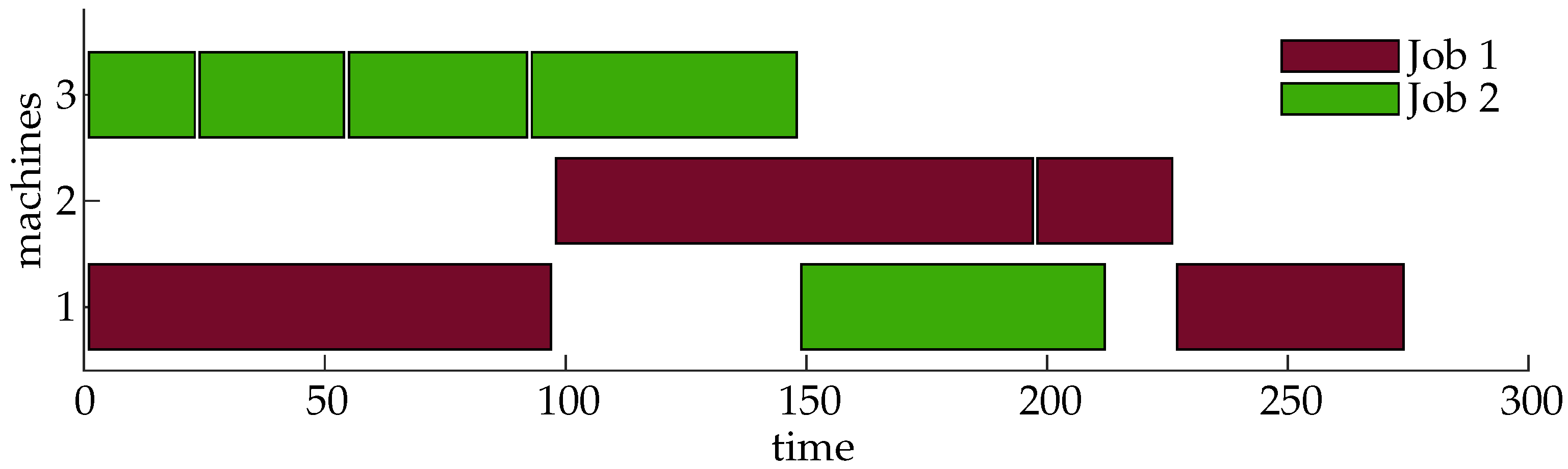
5. Numerical Examples

In order to illustrate the applicability of the MPC scheme presented in Section 4, we simulate one small- and one medium-sized scheduling problem from literature. From the set of problems used by Lunardi et al. [37] for evaluating their methods we select “sops1.json” and “mops1.json”, which can be found at https://willtl.github.io/ops (accessed on 20 August 2021). As we do not consider all effects that are handled by Lunardi et al. [37], we omit some particularities and only simulate the scheduling problems in the form described in Section 2. To arrive at this description, the JSON files are parsed with a simple Matlab script and the relevant information are deduced. We consider the resource constraints (R5), meaning that not all machines can execute every task, and the precedence constraints (R1) among the tasks of the same job and the production times t P ( M , τ ) , which are already given as a number of production steps k P ( M , τ ) in the JSON files. From the problem description deduced from the JSON files, the Petri Net descriptions are generated with the Algorithms 1 and 2 implemented in Matlab, and their state space descriptions are used to formulate the MPC problems (16). For simulation of the manufacturing systems with the MPC in closed loop, we use Matlab R2019b on a ThinkPad L390 Yoga with an Intel® Core™i5-8265U CPU. As solver for the MILP (16) we use intlinprog, which is a standard solver for mixed integer linear programs in Matlab.
The problems are initialized with all tasks of all jobs being necessary and none of them being completed. As no cost function is given in the JSON file, we choose a linear cost function c ( x , u ) = c x x + c u u that weights every token in a starting places with 2, every token in a production places with 5, every token in a buffer places with 1, every token in a necessity places with 1, and every token in a completion places with 0. The cost of firing any transition is 1. This cost function fulfills the condition (18) for every operation O. In every starting state x O , S , a necessity place is marked with one token, and in every resulting state x O , C that can be reached by executing the operation O through firing a transition u T U O , S , this token is moved to a completion place. This results in a cost decrease of c ( x O , S , 0 ) c ( x O , C , 0 ) = 1 between the states x O , S and x O , C . With Corollary 1, for every operation O there exists an extended prediction horizon N O + for which it is guaranteed to be completed. Therefore, if a sufficiently large extended prediction horizon N + is used, the MPC (16) is guaranteed to complete the production problem in closed loop according to Corollaries 2 and 3.
The small-sized scheduling problem “sops1.json” has n M = 3 machines, n τ = 9 tasks and n J = 2 jobs. The MPC (16) is parametrized with the prediction horizon N = 1 and the extended prediction horizon N + = 400 . The simulation time that the MPC needs to complete the scheduling problem “sops1.json” in closed loop is approximately 13 s and the resulting makespan is 274 time steps. The Gantt chart of the resulting closed loop schedule is given in Figure 4.
The medium-sized scheduling problem “mops1.json” has n M = 8 machines, n τ = 39 tasks and n J = 5 jobs. The MPC is parametrized with the prediction horizon N = 1 and the extended prediction horizon N + = 500 . It takes approximately 35 min to simulate the MPC in closed loop for the 786 time steps that it needs to complete the production problem. The Gantt chart of the closed loop schedule determined by the MPC is shown in Figure 5.
The simulation results are not directly comparable to the ones presented by Lunardi et al. [37]. We do not consider the particularities of their setup; we consider a different optimization criterion and additionally we simulate the production system in closed loop, meaning that we solve many different optimization problems, whereas Lunardi et al. [37] only determine one optimal schedule for the initial problem. The resulting average computation time of a single MPC optimization problem is slightly less than 50 milliseconds for the “sops1.json” and approximately 2.6 s for the “mops1.json”. Despite the fact that the cost function does not directly consider the makespan, the resulting closed loop schedule for the “sops1.json” has the makespan which Lunardi et al. [37] determined to be the shortest possible one. This illustrates how the production time is implicitly minimized under consideration of the given cost function as discussed at the end of Section 4.3. The presented examples are not designed to highlight the advantages of our approach, but they still illustrate that the MPC is applicable to common scheduling problems and that it neither has a particularly long computation time nor leads to a bad solution in the closed loop. In the next section we discuss the results and refer to further simplifications for the case of a linear cost function.

6. Discussion

In this section, we briefly summarize our results, discuss their advantages and limitations, and give an outlook on future work. In Section 2, we presented a general form of a scheduling problems for flexible manufacturing systems (FMSs). The problem is formulated as a job shop with multipurpose machines and sequence flexibility (JMPMSF), which generalizes various more specific problems used in literature on FMSs and thus has a wide range of potential applications. The restrictions and flexibilities of the JMPMSF are clearly stated in Section 2.1, and it is discussed in Section 2.3 how further restrictions lead to special cases that are more widely discussed, as for example the well-known job shop (JS) problem. The initial problem description is formulated in a modular way, which is motivated by the digital twins of the components in the manufacturing systems. It is assumed that the machines are cyber-physical production systems (CPPSs) and have a digital representation in the form of their digital twin that is synchronized in real-time. The CPPSs contribute their capabilities to the production system, where their abilities can be exploited. In the same way, the goods to be produced have a digital twin that holds instructions for their production. Thus, there are machine modules and product modules that need to be assigned to one another in the scheduling problem. This modularity is respected in the problem formulation in Section 2, and it is exploited for the automatic model generation in the form of a PN in Section 3 and in the analysis of the resulting scheduling problem in Section 4. By means of a PN formulation, the scheduling problem is formulated in an algebraic way that allows to apply methods from systems and control theory and specifically Model Predictive Control (MPC). In Section 5, we illustrate the applicability of the scheduling scheme with two simulation examples from literature.
The methodology is developed with respect to arbitrary scheduling objectives that can be formulated in the form of a cost function based on the elements in the manufacturing system. In this respect, one might think of the real material, energy, or storage cost that incur in the manufacturing system. In the resulting optimization problem, which is formulated to achieve the best possible performance with respect to the given objective, the value that accumulates over time with respect to the given cost function is minimized. The optimization is done with respect to a constant system model at first. However, under the assumption that changes are frequent in an FMS and thus the optimization for the far future might be futile, two measures are taken. On the one hand, the optimization is only conducted over a limited time horizon, and on the other hand, the optimization result is not blindly applied to the system, but only the actions planned for the current time instant. In order to determine the input, i.e., the manufacturing decisions, for the following time step, the current system state is measured and the optimization is conducted based on the true system state. The measurements are assumed to be readily available through the digital twins of the machines and products. By this, a feedback mechanism is introduced that naturally makes the scheduling strategy more robust and flexible than simply trying to apply an optimal open loop strategy. This general approach of MPC seems particularly suited under the assumption of frequent changes of FMSs in Industry 4.0.
The optimization problems (6) and (16) are MPC formulations for the scheduling of a given production problem in a JMPMSF provided in the form described in Section 2 and modeled as Petri Net. If the production problem is given, the MPC formulations can be parametrized such that the completion of the production problem is guaranteed by employing the results in Theorem 1 and the Corollaries 1–3. Those guarantees are obviously given with respect to the model of the system. However, due to the way they are determined, for the case of differences between the model and the real system, the controller will at least apply an input to the system and attempt to complete the scheduling problem. As long as disturbances and changes in the real system with respect to its initial model are perceived through measurements, they can be considered through the feedback mechanism. If they do not lead to the violation of the required assumptions and conditions, the guarantees are retained. Changes of this kind could be the breakdown of a machine, which is fed back by removing a token from the respective idle place in the Petri Net. As long as at least one of the other machines in the manufacturing system, which is still functional, can take over all the tasks of the broken machine, Assumption 2 is still true. If the precondition of Theorem 1 is still fulfilled for all operations taken over by another machine, the convergence guarantees can be retained or at least restored by adapting the prediction horizon N. Furthermore, changes in the cost function, which might be caused by decisions made on the management level or changing energy or material cost, can be handled as long as condition (8) in Theorem 1 is not violated. However, in order to retain the convergence guarantees of the proposed MPC schemes, a re-evaluation of the used prediction horizon N with respect to Theorem 1 is required.
Due to its modular structure, the model offers the possibility to include new jobs or new machines, as required in Section 2.2 and motivated by real production scenarios. This modularity is maintained through the model generation to the formulation of the control problem, and therefore it is easily possible to analyze whether the required properties are preserved despite changes in the problem description. The introduction of a new machine changes the convergence guarantees of the MPCs given with Theorem 1 and the Corollaries 1–3 only in exceptional cases. Generally, a new machine introduces further flexibility and thereby additional possibilities to perform manufacturing tasks in an efficient way without restricting existing ones. To be precise, it is unlikely that a new machine influences the production cost c P ( τ , M ) of a task τ on an existing machine M, or the relation between the cost of existing steady states x O , S and x O , C . If it is assumed that the properties of the existing parts of the production problem do not change, the introduction of a new machine does not change the convergence properties of the MPCs.
For the introduction of a new job J ^ , analogous arguments hold and the modular structure of the production problem can be exploited. Its completion can be guaranteed, by only analyzing the new job J ^ . First, for every task τ T J ^ of the new job it is investigated whether a smallest sufficient prediction horizon N O / N O + of the operation O = ( τ , J ^ ) can be found. If this is the case for all operations, a smallest sufficient prediction horizon N J ^ / N J ^ + of the new job can be computed according to Corollary 2. If this is smaller than the existing smallest sufficient prediction horizon N min / N min + , the convergence properties are preserved despite the new job. If N J ^ / N J ^ + is lager, the smallest sufficient prediction horizon can be adjusted accordingly. If necessary, the prediction horizon N or the extended prediction horizon N + needs to be extended to restore the convergence guarantee despite the new job.
The most challenging part in providing the convergence guarantees is certainly to determine the shortest sufficient prediction horizon N O / N O + , as for all states x O , S X O , S a corresponding state x O , C X O , C satisfying condition (8) needs to be found. Only then a value for N O / N O + can be computed based on the pair ( x O , S , x O , C ) . By exploiting Properties (P4), (P5) and (P8), the state x O , C can be characterized based on the state x O , S and the transitions in the PN description, as described in [18]. With this characterization, condition (8) can be expressed solely based on the steady state x O , S and an input vector u T U O , S , which only fires a single starting transition, without the need to determine the set X O , C
c ( x O , S , 0 ) > c ( x O , S B u T + A n B + u T , 0 ) .
Despite the slightly more restricting definition of the set X O , S in Definition 2 compared with [18], it might still be too large in practice such that it is practically impossible to check all conditions to prove the completion of a single operation. To make this endeavor feasible, we provided a condition for the case of a linear cost function c ( x , u ) = c x x + c u u in our previous work [18]. This is done by exploiting Property (P4) and the linearity of the cost function and thereby reducing the number of conditions to be investigated. For a given transition T, there are many possible steady states x O , S X O , S in which an input u T U O , S firing only the transition T can be applied without violating the non-negativity constraint (3). With the result in [18], instead of investigating all steady states x O , S X O , S , only one condition needs to be checked for each transition T with u T U O , S and thereby number of conditions to check is significantly reduced.
Due to linearity of the cost function, condition (19) reduces to
c x B u T > c x A n B + u T .
If this condition holds for at least one input u T U O , S , Theorem 1 and Corollary 1 can be used to conclude the existence of a smallest sufficient prediction horizon N O and N O + for operation O, respectively. As before, from the values of N O / N O + for every operation in the production problem the smallest sufficient prediction horizon N min / N min + that guarantees the completion of the production problem can be computed.
The conditions in Theorem 1 and Corollary 1 are only a sufficient conditions. This means that there might also be the possibility that the production problem will be completed by the MPCs (6) and (16) in case condition (8) is not satisfied. This would, for example, be the case if the execution of a single operation O cannot directly yield profit, and therefore does not satisfy condition (8), but it enables another operation O and the immediate execution of O after O satisfies condition (8), i.e., c ( x O , S , 0 ) > c ( x O , C , 0 ) . Such cases could be captured by also investigating sequences of operations with respect to condition (8) in Theorem 1 instead of only single operations.
The MPC optimization problems (6) and (16) formulated in Section 4 are designed for the solution of the scheduling problem presented in Section 2, which is known to be NP-hard. They are finite horizon approximations of the overall optimization problem that solves the whole scheduling problem until completion and therefore less computationally expensive. Nevertheless, their solution space still grows exponentially with the number of jobs and alternative machines. Thus, the computation of the optimal input trajectory u * ( · | k ) is computationally demanding. However, this optimization problem does not need to be solved completely in every time step. On the one hand, the last N 1 steps of the solution computed at time step k can be used as the first N 1 steps of a candidate solution at time step k + 1 as it is common in MPC [14]. As appending such a candidate solution with the input u ( N 1 | k + 1 ) = 0 is always feasible as shown in the proof of Lemma 3, a feasible solution of the optimization problem can be found instantaneously. On the other hand, also a suboptimal solution might be sufficient to complete the production problem, as we further discuss in Section 6.1.
We formulated the maximization of profitability of the manufacturing system as objective for the presented scheduling scheme in Section 2.2. We assume that it is possible to quantify the profitability with a cost function that can be used in the optimization problems (6) and (16). In practice, the formulation of a suitable cost function that represents the desired production goals is not an easy task. Even formulating scheduling objectives that are frequently used in literature, as, for example, the optimality criteria presented by Brucker [15], in the form of a stage cost function c ( x , u ) is not always trivial.
Compared with other scheduling schemes, we only consider a few of the possible restrictions in the scheduling problem. As we briefly mentioned at the end of Section 2.3, for example, the online printing shop considered by Lunardi et al. [37] is subject to further challenges, which we did not address and therefore also did not consider in the examples in Section 5. As stated in Remark 1, however, the consideration of further properties and constraints of a manufacturing system is possible in the presented setup, but requires adaptations of the employed algorithms. As an example, the explicit handling of waste can be considered through dedicated Petri Net structures in which waste products are generated during production and stored in specific buffers that need to be emptied from time to time. Discussing further possible extensions in detail and proving their properties is beyond the scope of this paper and the topic of future research.
In closely related literature, the solution of scheduling problems is considered as they are at some given time instant [16,25,29,35,36,37]. In contrast to that, we provide a strategy how to handle complex and possibly changing scheduling problems over the course of time. The analysis of the resulting closed loop is one of the contributions that distinguishes our work from existing approaches in literature.

6.1. Future Research Directions

In the presented approach, we focus on the solution of the scheduling problem by means of Model Predictive Control. The most important features are the guaranteed feasibility of the employed optimization problem and the guaranteed solution of the entire scheduling problem in closed loop in the sense of convergence to a state in which all tasks of all jobs are completed. The guarantee for recursive feasibility is directly given by the problem formulation. For the guarantee of the completion of operations in Theorem 1, it is assumed that the optimization performed during computation of the MPC control law is solved until the optimum. This assumption, however, is not needed for the guarantee of the completion of the production problem, which is already provided in Lemma 5 and based on a convergence property provided in Lemma 4. For the proofs of these Lemmas, the key criterion is that a non-zero input is applied to the system once it entered a steady state. If this property also holds for suboptimal solutions, the closed loop system will still converge to a state in which the production problem is completed. Under this mild assumption, the convergence guarantee for the optimal solution of the MPC optimization problem is retained also for suboptimal solutions. Therefore, if the optimal solution of the admittedly complex MPC optimization problems (6) and (16) cannot be found in the available amount of time, the MPC scheduling approach is still a viable solution technique for the initial scheduling problem. If an optimization algorithm is used which is able to return a suboptimal but feasible solution after a desired amount of time, the MPC scheduling approach provides the properties of a so called anytime MPC scheme. This means that it guarantees important properties of the closed loop system no matter how many iterations the optimization algorithm are performed [60]. On the other hand, the important arguments in the proofs are based on steady states, which by definition persist over time. Therefore, it can also be argued that the optimizer has enough time in the important cases such that the optimal solution is attained and the properties can be guaranteed despite the complexity of the optimization problem is high. Even if it is not required that the optimum is attained in the MPC optimization in order to guarantee convergence, an analysis of the closed loop performance is a possible future research direction. From MPC theory, it is known that the repeated solution of a finite horizon optimal control problem does generally not lead to the infinite horizon optimal solution [61]. Therefore, an analysis of the closed loop performance of the controlled system might yield interesting results.
The feedback mechanism itself introduces a certain amount of robustness against disturbances and changes in the system. However, as the growing demand for flexibility in Industry 4.0 might increases the uncertainty of the evolution of the manufacturing system, those effects might become even more relevant. Therefore, in future work, the robustness of the closed loop system can be rigorously analyzed, for example in terms of some assumed changes with respect to the initial manufacturing problem. Such changes might be machine dropouts or jobs that arrive during runtime and can be considered as disturbances. If the worst case disturbances are considered, methods form robust MPC can be applied, and if the disturbances are described probabilistically, the problem falls into the domain of stochastic MPC [14]. Especially with respect to machine dropouts, where the worst case scenarios are overly conservative, the consideration of a dropout probability is promising. In this case, stochastic MPC minimizes the expected cost over the prediction horizon and thereby maximizes the expected profit in the manufacturing system.
The special case of a linear cost function was already briefly discussed in [18]. In a similar way, further classes of cost functions, for example, exhibiting certain separability conditions, can be analyzed. For the computation of the smallest sufficient prediction horizon that guarantees the completion of a given scheduling problem, specific algorithms can be formulated, which exploit the special characteristics of the cost function to simplify the computation. With respect to further special cases, more restrictive scheduling problems as, for example, the job shop, the flow shop or the open shop can be investigated. Furthermore, the discussion how the different job characteristics presented by Brucker [15] or further challenges as the particularities in the online printing shop considered by Lunardi et al. [37] can be integrated in our framework is an interesting future topic. Finally, real-world problems with relevant scheduling objectives can be the subject of further research.
Motivated by the potential further increase in flexibility and the trend towards CPPSs, the modular structure of the problem setup and the deduced model can be further exploited. The model generated in Section 3 from the problem setup described in Section 2 basically consists of separate processes for each job that are linked via idle places of the machines. From this structure, an agent-based approach, similar to the one presented by Xiang and Lee [62] for a scheduling problem, can be developed or the problem can be formulated in the form of a distributed MPC problem [63]. One possible approach would be to consider product agents for every job. The product agents then solve their local optimization problem and compete with each other for the machines. This requires coordination between the agents in order to arrive at an optimal production schedule. Depending on the interaction mechanism, this leads to a distributed optimization problem that approximates the centralized optimization problems used in the MPC problems (6) and (16). The smaller individual optimization problems will be easier to solve, but the global optimal solution might only be obtained in special cases and potentially only after multiple iterations between the competing agents [63].

7. Conclusions

Motivated by the changes through the implementation of Industry 4.0, we developed a novel scheduling scheme for flexible manufacturing system that is based on Model Predictive Control. The initial problem formulation of a job shop with multipurpose machines and sequence flexibility captures a wide class of relevant scheduling problems. This generality allows the direct application of the presented methods on a variety of important special cases. The initial scheduling problem is then automatically transformed into a Petri Net formulation, which we slightly adapted to better suit its purpose as basis for the feedback control mechanism that we use for scheduling. This transformation mechanism serves as a blueprint that can be adapted to similar problem descriptions in order to bring them into a form that allows the application of control theoretic tools. The production schedule is generated with MPC, where the cost of the production process is explicitly considered. The MPC formulation allows to rigorously prove the completion of the initial scheduling problem in closed loop based on verifiable conditions on the elements involved. Due to the feedback mechanism that is inherent in MPC, the scheduling scheme can react to changes in the problem setup and to exploit the flexibility of the manufacturing system.
The presented approach can serve as a general guideline on how to automatically transform complex scheduling problems into a form in which MPC can be applied. The presented solution only considers a part of the properties that need to be taken into account in production planning and scheduling but it has the potential to be enhanced and adapted in order to include further criteria. Furthermore, in those cases, the possibility to provide proven guarantees based on the MPC problem formulation will be a significant advantage.

Author Contributions

Conceptualization, P.W. and F.A.; methodology, P.W. and F.A.; formal analysis, P.W.; investigation, P.W.; writing—original draft preparation, P.W.; writing—review and editing, P.W. and F.A.; visualization, P.W.; supervision, F.A.; project administration, F.A.; funding acquisition, F.A. Both authors have read and agreed to the published version of the manuscript.

Funding

This work was supported by Deutsche Forschungsgemeinschaft (DFG, German Research Foundation) under Grant AL 316/12-2-279734922.

Institutional Review Board Statement

Not applicable.

Informed Consent Statement

Not applicable.

Data Availability Statement

Not applicable.

Conflicts of Interest

The authors declare no conflict of interest. The funders had no role in the design of the study; in the collection, analyses, or interpretation of data; in the writing of the manuscript; or in the decision to publish the results.

Appendix A

Proof of Lemma 1.
(P1)
We have to proof that there is no steady state ( x s , u s ) with u s 0 , u s N m . As no entry in u s can be negative, the effect of a positive entry in u s through B + can only be compensated by the effect of a positive entry in u s through B , and vice versa. In the same sense the effect that an input arc ( P , T ) has when the transition T fires in the firing count vector u s can only be reversed by an output arc ( T , P ) of a transition T in u s . Note that T = T would be possible. To prove that there is no steady state ( x s , u s ) with u s 0 can be verified by noticing that only starting transitions T ( , S ) are handled in the controlled part of the PN T C . Every starting transition has an input arc ( P ( 0 , · , · , N ) , T ( , S ) ) from a necessity place P ( 0 , · , · , N ) and its effect cannot be reverted, since there is no arc back to the necessity places from any other transition.
(P2)
For this property, the independent part T I of the PN has to be considered, as it influences the matrix A which is relevant to characterize steady states. A state x s is a steady state, if and only if no place P is marked that is an input place of a transition T T I ; otherwise, the automatic firing of the transition T would move the tokens from P according to the arcs connected to T. (A transition which only has a trivial loop from a single place P back to the same place is considered not to exist as it does not have any effect.) In the state space form this happens through the multiplication A x s . As all production transitions T ( , P ) and finishing transitions T ( , F ) are handled in the independent part, none of their input places is allowed to be marked in a steady state x s . As every production place P ( , P ) is either input place of a production- or finishing transition, none of them is allowed be marked in a steady state. Through the Property (I1), the reverse direction is true as well.
(P3)
The initial state x 0 is a vector of natural numbers, i.e., x 0 N n , as in Algorithm 1 the places are only marked with one token or they are not marked at all. That x 0 is a steady state follows directly from Property (P2) and by noticing that in Algorithm 1 not production place is marked.
(P4)
Follows from the fact that A N n × n and simple algebraic arguments.
(P5)
If no production place is marked in the precondition x s = B u , it follows from Property (P2) that x s is a steady state. The preconditions of the controlled transitions T T C constitute their input places. As only starting transitions T ( , S ) are in the set T C , only the input places of the starting transitions need to be considered. Due to Property (P2) and as no production place P ( , P ) is an input place to a starting transitions, the Property (P5) is true.
(P6)
A task τ is completed if its completion place P ( 0 , τ , J , C ) is marked. A completion place is only input place to starting transitions. If a completion place is input place to some starting transitions T ( , S ) through an arc created in line 18 of Algorithm 2, it is also one of its output places through an arc created in the same line and the weight of both arcs is the same.
(P7)
This follows directly from A being a matrix of natural numbers, i.e., A N n × n .
(P8)
First note that all finishing transitions T ( , F ) mark an idle place P ( · , 0 , 0 , I ) , a buffer place P ( , B ) and a completion place P ( 0 , · , · , C ) . All of those places only have starting transitions T ( , S ) as output transitions, which are all controlled. Thus, every finishing transition ends an independent firing sequence leading to it. As every production sequence ultimately ends with a finishing transition after k P steps, every production sequence terminates and a steady state is reached. In the matrix A, this is represented as a shifting sequence which ends in a state x ¯ = A k ¯ x , in which and entry x ¯ i with x i I D = ( M , τ , J , P k P ) is marked. Multiplying x ¯ with A, the entry x i is multiplied with the i-th column of A, which corresponds to the finishing transition T ( , F ) being the output transition of P ( M , τ , J , P k P ) , as described in Section 3.2. After this multiplications a state x s is reached in which only entries corresponding to places without independent output transitions are marked, i.e., idle places P ( · , 0 , 0 , I ) , buffer places P ( , B ) and completion places P ( 0 , · , · , C ) . Therefore, the diagonal entries corresponding to them are left unchanged and no entries are added to the respective columns in the process of generating the matrix A form the Petri Net. Multiplying the resulting vector x s with A once again does not change those entries in x s any more. This holds for all production sequences and the system ultimately enters a steady state with x s = A x s .
(P9)
To proof this property we have to analyze the input places that correspond to the starting transitions T ( · , τ , J , S ) of the investigated operation O = ( τ , J ) . Those all have the necessity place P ( 0 , τ , J , N ) and the completion places P ( 0 , τ , J , C ) of all τ T τ as common input places. P ( 0 , τ , J , N ) will remain marked until one of the starting transition was fired and task τ was executed. The places P ( 0 , τ , J , C ) will remain marked due to property (P6). For each of the investigated starting transitions, their remaining input places are one idle place P ( · , 0 , 0 , I ) and one buffer place P ( · , τ , J , B ) of another task τ of the same job J. In every steady state, the idle places of all machines P ( · , 0 , 0 , I ) are marked and thus this holds for the steady states x s , 1 and x s , 2 . This is the case as only starting transitions remove tokens from the idle places and they inject them into a production sequence that ultimately leads back to the same idle place from which the token was removed. This happens through a completely independent sequence, i.e., a sequence which is completely represented in the matrix A (cf. Figure 3).
Now it needs to be shown that, in x x , 2 , at least one buffer place P ( · , τ , J , B ) is marked that has a starting transition T ( · , · , τ , τ , J , S ) of the investigated task τ as output transition, except the task τ already had been executed. It is known that one such buffer place was marked in the steady state x s , 1 , since otherwise τ could not have been started. This means that for the pair of tasks τ , τ the condition in line 13 of Algorithm 2 was true.
We now need to show that, if the task τ was not already executed, starting from the buffer place P ( · , τ , J , B ) only other buffer place P ( · , τ ¯ , J , B ) can be marked in any steady state x s , 2 , for which the condition in line 13 holds as well for the pair of tasks τ ¯ , τ and thus the transition T ( · , · , τ ¯ , τ , J , S ) is created to start τ .
Such a buffer place P ( · , τ ¯ , J , B ) can only be marked through a sequence that started with a starting transition T ( · , · , τ , τ ¯ , J , S ) , that was created in line 15 of Algorithm 2. Thus, for the pair τ , τ ¯ the condition in line 13 was true. If it is also true for the pair τ ¯ , τ , we found the buffer place P ( · , τ ¯ , J , B ) as the required one to start the task τ form x s , 2 through a transition T ( · , · , τ ¯ , τ , J , S ) .
Let us investigate the condition in line 13 for this pair step by step. The first statement in this condition ( τ ¯ τ ) is true since otherwise the task τ was just finished. The second statement in this condition ( τ T ¯ τ ¯ ) is true since otherwise the previous task τ ¯ could not have been started, since the task τ was not yet completed. The last statement in this condition ( { τ * T J : τ ¯ T ¯ τ * , τ * T ¯ τ } = ) is true as otherwise such a task τ * would not have allowed task τ to be started in x s , 1 , which we know was the case as stated in the precondition of Property (P9). This concludes the proof.

References

  1. Kagermann, H.; Helbig, J.; Hellinger, A.; Wahlster, W. Recommendations for Implementing the Strategic Initiative Industrie 4.0: Securing the Future of German Manufacturing Industry; Final Report of the Industrie 4.0 Working Group; Forschungsunion: Munich, Germany; Berlin, Germany, 2013. [Google Scholar]
  2. Rossit, D.A.; Tohmé, F.; Frutos, M. Industry 4.0: Smart Scheduling. Int. J. Prod. Res. 2019, 57, 3802–3813. [Google Scholar] [CrossRef]
  3. Negri, E.; Fumagalli, L.; Macchi, M. A review of the roles of digital twin in CPS-based production systems. Procedia Manuf. 2017, 11, 939–948. [Google Scholar] [CrossRef]
  4. Cohen, Y.; Naseraldin, H.; Chaudhuri, A.; Pilati, F. Assembly systems in Industry 4.0 era: A road map to understand Assembly 4.0. Int. J. Adv. Manuf. Technol. 2019, 105, 4037–4054. [Google Scholar] [CrossRef]
  5. Grieves, M. Digital Twin: Manufacturing Excellence Through Virtual Factory Replication; Technical Report; Florida Institute of Technology: Melbourne, FL, USA, 2014. [Google Scholar]
  6. Thomas, U.; Hirzinger, G.; Rumpe, B.; Schulze, C.; Wortmann, A. A New Skill Based Robot Programming Language Using UML/P Statecharts. In Proceedings of the IEEE International Conference on Robotics and Automation, Karlsruhe, Germany, 6–10 May 2013; pp. 461–466. [Google Scholar]
  7. Heim, R.; Nazari, P.M.S.; Ringert, J.O.; Rumpe, B.; Wortmann, A. Modeling Robot and World Interfaces for Reusable Tasks. In Proceedings of the IEEE/RSJ International Conference on Intelligent Robots and Systems (IROS), Hamburg, Germany, 28 September–2 October 2015; pp. 1793–1798. [Google Scholar] [CrossRef] [Green Version]
  8. Andersen, R.H.; Solund, T.; Hallam, J. Definition and Initial Case-Based Evaluation of Hardware-Independent Robot Skills for Industrial Robotic Co-Workers. In Proceedings of the ISR/Robotik 2014, 41st International Symposium on Robotics, Munich, Germany, 2–3 June 2014; pp. 1–7. [Google Scholar]
  9. Schlegel, C.; Lotz, A.; Lutz, M.; Stampfer, D.; Inglés-Romero, J.F.; Vicente-Chicote, C. Model-driven software systems engineering in robotics: Covering the complete life-cycle of a robot. It-Inf. Technol. 2015, 57, 85–98. [Google Scholar] [CrossRef]
  10. Wächter, M.; Ottenhaus, S.; Kröhnert, M.; Vahrenkamp, N.; Asfour, T. The armarx statechart concept: Graphical programing of robot behavior. Front. Robot. AI 2016, 3, 33. [Google Scholar] [CrossRef] [Green Version]
  11. Lindorfer, R.; Froschauer, R. Towards user-oriented programming of skill-based automation systems using a domain-specific meta-modeling approach. In Proceedings of the 2019 IEEE 17th International Conference on Industrial Informatics (INDIN), Helsinki, Finland, 22–25 July 2019; Volume 1, pp. 655–660. [Google Scholar] [CrossRef]
  12. Herrero, H.; Moughlbay, A.A.; Outón, J.L.; Sallé, D.; de Ipiña, K.L. Skill based robot programming: Assembly, vision and Workspace Monitoring skill interaction. Neurocomputing 2017, 255, 61–70. [Google Scholar] [CrossRef]
  13. Heuss, L.; Blank, A.; Dengler, S.; Zikeli, G.L.; Reinhart, G.; Franke, J. Modular Robot Software Framework for the Intelligent and Flexible Composition of Its Skills. In Advances in Production Management Systems. Production Management for the Factory of the Future; Springer: Cham, Switzerland, 2019; pp. 248–256. [Google Scholar] [CrossRef]
  14. Rawlings, J.B.; Mayne, D.Q.; Diehl, M.M. Model Predictive Control: Theory, Computation, and Design; Nob Hill Publishing: Madison, WI, USA, 2017. [Google Scholar]
  15. Brucker, P. Classification of Scheduling Problems. In Scheduling Algorithms; Springer: Berlin/Heidelberg, Germany, 2007; pp. 1–10. [Google Scholar] [CrossRef]
  16. Birgin, E.G.; Ferreira, J.E.; Ronconi, D.P. List scheduling and beam search methods for the flexible job shop scheduling problem with sequencing flexibility. Eur. J. Oper. Res. 2015, 247, 421–440. [Google Scholar] [CrossRef]
  17. Wenzelburger, P.; Allgöwer, F. A Petri Net Modeling Framework for the Control of Flexible Manufacturing Systems. IFAC-PapersOnLine 2019, 52, 492–498. [Google Scholar] [CrossRef]
  18. Wenzelburger, P.; Allgöwer, F. A Novel Optimal Online Scheduling Scheme for Flexible Manufacturing Systems. IFAC-PapersOnLine 2019, 52, 1–6. [Google Scholar] [CrossRef]
  19. Demir, Y.; İşleyen, S.K. Evaluation of mathematical models for flexible job-shop scheduling problems. Appl. Math. Model. 2013, 37, 977–988. [Google Scholar] [CrossRef]
  20. Genova, K.; Kirilov, L.; Guliashki, V. A survey of solving approaches for multiple objective flexible job shop scheduling problems. Cybern. Inf. Technol. 2015, 15, 3–22. [Google Scholar] [CrossRef] [Green Version]
  21. Chaudhry, I.A.; Khan, A.A. A research survey: Review of flexible job shop scheduling techniques. Int. Trans. Oper. Res. 2016, 23, 551–591. [Google Scholar] [CrossRef]
  22. Zhang, J.; Ding, G.; Zou, Y.; Qin, S.; Fu, J. Review of job shop scheduling research and its new perspectives under Industry 4.0. J. Intell. Manuf. 2019, 30, 1809–1830. [Google Scholar] [CrossRef]
  23. Türkyılmaz, A.; Şenvar, Ö.; Ünal, İ.; Bulkan, S. A research survey: Heuristic approaches for solving multi objective flexible job shop problems. J. Intell. Manuf. 2020, 31, 1949–1983. [Google Scholar] [CrossRef]
  24. Nasiri, M.M.; Kianfar, F. A hybrid scatter search for the partial job shop scheduling problem. Int. J. Adv. Manuf. Technol. 2011, 52, 1031–1038. [Google Scholar] [CrossRef]
  25. Birgin, E.G.; Feofiloff, P.; Fernandes, C.G.; De Melo, E.L.; Oshiro, M.T.I.; Ronconi, D.P. A MILP model for an extended version of the flexible job shop problem. Optim. Lett. 2014, 8, 1417–1431. [Google Scholar] [CrossRef] [Green Version]
  26. Beach, R.; Muhlemann, A.P.; Price, D.H.R.; Paterson, A.; Sharp, J.A. A review of manufacturing flexibility. Eur. J. Oper. Res. 2000, 122, 41–57. [Google Scholar] [CrossRef]
  27. Sethi, A.K.; Sethi, S.P. Flexibility in manufacturing: A survey. Int. J. Flex. Manuf. Syst. 1990, 2, 289–328. [Google Scholar] [CrossRef]
  28. Jain, A.; Jain, P.K.; Chan, F.T.S.; Singh, S. A review on manufacturing flexibility. Int. J. Prod. Res. 2013, 51, 5946–5970. [Google Scholar] [CrossRef]
  29. Kim, Y.K.; Park, K.; Ko, J. A symbiotic evolutionary algorithm for the integration of process planning and job shop scheduling. Comput. Oper. Res. 2003, 30, 1151–1171. [Google Scholar] [CrossRef]
  30. Pinedo, M.L. Deterministic Models: Preliminaries. In Scheduling: Theory, Algorithms, and Systems; Springer International Publishing: Cham, Switzerland, 2016; pp. 13–32. [Google Scholar] [CrossRef]
  31. Graham, R.L.; Lawler, E.L.; Lenstra, J.K.; Rinnooy Kan, A.H.G. Optimization and Approximation in Deterministic Sequencing and Scheduling: A Survey. In Discrete Optimization II; Annals of Discrete Mathematics; Hammer, P., Johnson, E., Korte, B., Eds.; Elsevier: Amsterdam, The Netherlands, 1979; Volume 5, pp. 287–326. [Google Scholar] [CrossRef] [Green Version]
  32. Hoos, H.H.; Stützle, T. Scheduling Problems. In Stochastic Local Search; Hoos, H.H., Stützle, T., Eds.; Morgan Kaufmann: San Francisco, CA, USA, 2005; Volume Chapter 9, pp. 417–465. [Google Scholar] [CrossRef]
  33. Brandimarte, P. Routing and scheduling in a flexible job shop by tabu search. Ann. Oper. Res. 1993, 41, 157–183. [Google Scholar] [CrossRef]
  34. Zubaran, T.K.; Ritt, M. An effective heuristic algorithm for the partial shop scheduling problem. Comput. Oper. Res. 2018, 93, 51–65. [Google Scholar] [CrossRef]
  35. Özgüven, C.; Özbakır, L.; Yavuz, Y. Mathematical models for job-shop scheduling problems with routing and process plan flexibility. Appl. Math. Model. 2010, 34, 1539–1548. [Google Scholar] [CrossRef]
  36. Vilcot, G.; Billaut, J.C. A tabu search and a genetic algorithm for solving a bicriteria general job shop scheduling problem. Eur. J. Oper. Res. 2008, 190, 398–411. [Google Scholar] [CrossRef]
  37. Lunardi, W.T.; Birgin, E.G.; Laborie, P.; Ronconi, D.P.; Voos, H. Mixed Integer linear programming and constraint programming models for the online printing shop scheduling problem. Comput. Oper. Res. 2020, 123, 105020. [Google Scholar] [CrossRef]
  38. Petri, C.A. Kommunikation mit Automaten. Ph.D. Thesis, Technischen Hochschule Darmstadt, Darmstadt, Germany, 1962. [Google Scholar]
  39. Seatzu, C.; Silva, M.; Van Schuppen, J.H. Control of Discrete-Event Systems; Springer: Berlin/Heidelberg, Germany, 2013; Volume 433. [Google Scholar] [CrossRef] [Green Version]
  40. Cassandras, C.G.; Lafortune, S. Introduction to Discrete Event Systems; Springer Science & Business Media: Berlin/Heidelberg, Germany, 2009. [Google Scholar] [CrossRef]
  41. Balduzzi, F.; Giua, A.; Menga, G. First-order hybrid Petri nets: A model for optimization and control. IEEE Trans. Robot. Autom. 2000, 16, 382–399. [Google Scholar] [CrossRef]
  42. Giua, A.; Seatzu, C. A systems theory view of Petri nets. In Advances in Control Theory and Applications; Bonivento, C., Marconi, L., Rossi, C., Isidori, A., Eds.; Springer: Berlin/Heidelberg, Germany, 2007; pp. 99–127. [Google Scholar] [CrossRef]
  43. Mahulea, C.; Giua, A.; Recalde, L.; Seatzu, C.; Silva, M. Optimal model predictive control of timed continuous Petri nets. IEEE Trans. Autom. Control 2008, 53, 1731–1735. [Google Scholar] [CrossRef] [Green Version]
  44. Júlvez, J.; Di Cairano, S.; Bemporad, A.; Mahulea, C. Event-driven model predictive control of timed hybrid Petri nets. Int. J. Robust Nonlinear Control 2014, 24, 1724–1742. [Google Scholar] [CrossRef]
  45. Taleb, M.; Leclercq, E.; Lefebvre, D. Model predictive control for discrete and continuous timed Petri nets. Int. J. Autom. Comput. 2018, 15, 25–38. [Google Scholar] [CrossRef]
  46. Recalde, L.; Teruel, E.; Silva, M. Autonomous continuous P/T systems. In International Conference on Application and Theory of Petri Nets; Springer: Berlin/Heidelberg, Germany, 1999; pp. 107–126. [Google Scholar] [CrossRef]
  47. Silva, M.; Recalde, L. On fluidification of Petri Nets: From discrete to hybrid and continuous models. Annu. Rev. Control 2004, 28, 253–266. [Google Scholar] [CrossRef]
  48. Lefebvre, D. Deadlock-free scheduling for timed Petri net models combined with MPC and backtracking. In Proceedings of the 2016 13th International Workshop on Discrete Event Systems (WODES), Xi’an, China, 30 May–1 June 2016; pp. 466–471. [Google Scholar] [CrossRef]
  49. Lefebvre, D. Dynamical scheduling and robust control in uncertain environments with Petri nets for DESs. Processes 2017, 5, 54. [Google Scholar] [CrossRef]
  50. Zhang, Q.; Liu, P.; Pannek, J. Modeling and predictive capacity adjustment for job shop systems with RMTs. In Proceedings of the 2017 25th Mediterranean Conference on Control and Automation (MED), Valletta, Malta, 3–6 July 2017; pp. 310–315. [Google Scholar] [CrossRef]
  51. Vargas-Villamil, F.D.; Rivera, D.E. A model predictive control approach for real-time optimization of reentrant manufacturing lines. Comput. Ind. 2001, 45, 45–57. [Google Scholar] [CrossRef]
  52. Cataldo, A.; Perizzato, A.; Scattolini, R. Production scheduling of parallel machines with model predictive control. Control Eng. Pract. 2015, 42, 28–40. [Google Scholar] [CrossRef]
  53. Köhler, P.N.; Müller, M.A.; Pannek, J.; Allgöwer, F. On Exploitation of Supply Chain Properties by Sequential Distributed MPC. IFAC-PapersOnLine 2017, 50, 7947–7952. [Google Scholar] [CrossRef]
  54. Subramanian, K.; Maravelias, C.T.; Rawlings, J.B. A state-space model for chemical production scheduling. Comput. Chem. Eng. 2012, 47, 97–110. [Google Scholar] [CrossRef]
  55. Subramanian, K.; Rawlings, J.B.; Maravelias, C.T.; Flores-Cerrillo, J.; Megan, L. Integration of control theory and scheduling methods for supply chain management. Comput. Chem. Eng. 2013, 51, 4–20. [Google Scholar] [CrossRef]
  56. Faulwasser, T.; Grüne, L.; Müller, M.A. Economic nonlinear model predictive control. Found. Trends® Syst. Control 2018, 5, 1–98. [Google Scholar] [CrossRef]
  57. Forbes, M.G.; Patwardhan, R.S.; Hamadah, H.; Gopaluni, R.B. Model predictive control in industry: Challenges and opportunities. IFAC-PapersOnLine 2015, 48, 531–538. [Google Scholar] [CrossRef]
  58. Müller, M.A.; Worthmann, K. Quadratic costs do not always work in MPC. Automatica 2017, 82, 269–277. [Google Scholar] [CrossRef]
  59. Alamir, M.; Bornard, G. Stability of a truncated infinite constrained receding horizon scheme: The general discrete nonlinear case. Automatica 1995, 31, 1353–1356. [Google Scholar] [CrossRef]
  60. Feller, C.; Ebenbauer, C. Sparsity-Exploiting Anytime Algorithms for Model Predictive Control: A Relaxed Barrier Approach. IEEE Trans. Control Syst. Technol. 2018, 28, 425–435. [Google Scholar] [CrossRef]
  61. Grüne, L.; Pannek, J. Nonlinear Model Predictive Control: Theory and Algorithms; Springer International Publishing: Cham, Switzerland, 2017. [Google Scholar]
  62. Xiang, W.; Lee, H.P. Ant colony intelligence in multi-agent dynamic manufacturing scheduling. Eng. Appl. Artif. Intell. 2008, 21, 73–85. [Google Scholar] [CrossRef]
  63. Maestre, J.M.; Negenborn, R.R. (Eds.) Distributed Model Predictive Control Made Easy; Springer: Berlin/Heidelberg, Germany, 2014; Volume 69. [Google Scholar] [CrossRef]
Figure 1. Elementary Petri Net structures in which the transitions can be assigned to the set of independent transitions T I .
Applsci 11 08145 g001
Figure 2. Elementary Petri Net structures in which the transitions must be actively controlled and always belong to the set of controlled transitions T C .
Applsci 11 08145 g002
Figure 3. Illustration of the production sequences for the execution of task τ of job J on machine M as it is generated in the Algorithms 1 and 2, with a = ( M , M , τ , τ , J ) and b = ( M , M , τ , τ , J ) . The tokens in the sequence are depicted as they are initialized in Algorithm 1. As at initialization no task τ or τ is already completed, the places P ( M , τ , J , B ) and P ( 0 , τ , J , C ) are not marked and the transition T ( M , M , τ , τ , J , S ) is not enabled.
Applsci 11 08145 g003
Figure 4. Gantt chart of the closed loop schedule for the small sized scheduling problem “sops1.json” [37], resulting from the application of the MPC (16).
Applsci 11 08145 g004
Figure 5. Gantt chart of the closed loop schedule for the medium sized scheduling problem “mops1.json” [37], resulting from the application of the MPC (16).
Applsci 11 08145 g005
Publisher’s Note: MDPI stays neutral with regard to jurisdictional claims in published maps and institutional affiliations.

