A Unified Approach for the Control of Power Electronics Converters. Part II: Tracking

Abstract

This paper extends the results recently proposed in Part I of this research work focused on the stabilization of power electronic converters. This second part is devoted to cases in which the underlying control problems can be translated into tracking control problems. This is the case for DC-AC converters whose output must track a sinusoidal reference signal. The idea is to tackle the problem in a unified manner in order to avoid as much as possible the use of approximations and to exploit all the mathematical properties of the corresponding switched models. The case in which measurable or non-measurable perturbations are present is considered. The proposed techniques are illustrated for two particular DC-AC converters simulated using the PSIM software.

1. Introduction

For many years, the control of power electronics converters has been a challenge for the control community [1,2,3]. Despite the fact that there has been renewed interest motivated by the increasing importance of renewable energies [4,5,6], the control problems associated with energy processing have been the main focus of the efforts of researchers because they possess several specific features that introduce significant difficulties into the underlying control problems of interest. Among the more stringent ones, we can highlight the switching nature combined with nonlinearities, present in almost all problems concerning energy conversion. Another motivation is related to the significant recent progress achieved in the domain of materials, electronic devices or components [7,8], but also in the control of switched or, more generally, hybrid systems [9,10], which have led to several new perspectives to deal with problems whose solutions cannot be easily obtained by the standard techniques.

A general model describing a large class of power converters is a bilinear differential model, whose state, composed of currents and voltages, belongs to a finite dimensional vector space, and control variables associated with the switched devices belong to a finite discrete set [1]. From this original model, it is possible to derive approximated models, such as an averaged model, which, although bilinear, exhibits constrained continuous control variables, allowing the use of all the methods developed for nonlinear systems (feedback linearization, sliding mode, flatness, passivity (see [11] and references therein)). It is also possible to linearize the averaged bilinear model around an equilibrium state and invoke the powerful robust linear control design techniques [12,13,14]. Among the numerous works, we can cite [15,16,17,18], where the problem is formulated in terms of a switched system whose modes are described by affine differential models and concern principally stabilization problems. Still in the context of stabilization problems, in [19], in which the original bilinear converter model is manipulated in such a way that allows it to exhibit a constant dynamical matrix (i.e., independent of the control variable), the authors show how to solve problems that cannot be easily solved when considering the original switched model.

When the objective is to enforce the output of the converter to follow a given periodic reference, the problem is more involved because it is formulated as a tracking problem [2] for which a solution with qualified properties such as stability and performance can be very difficult to obtain. Due to its importance, tracking control with disturbance rejection has been extensively studied in the control literature. If the reference signals are generated by an appropriate autonomous exosystem, the problem is known as the output regulation problem [20]. For linear systems, it has been solved in [21] from the solution of a set of algebraic matrix equations. Its extension to nonlinear systems involves the solution of a set of nonlinear differential equations, the Francis–Byrnes–Isidori equations, which allow the determination of an attractive invariant steady state. A few general works have been presented in the context of switched or hybrid control design methods. We can cite [22,23,24]. More closely related to the problem addressed in this paper, we can also cite [25], where the problem of nonlinear sliding mode output regulation is addressed. Using the concepts connected to the zero output tracking sub-manifold, a solution is proposed for nonlinear affine control systems with time-varying disturbance including both minimum and non-minimum phase systems extending some previous results proposed in [26,27,28,29] for minimum-phase systems, in [30,31] for linear systems, or in [32] for non-minimum-phase non-linear systems with a unitary relative degree. More closely related to the control of power converters, in [33], two closed-loop boost power converters are proposed for a DC-AC power conversion problem controlled using a sliding mode strategy. In [34], a cascade control scheme also based on sliding mode control is developed for the same boost inverter. One of the main difficulties is the non-minimum-phase property of such a converter, motivating the design of an indirect control law whose objective is to impose a tracking reference signal to the current inductors, the problem being then translated into the determination of an appropriate current reference signal. Several methods have been invoked for such a determination. In [35], a linearized internal dynamics is used, while in [36,37], the reference signal is obtained, respectively, by means of a uniform sequence of Galerkin’s approximations or from periodic solutions of Abel’s ordinary differential equation of the second kind. Several papers combining the previous approaches using sliding mode control or other nonlinear control techniques exist [38,39,40,41]. Recently, in [42], a solution for the half bridge inverter was proposed, and in [43], the case of the full bridge is considered using bipolar or unipolar strategies. The specificity of the aforementioned works is to formulate the control problems as tracking control problems directly for the switched models, seeking to extend the results of [21]. The specificity of the half-bridge and full-bridge inverters is that the dynamical matrix does not depend on the discrete control variable, drastically simplifying the resolution of the problem. For inverters whose dynamical matrix depends on the control variable, such as the boost inverter introduced in [33], the problem is more complicated and the method used in [42] cannot be directly extended. One of the main technical problems is to solve the set of algebraic matrix equations, which can be seen as an extension of the one in [21].

The main objective of this paper is to extend the approach proposed in [19], developed for stabilization problems, to the case of problems that can be formulated as tracking ones. As in [19], the idea is to derive formulations in a general setting and propose solutions that are justified and qualified from a theoretical point of view using efficient theoretical and numerical tools. In this sense, a crucial step consists of manipulating the original bilinear converter model in an appropriate way, leading to a model that is closely related to the switched model considered in the literature—for example, in [15] or [18]—but being better suited for solving control problems that cannot be easily solved when considering the original switched model. The approaches proposed in this paper could be easily extended in the context of the hybrid formulation paradigm proposed in [44] with the associated time and space regularization techniques. This extension is not considered and can be addressed in a future work. The paper is organized as follows. The next section recalls the main models considered in [19] and used in this work. In Section 3, the tracking problem is precisely stated and, in particular, the notion of admissible reference is defined. Section 4 develops a solution to the problem stated in Section 3, whose derivation is based on a central assumption discussed in detail. Section 5 considers the tracking problem in the presence of perturbations. Two cases are considered, the case in which the perturbations are not available for measurement and then not usable by the control law, and the case in which the perturbations are measurable using some low-cost sensors. In Section 6, the proposed methods are illustrated for two converters: the classical full-bridge inverter feeding nonlinear loads, and the boost inverter introduced in [33]. For this last case, the more involved determination of the state reference is discussed and obtained by two methods corresponding to the two means of controlling such a converter. The first one is obtained by the popular harmonic balance technique [45]. The second one justifies the development of a technique presented in Section 7, efficient when the dynamic of output reference is slow compared to the dynamic of the converter. The paper ends with the conclusions, proposing some extensions to be considered in future works.

Notations 1.

Throughout the paper, matrices of appropriate dimensions are denoted by capital letters. $\mathbb{R}$ denotes the set of real numbers. For a symmetric matrix P, $P<0(P\le 0)$ means that P is negative definite (negative semidefinite). $P>0$ means that symmetric matrix P is positive definite (i.e., $-P<0$). For matrices A and B, $A<B$ means that $A-B<0$. For a matrix A or a vector y, $A^T$ and $y^T$ denote their transposes. The Euclidian norm of a vector y is denoted by $\parallel y\parallel$. The matrix denoted by $diag(A_1,A_2\cdots ,A_N)$ is a block diagonal matrix whose diagonal blocks of appropriate dimensions are $A_1$, $A_2$, ⋯, $A_N$. I denotes the identity matrix of appropriate dimensions. $bi{n}_M\left(i\right)$ is the binary expression of i using M digits. The space of square integrable functions w is denoted by $L_2$ and ${\parallel w\parallel }_2^2={\int }_0^{\infty }w{\left(t\right)}^{T}w\left(t\right)dt$ is the associated 2-norm.

2. Preliminaries

In these preliminaries, the models considered in this paper, developed in detail in [19], are recalled. We consider systems described by

$$\left\{\begin{array}{ccc}\hfill {\displaystyle \frac{dx\left(t\right)}{dt}}& =& (A_0+A_{u_1\left(t\right)u_2\left(t\right)\cdots u_m\left(t\right)})x\left(t\right)+(B_0+B_{u_1\left(t\right)u_2\left(t\right)\cdots u_m\left(t\right)})v_{in}\left(t\right)\hfill \\ \hfill y\left(t\right)& =& (C_0+C_{u_1\left(t\right)u_2\left(t\right)\cdots u_m\left(t\right)})x\left(t\right)\hfill \end{array}\right.$$

(1)

where $x\left(t\right)\in {\mathbb{R}}^n$ is the state vector, $y\left(t\right)\in {\mathbb{R}}^p$ is the output vector and $u_i\left(t\right)\in \{0,1\}$ are the control variables. $v_{in}\left(t\right)\in {\mathbb{R}}^l$ is associated with a power source and, in many cases, it is constant. When this is the case, we replace $v_{in}\left(t\right)$ with $V_{in}$. $A_0,B_0,C_0$ are constant matrices of appropriate dimensions, and $A_0$ is supposed to be Hurwitz. The matrices ${•}_{u_1\left(t\right)u_2\left(t\right)\cdots u_m\left(t\right)},•=A,B,C$ are defined as

$${•}_{u_1\left(t\right)u_2\left(t\right)\cdots u_m\left(t\right)}=\sum _{i=1}^m{u}_i\left(t\right){•}_{u_i}$$

where ${•}_{u_i}$ are constant matrices of appropriate dimensions. It is also possible to write model (1) in an alternate form given by

$$\left\{\begin{array}{ccc}\hfill {\displaystyle \frac{dx\left(t\right)}{dt}}& =& (A_0+A_{\lambda \left(t\right)})x\left(t\right)+(B_0+B_{\lambda \left(t\right)})v_{in}\left(t\right)\hfill \\ \hfill y\left(t\right)& =& (C_0+C_{\lambda \left(t\right)})x\left(t\right)\hfill \end{array}\right.$$

(2)

where $\lambda \left(t\right)\in {\mathsf{\Lambda }}_S=\left\{\lambda \in {\left\{0,1\right\}}^M:\sum _{i=1}^M{\lambda }_i=1\right\}$ and

$${•}_{\lambda }\left(t\right)=\sum _{i=1}^{2^m}{\lambda }_i\left(t\right){•}_i,•=A,B,C$$

with ${•}_i={•}_{u_1\left(t\right)u_2\left(t\right)\cdots u_m\left(t\right)},•=A,B,C$ where $u_1\left(t\right)u_2\left(t\right)\cdots u_m\left(t\right)$ is the binary expression of $i-1$ denoted $bi{n}_M(i-1)$ [19]. The previous model can also be written in the following more compact form considered in the sequel:

$$\left\{\begin{array}{ccc}\hfill {\displaystyle \frac{dx\left(t\right)}{dt}}& =& A_{0}x\left(t\right)+B_0\left(x\left(t\right)\right)\lambda \left(t\right)\hfill \\ \hfill y\left(t\right)& =& C_{0}x\left(t\right)+D_0\left(x\left(t\right)\right)\lambda \left(t\right)\hfill \end{array}\right.$$

(3)

where, denoting $M=2^m$,

$$B_0\left(x\right)=\left[\begin{array}{ccc}{A}_{1}x+(B_0+B_1)v_{in}& \cdots & A_{M}x+(B_0+B_M)v_{in}\end{array}\right]$$

$$D_0\left(x\right)=\left[\begin{array}{ccc}{C}_{1}x& \cdots & C_{M}x\end{array}\right]$$

Another important model is that obtained by allowing the variable $\lambda \left(t\right)$ to belong to the set ${\mathsf{\Lambda }}_R=\{\lambda \in {\left[0,1\right]}^M:{\sum }_{i=1}^M{\lambda }_i=1\}$. The resulting model is known as the relaxed or embedded one [46]. In [46], it is shown that the initial value problem for (3) is dense in the solution set of initial value problems of the relaxed model for a topology ($C^0$-Whitney topology [47]) that is sufficiently general to cover almost all the associated practical problems of interest. In particular, this connection can be invoked for averaging or regularizing controls developed from (3) and applicable to the relaxed model using, for example, Pulse Width Modulation (PWM) or hysteresis comparators [19]. When $v_{in}\left(t\right)$ is constant, the classical concept of the equilibrium point is meaningless for systems described by (3). However, for the relaxed model, the classical notion of the equilibrium point is recovered and, because of the connection between the trajectories of (3) and the ones of its relaxed version, the set of equilibria for the relaxed model is of particular interest when considering model (3). This interest can be discussed in terms of refining the notion of the “solution” for model (3) (Caratheodory, Filippov’s solutions, etc.—see [48] for details). In this context, the set of equilibrium points associated with (3) is given by

$$X_{eq}=\left\{x_e\in {\mathbb{R}}^n,{\lambda }_e\in {\mathsf{\Lambda }}_R:A_0{x}_e+B_0\left(x_e\right){\lambda }_e=0\right\}$$

Under an appropriate invertibility condition, an alternate expression is

$$X_{eq}=\left\{x_e\in {\mathbb{R}}^n,{\lambda }_e\in {\mathsf{\Lambda }}_R:x_e=-{\left[\sum _{i=1}^M{\lambda }_{ei}(A_0+A_i)\right]}^{-1}\left[\sum _{i=1}^M{\lambda }_{ei}(B_0+B_i)\right]V_{in}\right\}$$

3. Problem Statement

The problem addressed in this paper is to enforce the output to track a given reference. The problem is known in the literature as the output regulation problem when the reference is generated by a neutrally stable exosystem described by [20]

$${\displaystyle \frac{dz}{dt}}=\mathsf{\Theta }\left(z\right),z\left(0\right)=z_0$$

(4)

where $z\left(t\right)\in {\mathbb{R}}^s$. Under this assumption, the reference $x_{ref}$ is expressed by

$$x_{ref}={\mathsf{\Pi }}_1\left(z\right)$$

where ${\mathsf{\Pi }}_1\left(0\right)=0$. Define the set of reference signals

$$X_{ref}=\left\{x_{ref}:{\mathbb{R}}_{+}\to {\mathbb{R}}^n:x_{ref}={\mathsf{\Pi }}_1\left(z\right) \mathrm{and} \dot{z}=\mathsf{\Theta }\left(z\right),z\left(0\right)=z_0,z_0\in {\mathbb{R}}^s\right\}$$

If $\dot{z}=0,z\left(0\right)=K\in \mathbb{R}$ and

$$x_{ref}={\mathsf{\Pi }}_1\left(z\right)=-{\displaystyle \frac{1}{K}}{\left[\sum _{i=1}^M{\lambda }_{ei}(A_0+A_i)\right]}^{-1}\left[\sum _{i=1}^M{\lambda }_{ei}(B_0+B_i)\right]V_{in}z,{\lambda }_e\in {\mathsf{\Lambda }}_R$$

then $X_{ref}=X_{eq}$. This means that the stabilization problem solved in [19] is a particular case of a tracking problem. From a practical point of view, not all the reference signals can be followed by a given converter. In general, the converter is designed to follow a specific set of signals referred to as admissible. To define the structure of the set of such signals, define the following map:

$${\mathsf{\Pi }}_2\left(z\right)=-A_0{\mathsf{\Pi }}_1\left(z\right)+{\displaystyle \frac{\partial {\mathsf{\Pi }}_1}{\partial z}}\mathsf{\Theta }\left(z\right)$$

(5)

Definition 1. 

A reference signal is said to be admissible if it belongs to the following set:

$$X_{Ad}=\left\{x_{ref}\in X_{ref},\exists {\lambda }_{ref}:\mathbb{R}\to {\mathsf{\Lambda }}_R:{\mathsf{\Pi }}_2\left(z\right)=B_0\left(x_{ref}\right){\lambda }_{ref}\right\}$$

In other words, from (5), we have

$${\displaystyle \frac{\partial {\mathsf{\Pi }}_1}{\partial z}}\mathsf{\Theta }\left(z\right)=A_0{\mathsf{\Pi }}_1\left(z\right)+{\mathsf{\Pi }}_2\left(z\right)$$

From the admissibility of the reference signal, we deduce that there exists ${\lambda }_{ref}:\mathbb{R}\to {\mathsf{\Lambda }}_R$ such that

$${\displaystyle \frac{\partial {\mathsf{\Pi }}_1}{\partial z}}\mathsf{\Theta }\left(z\right)=A_0{\mathsf{\Pi }}_1\left(z\right)+B_0\left({\mathsf{\Pi }}_1\left(z\right)\right){\lambda }_{ref}$$

(6)

which is nothing but

$${\dot{x}}_{ref}=A_0{x}_{ref}+B_0\left(x_{ref}\right){\lambda }_{ref}$$

Equation (6) is known as a regulator equation and the existence of ${\mathsf{\Pi }}_1\left(z\right)$ and ${\lambda }_{ref}$ is a necessary condition for the solvability of the tracking control problem (see [25]). We introduce the tracking error signal

$$e\left(t\right)=x\left(t\right)-x_{ref}\left(t\right)=x\left(t\right)-{\mathsf{\Pi }}_1\left(z\right)\left(t\right)$$

Then, we have

$$\begin{array}{cc}\hfill \frac{de\left(t\right)}{dt}& =\frac{dx\left(t\right)}{dt}-{\displaystyle \frac{\partial {\mathsf{\Pi }}_1}{\partial z}}\mathsf{\Theta }\left(z\right)\left(t\right)\hfill \\ \hfill & =A_{0}x\left(t\right)+B_0\left(x\left(t\right)\right)\lambda \left(t\right)-{\displaystyle \frac{\partial {\mathsf{\Pi }}_1}{\partial z}}\mathsf{\Theta }\left(z\right)\left(t\right)\hfill \\ \hfill & =A_{0}e\left(t\right)+B_0\left(x\left(t\right)\right)\lambda \left(t\right)-{\mathsf{\Pi }}_2\left(z\right)\left(t\right)\mathrm{from}\left(5\right)\hfill \end{array}$$

(7)

The tracking problem can now be precisely stated.

Problem 1. 

Design a control law $\lambda :\mathbb{R}\to {\mathsf{\Lambda }}_S$ such that, for any initial condition $e\left(0\right)\in {\mathbb{R}}^n$, system (7) is globally asymptotically stable, ensuring that

$$\underset{t\to \infty }{lim}e\left(t\right)=0$$

4. Main Result

We suppose that $v_{in}\left(t\right)$ is constant and equal to $V_{in}$. Because the matrix $A_0$ is Hurwitz, there exist two positive definite matrices $P\in {\mathbb{R}}^{n\times n}$ and $Q\in {\mathbb{R}}^{n\times n}$ satisfying

$$A_0^{T}P+P{A}_0+2Q<0$$

(8)

To solve the previous problem, we introduce an assumption that is quite similar to the one adopted in the context of the stabilization problem addressed in [19].

Assumption 1. 

Given an admissible reference signal $x_{ref}\in X_{Ad}$ and $x\left(t\right)\in {\mathbb{R}}^n$, there exist $\lambda \left(t\right)\in {\mathsf{\Lambda }}_R$ and a positive definite symmetric matrix $Q_1$, $0<Q_1\le Q$ such that, for all $t\ge 0$,

$$e^T\left(t\right)P\left[B_0\left(x\left(t\right)\right)\lambda \left(t\right)-{\mathsf{\Pi }}_2\left(z\right)\left(t\right)\right]\le -e^T\left(t\right)P{A}_{0}e\left(t\right)-e^T\left(t\right)Q_{1}e\left(t\right)$$

This assumption is central and it is important to note that it is satisfied for a large class of converters if matrices P and Q verify a condition stronger than (8), as stated in the following lemma.

Lemma 1. 

Suppose that there exist positive definite symmetric matrices $Q\in {\mathbb{R}}^{n\times n}$ and $S\in {\mathbb{R}}^{n\times n}$ such that

$${(A_0+A_i)}^{T}S+S(A_0+A_i)+2Q<0,i=1,\dots ,M$$

(9)

Then, Assumption 1 is satisfied, with P replaced by S.

Proof. 

Suppose that (9) satisfied. Then, for an admissible reference signal, there exists ${\lambda }_{ref}\left(t\right)$ such that $0\le {\lambda }_{ref}\left(t\right)\le 1$ and

$${\mathsf{\Pi }}_2\left(z\right)\left(t\right)=B_0(x_{ref}\left(t\right),{\lambda }_{ref}\left(t\right))\mathrm{for} \mathrm{all} t\ge 0$$

We have (time is omitted for convenience)

$$\begin{array}{cc}\hfill e^{T}S\left[B_0\left(x\right)\lambda -{\mathsf{\Pi }}_2\left(z\right)\right]& =e^{T}S[B_0\left(x\right)\lambda -B_0\left(x_{ref}\right){\lambda }_{ref}]\hfill \\ \hfill & =e^{T}S[B_0\left(x\right)(\lambda -{\lambda }_{ref})+\left[B_0\left(x\right)-B_0\left(x_{ref}\right)\right]{\lambda }_{ref}]\hfill \\ \hfill & =e^{T}S[B_0\left(x\right)(\lambda -{\lambda }_{ref})+\left[\begin{array}{ccc}{A}_{1}e& \cdots & A_{M}e\end{array}\right]{\lambda }_{ref}]\hfill \\ \hfill & =e^{T}S{B}_0\left(x\right)(\lambda -{\lambda }_{ref})+e^{T}S\sum _{i=1}^M{\lambda }_{{ref}_i}(A_0+A_i)e-e^{T}S{A}_{0}e\hfill \end{array}$$

For $\lambda ={\lambda }_{ref}$, we have

$$e^{T}S{A}_{0}e+e^{T}S[B_0\left(x\right){\lambda }_{ref}-B_0\left(x_e\right){\lambda }_{ref}])=e^{T}S\sum _{i=1}^M{\lambda }_{e_{{ref}_i}}(A_0+A_i)e<-e^{T}Qe$$

from (9). By continuity arguments, for all $t>0$ fixed, there always exists a neighborhood of ${\lambda }_{ref}\left(t\right)$ such that

$$e^{T}S{A}_{0}e+e^{T}S[B_0\left(x\right)\lambda -B_0\left(x_{ref}\right){\lambda }_{ref}])=e^{T}S\sum _{i=1}^M{\lambda }_{{ref}_i}(A_0+A_i)e+e^{T}S{B}_0\left(x\right)(\lambda -{\lambda }_{ref})<-e^{T}Qe$$

Then, Assumption 1 is satisfied for P replaced with S and the proof is complete. □

If the conditions of Lemma 1 are satisfied, this means that the set of matrices $A_0+A_i$ is a set of quadratically stable matrices [49]. From the above assumption, another important lemma can be deduced.

Lemma 2. 

If Assumption 1 is satisfied, we have

$$\begin{array}{ccc}\hfill {\displaystyle \underset{\lambda \in {\mathsf{\Lambda }}_S}{min}{e}^T\left(t\right)P\left[A_{0}e\left(t\right)+B_0\left(x\left(t\right)\right)\lambda -{\mathsf{\Pi }}_2\left(z\right)\left(t\right)\right]}& \le & -e^T\left(t\right)Q_{1}e\left(t\right)\hfill \end{array}$$

Proof. 

Suppose that the reference signal is admissible; we have by convexity

$$\begin{array}{cc}\hfill & \underset{\lambda \in {\mathsf{\Lambda }}_S}{min}{e}^T\left(t\right)P\left[A_{0}e\left(t\right)+B_0\left(x\left(t\right)\right)\lambda -{\mathsf{\Pi }}_2\left(z\right)\left(t\right)\right]\hfill \\ \hfill & =\underset{\lambda \in {\mathsf{\Lambda }}_R}{min}{e}^T\left(t\right)P\left[A_{0}e\left(t\right)+B_0\left(x\left(t\right)\right)\lambda -{\mathsf{\Pi }}_2\left(z\right)\left(t\right)\right]\hfill \\ \hfill & =e{\left(t\right)}^{T}P{A}_{0}e\left(t\right)+\underset{\lambda \in {\mathsf{\Lambda }}_R}{min}e{\left(t\right)}^{T}P\left[B_0\left(x\left(t\right)\right)\lambda -{\mathsf{\Pi }}_2\left(z\right)\left(t\right)\right]\hfill \\ \hfill & \le -e{\left(t\right)}^T{Q}_{1}e\left(t\right)\mathrm{by}\mathrm{Assumption}1\hfill \end{array}$$

□

The main result of this section can now be stated.

Theorem 1. 

Consider system (3) with an admissible reference signal described by the exosystem (4) and suppose that Assumption 1 is satisfied. Then, the control $\lambda \left(t\right)$ defined by

$$\lambda \left(t\right)=arg\left\{\underset{d\in {\mathsf{\Lambda }}_S}{min}{e}^T\left(t\right)P\left[A_{0}e\left(t\right)+B_0\left(x\left(t\right)\right)d-{\mathsf{\Pi }}_2\left(z\right)\left(t\right)\right]\right\}=arg\left\{\underset{d\in {\mathsf{\Lambda }}_S}{min}{e}^T\left(t\right)P{B}_0\left(x\left(t\right)\right)d\right\}$$

solves Problem 1. In addition, the tracking error satisfies

$$J\left(e\right)={\int }_0^{\infty }{e}^T\left(t\right)Q_{1}e\left(t\right)dt\le \frac{1}{2}{e}^T\left(0\right)Pe\left(0\right)$$

(10)

Proof. 

Consider the Lyapunov function $V\left(e\left(t\right)\right)=\frac{1}{2}{e}^T\left(t\right)Pe\left(t\right)$. Then,

$$\begin{array}{cc}\hfill \frac{dV\left(e\right(t\left)\right)}{dt}& =e{\left(t\right)}^{T}P\frac{de\left(t\right)}{dt}=e{\left(t\right)}^{T}P\left(A_{0}e\left(t\right)+B_0\left(x\left(t\right)\right)\lambda \left(t\right)-{\mathsf{\Pi }}_2\left(z\right)\left(t\right)\right)\hfill \end{array}$$

$$\begin{array}{cc}\hfill & =\underset{d\in {\mathsf{\Lambda }}_S}{min}\left[e{\left(t\right)}^{T}P(A_{0}e\left(t\right)+B_0\left(x\left(t\right)\right)d-{\mathsf{\Pi }}_2\left(z\right)\left(t\right)\right]\hfill \end{array}$$

(11)

$$\begin{array}{cc}\hfill & \le -e{\left(t\right)}^T{Q}_{1}e\left(t\right)\mathrm{by}\mathrm{Lemma}2\hfill \end{array}$$

Since ${\displaystyle \frac{dV\left(e\right)}{dt}}\le -{\lambda }_{min}\left(Q_1\right){\parallel e\parallel }^2$ for all $e\ne 0$, and because, at the instants of jumps $t_j$, we have $e\left(t_j^{-}\right)=e\left(t_j^{+}\right)$, we conclude that $\underset{t\to \infty }{lim}e\left(t\right)=0$. Now, integrating (11), from zero to infinity, and taking into account that $V\left(e\right(\infty \left)\right)=0$ and $V\left(e\left(t_j^{-}\right)\right)=V\left(e\left(t_j^{+}\right)\right)$, we obtain (10).

□

5. Tracking with Perturbations

When the system is affected by external perturbations, the previous approach can be extended to reject them. Model (1) is modified accordingly in order to consider the effects of perturbations. It is expressed as

$$\left\{\begin{array}{ccc}\hfill {\displaystyle \frac{dx\left(t\right)}{dt}}& =& (A_0+A_{u_1\left(t\right)u_2\left(t\right)\cdots u_m\left(t\right)})x\left(t\right)+(B_0+B_{u_1\left(t\right)u_2\left(t\right)\cdots u_m\left(t\right)})v_{in}\left(t\right)+(E_0+E_{u_1\left(t\right)u_2\left(t\right)\cdots u_m\left(t\right)})w\left(t\right)\hfill \\ \hfill y\left(t\right)& =& (C_0+C_{u_1\left(t\right)u_2\left(t\right)\cdots u_m\left(t\right)})x\left(t\right)+(F_0+F_{u_1\left(t\right)u_2\left(t\right)\cdots u_m\left(t\right)})w\left(t\right)\hfill \end{array}\right.$$

(12)

where $w\left(t\right)\in {\mathbb{R}}^r$, $w\in L_2$ is the perturbation. The matrices $E_0$, $E_{u_1\left(t\right)u_2\left(t\right)\cdots u_m\left(t\right)}$, $F_0$ and $F_{u_1\left(t\right)u_2\left(t\right)\cdots u_m\left(t\right)}$ are defined similarly as in Section 2. Following the developments of Section 2, we can obtain an augmented model written as

$$\left\{\begin{array}{c}{\displaystyle \frac{dx\left(t\right)}{dt}}=A_{0}x\left(t\right)+B_0\left(x\left(t\right)\right)\lambda \left(t\right)+E_0\left(w\left(t\right)\right)\lambda \left(t\right)\hfill \\ y\left(t\right)=C_{0}x\left(t\right)+D_0\left(x\left(t\right)\right)\lambda \left(t\right)+F_0\left(w\left(t\right)\right)\lambda \left(t\right)\hfill \end{array}\right.$$

(13)

where, denoting $M=2^m$,

$$B_0\left(x\right)=\left[\begin{array}{ccc}{A}_{1}x+(B_0+B_1)v_{in}& \cdots & A_{M}x+(B_0+B_M)v_{in}\end{array}\right],E_0\left(w\right)=\left[\begin{array}{ccc}{E}_{1}w& \cdots & E_{M}w\end{array}\right]$$

$$D_0\left(x\right)=\left[\begin{array}{ccc}{C}_{1}x& \cdots & C_{M}x\end{array}\right],F_0\left(w\right)=\left[\begin{array}{ccc}{F}_{1}w& \cdots & F_{M}w\end{array}\right]$$

5.1. Rejection of Non-Measurable Perturbations

We begin with the case in which the perturbations are not available for measurement. In this case, it is not possible to use the knowledge of the perturbation in the controller structure. A means of measuring the rejection level of the perturbation is to consider the $L_2$ gain between the perturbation w and the signal of interest (here, the tracking error e) defined as [49]

$$\underset{{\parallel w\parallel }_2\ne 0}{sup}{\displaystyle \frac{{\parallel e\parallel }_2}{{\parallel w\parallel }_2}} \mathrm{where} {\parallel •\parallel }_2^2={\int }_0^{\infty }{•}^T•dt$$

We also recall that if there exists a function $V\left(x\right)$ and $\gamma \ge 0$, such that, for all t,

$${\displaystyle \frac{dV\left(x\right)}{dt}}+e^{T}e-{\gamma }^2{w}^{T}w<0$$

integrating the previous inequality between 0 and $T>0$ with $x\left(0\right)=0$, we can deduce that the $L_2$ gain is lower than or equal to $\gamma$ [49]. All the notations are in line with those in the previous section. The dynamic of the tracking error can be written as follows:

$$\begin{array}{cc}\hfill \frac{de\left(t\right)}{dt}& =\frac{dx\left(t\right)}{dt}-{\displaystyle \frac{\partial {\mathsf{\Pi }}_1}{\partial z}}\mathsf{\Theta }\left(z\right)\left(t\right)\hfill \\ \hfill & =A_{0}x\left(t\right)+B_0\left(x\left(t\right)\right)\lambda \left(t\right)+E_0(w\left(t\right)\lambda \left(t\right)-{\displaystyle \frac{\partial {\mathsf{\Pi }}_1}{\partial z}}\mathsf{\Theta }\left(z\right)\left(t\right)\hfill \end{array}$$

(14)

$$\begin{array}{cc}\hfill & =A_{0}e\left(t\right)+B_0\left(x\left(t\right)\right)\lambda \left(t\right)+E_0(w\left(t\right)\lambda \left(t\right)-{\mathsf{\Pi }}_2\left(z\right)\left(t\right)\mathrm{from}\left(5\right)\hfill \end{array}$$

(15)

The problem tackled here can be summarized as follows.

Problem 2. 

Design a control law $\lambda :\mathbb{R}\to {\mathsf{\Lambda }}_S$, such that, for any initial condition, $e\left(0\right)\in {\mathbb{R}}^n$, we have

(i) 

If $w\left(t\right)=0$, the tracking error is globally asymptotically stable, i.e.,

$$\underset{t\to \infty }{lim}e\left(t\right)=0$$

(ii) 

If $w\left(t\right)\ne 0$, for all $t>0$, the tracking error is bounded and the perturbation is rejected with a $L_2$ gain lower than $\gamma >0$, i.e., we have, for $e\left(0\right)=0$,

$${\parallel e\parallel }_2^2\le {\gamma }^2{\parallel w\parallel }_2^2$$

To solve Problem 2, we suppose that Assumption 1 is met and recall that it is the case for a large class of converters if P is replaced by a matrix satisfying the conditions of Lemma 1. However, to deal with the disturbance rejection problem, Assumption 1 must be refined.

Assumption 2. 

Given an admissible reference signal $x_{ref}\in X_{Ad}$ and $x\left(t\right)\in {\mathbb{R}}^n$, there exist $\lambda \left(t\right)\in {\mathsf{\Lambda }}_R$, a positive definite symmetric matrix $Q_1$ and a positive number γ such that, for all $\mu \left(t\right)\in {\mathsf{\Lambda }}_R$ and $t\ge 0$,

$$\begin{array}{c}\hfill e^T\left(t\right)P\left[B_0\left(x\left(t\right)\right)\lambda \left(t\right)+E_0\left(w\left(t\right)\right)\mu \left(t\right)-{\mathsf{\Pi }}_2\left(z\right)\left(t\right)\right]+e{\left(t\right)}^{T}e\left(t\right)-{\gamma }^{2}w{\left(t\right)}^{T}w\left(t\right)\\ \hfill \le -e^T\left(t\right)P{A}_{0}e\left(t\right)-e^T\left(t\right)Q_{1}e\left(t\right)\end{array}$$

It is important to note that this assumption is always satisfied for the class of converters satisfying the conditions of Lemma 1, as shown in the following one.

Lemma 3. 

Suppose that the conditions of Lemma 1 are met. Then, there exists a positive definite symmetric matrix $W\in {\mathbb{R}}^{n\times n}$ and a positive scalar δ such that

$$\left[\begin{array}{cc}{(A_0+A_i)}^{T}W+W(A_0+A_i)+2I& W{E}_j\\ E_j^{T}W& -2{\delta }^{2}I\end{array}\right]<0,i=1,\dots ,M;j=1,\dots ,M$$

(16)

Then, Assumption 2 is satisfied for $P=W$ and $\gamma =\delta$.

Proof. 

To show the first part of Lemma 3, suppose that the conditions of Lemma 1 are satisfied. Then, there exist positive definite symmetric matrices $Q\in {\mathbb{R}}^{n\times n}$ and $S\in {\mathbb{R}}^{n\times n}$ such that

$${(A_0+A_i)}^{T}S+S(A_0+A_i)+2Q<0,i=1,\dots ,M$$

(17)

Multiplying the previous inequalities by a positive scalar $\alpha >0$ such that $\alpha Q<I$, we can see that the matrix $W=\alpha S$ satisfies the inequalities

$${(A_0+A_i)}^{T}W+W(A_0+A_i)+2I<0,i=1,\dots ,M$$

(18)

and then there exists a positive number $\delta$ that is sufficiently large such that

$${(A_0+A_i)}^{T}W+W(A_0+A_i)+2I+{\displaystyle \frac{1}{2}}{\delta }^{-2}W{E}_j{E}_j^{T}W<0,i=1,\dots ,M,j=1,\dots ,M$$

which, by Schur complement [49], can be transformed into (16). To show the last part, suppose that (16) satisfied. Then, for any admissible reference signal, there exists ${\lambda }_{ref}\left(t\right)$ such that $0\le {\lambda }_{ref}\left(t\right)\le 1$ and

$${\mathsf{\Pi }}_2\left(z\right)\left(t\right)=B_0(x_{ref}\left(t\right),{\lambda }_{ref}\left(t\right))$$

We have (time is omitted for convenience)

$$\begin{array}{ccc}\hfill e^{T}W\left[B_0\left(x\right)\lambda +E_0\left(w\right)\mu -{\mathsf{\Pi }}_{2}z\right]& =& e^{T}W[B_0\left(x\right)+E_0\left(w\right)\mu +B_0\left(x_{ref}\right){\lambda }_{ref}]\hfill \\ & =& e^{T}W[B_0\left(x\right)(\lambda -{\lambda }_{ref})+E_0\left(w\right)\mu +\left(B_0\left(x\right)-B_0\left(x_{ref}\right)\right){\lambda }_{ref}]\hfill \\ & =& e^{T}W\left[E_0\left(w\right)\mu +B_0\left(x\right)(\lambda -{\lambda }_{ref})+\left[\begin{array}{ccc}{A}_{1}e& \cdots & A_{M}e\end{array}\right]{\lambda }_{ref}\right]\hfill \\ & =& {\displaystyle e^{T}W{E}_0\left(w\right)\mu +e^{T}W{B}_0\left(x\right)(\lambda -{\lambda }_{ref})+e^{T}W\sum _{i=1}^M{\lambda }_{{ref}_i}(A_0+A_i)e-e^{T}W{A}_{0}e}\hfill \end{array}$$

Using the fact that ${\lambda }_{ref}\in {\mathsf{\Lambda }}_R$ and $\mu \in {\mathsf{\Lambda }}_R$, we have

$$\begin{array}{cc}\hfill e^{T}W\left[B_0\left(x\right)\lambda +E_0\left(w\right)\mu -{\mathsf{\Pi }}_2\left(z\right)\right]& {\displaystyle ={\displaystyle \frac{1}{2}}\sum _{i=1}^M\sum _{j=1}^M{\lambda }_{e_{{ref}_i}}{\mu }_j\left[e^T{w}^T\right]\left[\begin{array}{cc}{(A_0+A_i)}^{T}W+W(A_0+A_i)+2I& W{E}_j\\ E_j^{T}W& -2{\delta }^{2}I\end{array}\right]\left[\begin{array}{c}e\\ w\end{array}\right]}\hfill \\ \hfill & +e^{T}W{B}_0\left(x\right)(\lambda -{\lambda }_{ref})-e^{T}W{A}_{0}e+{\delta }^2{w}^{T}w-e^{T}e\hfill \\ \hfill & <-e^{T}e+{\delta }^2{w}^{T}w+e^{T}W{B}_0\left(x\right)(\lambda -{\lambda }_{ref})-e^{T}W{A}_{0}e\hfill \end{array}$$

from (16). For $\lambda ={\lambda }_{ref}$ and all $\mu \in {\mathsf{\Lambda }}_R$, we have

$$e^{T}W{A}_{0}e+e^{T}W[B_0\left(x\right){\lambda }_{ref}+E_0\left(w\right)\mu -B_0\left(x_e\right){\lambda }_{ref}])<-e^{T}e+{\delta }^2{w}^{T}w=-{\parallel e\parallel }_2^2+{\delta }^2{\parallel w\parallel }_2^2$$

By continuity arguments, for all $t>0$, there always exists a neighborhood of ${\lambda }_{ref}\left(t\right)$ and a positive definite matrix $Q_1$ such that

$$e^{T}W{A}_{0}e+e^{T}W[B_0\left(x\right)\lambda +E_0\left(w\right)\mu +B_0\left(x_{ref}\right){\lambda }_{ref}])+e^{T}e-{\delta }^2{w}^{T}w<-e^T{Q}_{1}e$$

Then, Assumption 2 is satisfied for P replaced by W and $\gamma$ by $\delta$. The proof is complete. □

To state the main result of this paragraph, we need the following result.

Lemma 4. 

If W and γ satisfy the conditions of Lemma 3, we have, for all $\mu \in {\mathsf{\Lambda }}_S$,

$$\begin{array}{ccc}& & {\displaystyle \underset{\lambda \in {\mathsf{\Lambda }}_S}{min}{e}^T\left(t\right)P\left[A_{0}e\left(t\right)+B_0\left(x\left(t\right)\right)\lambda +E_0\left(w\left(t\right)\right)\mu -{\mathsf{\Pi }}_2\left(z\right)\left(t\right)\right]}\hfill \\ & =& {\displaystyle \underset{\lambda \in {\mathsf{\Lambda }}_S}{min}{e}^T\left(t\right)P\left[A_{0}e\left(t\right)+B_0\left(x\left(t\right)\right)\lambda -{\mathsf{\Pi }}_2\left(z\right)\left(t\right)\right]+E_0\left(w\left(t\right)\right)\mu \le -e^T\left(t\right)Q_{1}e\left(t\right)-e{\left(t\right)}^{T}e\left(t\right)+{\gamma }^{2}w{\left(t\right)}^{T}w\left(t\right)}\hfill \end{array}$$

Proof. 

The proof follows by convexity arguments. □

A solution to Problem 2 is proposed in the following theorem.

Theorem 2. 

Consider system (13) with an admissible reference signal described by the exosystem (4) and suppose that Assumption 2 is satisfied. Then, the control $\lambda \left(t\right)$ defined by

$$\lambda \left(t\right)=arg\left\{\underset{d\in {\mathsf{\Lambda }}_S}{min}{e}^T\left(t\right)P\left[A_{0}e\left(t\right)+B_0\left(x\left(t\right)\right)d-{\mathsf{\Pi }}_2\left(z\right)\left(t\right)\right]\right\}=arg\left\{\underset{d\in {\mathsf{\Lambda }}_S}{min}{e}^T\left(t\right)P{B}_0\left(x\left(t\right)\right)d\right\}$$

solves Problem 2.

Proof. 

Consider the Lyapunov function $V\left(e\left(t\right)\right)=\frac{1}{2}{e}^T\left(t\right)Pe\left(t\right)$. Then,

$$\begin{array}{cc}\hfill \frac{dV\left(e\right(t\left)\right)}{dt}& =e{\left(t\right)}^{T}P\frac{de\left(t\right)}{dt}=e{\left(t\right)}^{T}P\left(A_{0}e\left(t\right)+B_0\left(x\left(t\right)\right)\lambda \left(t\right)+E_0\left(w\right)\lambda \left(t\right)-{\mathsf{\Pi }}_{2}z\left(t\right)\right)\hfill \end{array}$$

$$\begin{array}{cc}\hfill & =\underset{d\in {\mathsf{\Lambda }}_S}{min}\left[e{\left(t\right)}^{T}P(A_{0}e\left(t\right)+B_0\left(x\left(t\right)\right)d-{\mathsf{\Pi }}_2\left(z\right)\left(t\right)\right]+E_0\left(w\left(t\right)\right)\times arg\left\{\underset{d\in {\mathsf{\Lambda }}_S}{min}{e}^T\left(t\right)P{B}_0\left(x\left(t\right)\right)d\right\}\hfill \end{array}$$

(19)

$$\begin{array}{cc}\hfill & \le -e{\left(t\right)}^T{Q}_{1}e\left(t\right)-e{\left(t\right)}^{T}e\left(t\right)+{\gamma }^{2}w{\left(t\right)}^{T}w\left(t\right)\mathrm{by}\mathrm{Lemma}4\hfill \end{array}$$

We can deduce that

(i)

If $w=0$, since ${\displaystyle \frac{dV\left(e\right)}{dt}}\le -{\lambda }_{min}\left(Q_1\right){\parallel e\parallel }^2$ for all $e\ne 0$, and because, at the instants of jumps $t_j$, we have $e\left(t_j^{-}\right)=e\left(t_j^{+}\right)$, $\underset{t\to \infty }{lim}e\left(t\right)=0$.

(ii)

If $w\ne 0$, we have $\dot{V}\left(e\right)+e^{T}e-{\gamma }^2{w}^{T}w<0$. Integrating between $t=0$ and $t=T>0$, we deduce that

$${\displaystyle 0<V\left(e\left(T\right)\right)<V\left(e\left(0\right)\right)+{\gamma }^2{\int }_0^{T}w{\left(t\right)}^{T}w\left(t\right)dt-{\int }_0^{T}e{\left(t\right)}^{T}e\left(t\right)dt}$$

implying that the error $e(t$) is bounded because $w\in L_2$. In addition, when $T\to \infty$, we have ${\parallel e\parallel }_2^2<{\gamma }^2{\parallel w\parallel }_2^2+V\left(e\left(0\right)\right)$ and if $V\left(e\right(0\left)\right)=0$, then ${\parallel e\parallel }_2^2<{\gamma }^2{\parallel w\parallel }_2^2$, concluding the proof.

□

Introducing the change of variable $\beta ={\delta }^2$, it is possible to minimize $\gamma$ by solving the following LMI optimization problem: ${\displaystyle \underset{W>0}{min}\beta }$ under (16). Its optimal solution ${\beta }^{*}$ giving the optimal value of $\gamma$, ${\gamma }^{*}=\sqrt{{\beta }^{*}}$.

5.2. Rejection of Measurable Perturbations

Now, consider that perturbations are measurable. This case is of particular importance because, in many situations, it is possible to consider some external effects as measurable perturbations. For example, the variations in load or the DC input voltage can be available if some low-cost sensors are implemented. If $y_{ref}\left(t\right)$ is the associated output reference, we must have

$$y_{ref}\left(t\right)=C_0{x}_{ref}\left(t\right)+D_0\left(x_{ref}\left(t\right)\right){\lambda }_{ref}\left(t\right)+F_0\left(w\left(t\right)\right){\lambda }_{ref}\left(t\right)$$

where the state reference $x_{ref}\left(t\right)$ is admissible. As in the previous paragraph, the reference signal is generated from an exosystem (defined in exactly the same way), whose state belongs to a compact set ${\mathbb{R}}^s$ and is used to generate the state reference. However, the effects of the perturbation must be taken into account. This is why the state reference must include a term accounting for the perturbation. The state reference signal will be expressed as

$$x_{ref}\left(t\right)={\mathsf{\Pi }}_1\left(z\right)\left(t\right)+{\mathsf{\Pi }}_p\left(w\right)\left(t\right)$$

where ${\mathsf{\Pi }}_1$ and ${\mathsf{\Pi }}_p$ are appropriate maps, ${\mathsf{\Pi }}_1$ being defined as in the previous paragraph, and ${\mathsf{\Pi }}_p\left(0\right)=0$. The reference belongs to the following set:

$$X_{pert}=\left\{x_{ref}:{\mathbb{R}}_{+}\to {\mathbb{R}}^n:x_{ref}\left(t\right)={\mathsf{\Pi }}_1\left(z\right)\left(t\right)+{\mathsf{\Pi }}_p\left(w\right)\left(t\right)and\dot{z}\left(t\right)=\mathsf{\Theta }z\left(t\right),z\left(0\right)=z_0\in {\mathbb{R}}^s\right\}$$

A solution of the associated tracking control problem is only possible for admissible reference signals, the notion of admissibility being an extension of the one introduced in Section 3 and closely related to the signals that the converter is able to track in the presence of the measured perturbations.

Definition 2. 

For the system described by (13), a reference signal is said to be admissible if it belongs to the set

$$\begin{array}{c}\hfill X_{{Ad}_{pert}}=\left\{x_{ref}\in X_{pert}andw\in L_2:\exists {\lambda }_{ref}\left(t\right):\mathbb{R}\to {\mathsf{\Lambda }}_R:{\mathsf{\Pi }}_2(z,w)\left(t\right)=B_0\left(x_{ref}\left(t\right)\right){\lambda }_{ref}\left(t\right)\right.\\ \hfill \left.+E_0\left(w\left(t\right)\right){\lambda }_{ref}\left(t\right)\right\}\end{array}$$

where ${\mathsf{\Pi }}_2(z,w)=-A_0{\mathsf{\Pi }}_1\left(z\right)-A_0{\mathsf{\Pi }}_p\left(w\right)+{\displaystyle \frac{\partial {\mathsf{\Pi }}_1}{\partial z}}\mathsf{\Theta }\left(z\right)+{\displaystyle \frac{\partial {\mathsf{\Pi }}_p}{\partial w}}{\displaystyle \frac{dw}{dt}}$.

By the definitions of ${\mathsf{\Pi }}_2(z,w)$ and the set $X_{{Ad}_{pert}}$, we have

$${\displaystyle \frac{\partial {\mathsf{\Pi }}_1}{\partial z}}\mathsf{\Theta }\left(z\right)+{\displaystyle \frac{\partial {\mathsf{\Pi }}_p}{\partial w}}{\displaystyle \frac{dw}{dt}}=A_0\left[{\mathsf{\Pi }}_1\left(z\right)+{\mathsf{\Pi }}_p\left(w\right)\right]+{\mathsf{\Pi }}_2(z,w)$$

From the admissibility of $x_{ref}$, we deduce that $x_{ref}$ satisfies the following differential system, which can be seen as an extension of the regulator equation when measured perturbations are present.

$${\dot{x}}_{ref}=A_0{x}_{ref}+B_0\left(x_{ref}\right){\lambda }_{ref}+E_0\left(x_{ref}\right){\lambda }_{ref}$$

If $x_{ref}\left(t\right)\in X_{{Ad}_{pert}}$ and the error signal is defined as

$$e\left(t\right)=x\left(t\right)-x_{ref}\left(t\right)$$

we have

$$\begin{array}{cc}\hfill \frac{de\left(t\right)}{dt}& =A_{0}x\left(t\right)+B_0\left(x\left(t\right)\right)\lambda \left(t\right)+E_0\left(w\left(t\right)\right)\lambda \left(t\right)-{\displaystyle \frac{\partial {\mathsf{\Pi }}_1}{\partial z}}\mathsf{\Theta }\left(z\right)-{\displaystyle \frac{\partial {\mathsf{\Pi }}_p}{\partial w}}{\displaystyle \frac{dw}{dt}}\hfill \\ \hfill & =A_{0}e\left(t\right)+B_0\left(x\left(t\right)\right)\lambda \left(t\right)+E_0\left(w\left(t\right)\right)\lambda \left(t\right)-{\mathsf{\Pi }}_2(z,w)\left(t\right)\hfill \end{array}$$

(20)

Now, the problem can be precisely stated.

Problem 3. 

Design a control law $\lambda :\mathbb{R}\to {\mathsf{\Lambda }}_S$, such that, for any initial condition, $e\left(0\right)\in {\mathbb{R}}^n$, system (20) is globally asymptotically stable, ensuring that

$$\underset{t\to \infty }{lim}e\left(t\right)=0$$

Assumption 3. 

Given $x_{ref}\in X_{{Ad}_{pert}},x\left(t\right)\in {\mathbb{R}}^n$ and $w\left(t\right)\in {\mathbb{R}}^r$, there exist $\lambda \left(t\right)\in {\mathsf{\Lambda }}_R$ and a symmetric matrix $Q_1$, $0\le Q_1\le Q$ such that, for all $t\ge 0$

$$e^T\left(t\right)P\left[B_0\left(x\left(t\right)\right)\lambda \left(t\right)+E_0\left(w\left(t\right)\right)\lambda \left(t\right)-{\mathsf{\Pi }}_2(z,w)\left(t\right)\right]\le -e^T\left(t\right)P{A}_{0}e\left(t\right)-e^T\left(t\right)Q_{1}e\left(t\right)$$

It is important to note that if the conditions of Lemma 1 are satisfied, and this is a case for a large family of converters, for an admissible reference signal, Assumption 3 is met with $P=S$.

Lemma 5. 

Consider $x_{ref}\in X_{{Ad}_{pert}}$. Suppose that Assumption 3 is satisfied. Then,

$$\begin{array}{ccc}\hfill \underset{\lambda \in {\mathsf{\Lambda }}_S}{min}{e}^T\left(t\right)P\left[A_{0}e\left(t\right)+B_0\left(x\left(t\right)\right)\lambda +E_0\left(w\left(t\right)\right)\lambda -{\mathsf{\Pi }}_2(z,w)\left(t\right)\right]& \le & -e{\left(t\right)}^T{Q}_{1}e\left(t\right)\hfill \end{array}$$

Proof. 

Similar as for Lemma 2. □

Theorem 3. 

Consider the system (13) and $x_{ref}\in X_{{Ad}_{pert}}$. Suppose that Assumption 3 is satisfied. Then, the control $\lambda \left(t\right)$ defined by

$$\lambda \left(t\right)=arg\left\{\underset{d\in {\mathsf{\Lambda }}_S}{min}{e}^T\left(t\right)P[B_0\left(x\left(t\right)\right)+E_0\left(w\left(t\right)\right)]d\right\}$$

solves Problem 3. In addition, the tracking error satisfies

$$J\left(e\right)={\int }_0^{\infty }{e}^T\left(t\right)Q_{1}e\left(t\right)dt\le \frac{1}{2}{e}^T\left(0\right)Pe\left(0\right)$$

Proof. 

Consider the Lyapunov function $V\left(e\left(t\right)\right)=\frac{1}{2}{e}^T\left(t\right)Pe\left(t\right).$ Then,

$$\begin{array}{cc}\hfill \frac{dV\left(e\right(t\left)\right)}{dt}& =e^T\left(t\right)P\frac{de\left(t\right)}{dt}=e{\left(t\right)}^{T}P\left(A_{0}e\left(t\right)+B_0\left(x\left(t\right)\right)\lambda \left(t\right)+E_0\left(w\left(t\right)\right)\lambda \left(t\right)-{\mathsf{\Pi }}_2(z,w)\left(t\right))\right)\hfill \\ \hfill & =\underset{d\in {\mathsf{\Lambda }}_S}{min}{e}^T\left(t\right)P\left[A_{0}e\left(t\right)+B_0\left(x\left(t\right)\right)d+E_0\left(w\left(t\right)\right)d-{\mathsf{\Pi }}_2(z,w)\left(t\right))\right]\hfill \\ \hfill & \le -e^T\left(t\right)Q_{1}e\left(t\right)\mathrm{by}\mathrm{Lemma}5.\hfill \end{array}$$

We can conclude as for Theorem 1. □

6. Numerical Examples

In this section, simulated examples illustrate the proposed methods. Two converters are considered: a full-bridge inverter and a boost inverter. The results are obtained with the help of the PSIM software.

6.1. Full-Bridge Inverter for Stand-Alone Applications

Consider the single-phase H-bridge inverter represented in Figure 1. This converter feeds a resistive load R from a regulated DC source $V_{in}$. The output filter composed by inductance L and capacitance C extracts the fundamental component of the signal, attenuating simultaneously the high-frequency components. Parasitic resistive behavior on the inductor is considered through $r_L$. We suppose that variables $i_L$ and $v_C$ are measurable for control purposes.

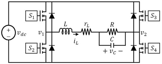
Figure 1. H-bridge inverter circuit.

6.1.1. Sinusoidal Reference Tracking for a Resistive Load

From a control point of view, the objective for such a converter operating in a stand-alone application is to enforce the output voltage $v_C$ to track a sinusoidal reference of the form $y_{ref}=V_{max}sin\left({\omega }_{0}t\right)$. As in the case of PWM inverters, it is considered that the switches of the bridge can be commutated by using bipolar or unipolar strategies [43]. Here, only the case of a bipolar strategy is considered. In this case, the switches of each leg operate complementarily. The high side switch of a leg is off while the low side switch is on, and the high side switch is on when the low side switch is off, leading to a two-level commutation. If we define the control variable u such that $u=1$ when $S_1$ and $S_4$ are on, and $u=-1$ when $S_2$ and $S_3$ are on, the model can be written as follows:

$$\left\{\begin{array}{c}L{\displaystyle \frac{d{i}_L\left(t\right)}{dt}}=-r_L{i}_L\left(t\right)-v_C\left(t\right)+u\left(t\right)V_{in}\hfill \\ C{\displaystyle \frac{d{v}_C\left(t\right)}{dt}}=i_L\left(t\right)-{\displaystyle \frac{v_C}{R}}\left(t\right)\hfill \end{array}\right.$$

Remark that $u\left(t\right)=1$ or $-1$. To have a control $u_1\left(t\right)=0$ or 1, we consider the change in variable $u\left(t\right)=2u_1\left(t\right)-1$, and defining the state vector $x={\left[\begin{array}{cc}{i}_L& v_C\end{array}\right]}^T$, the model of the full bridge can be translated into the canonical form (1).

$$\left\{\begin{array}{c}{\displaystyle \frac{dx\left(t\right)}{dt}}=\underset{A_0}{\underbrace{\left[\begin{array}{cc}-{\displaystyle \frac{r_L}{L}}& -{\displaystyle \frac{1}{L}}\\ {\displaystyle \frac{1}{C}}& -{\displaystyle \frac{1}{RC}}\end{array}\right]}}x\left(t\right)+\left[\underset{B_0}{\underbrace{\left[\begin{array}{c}-{\displaystyle \frac{1}{L}}\\ 0\end{array}\right]}}+\underset{B_{u_1}}{\underbrace{\left[\begin{array}{c}{\displaystyle \frac{2}{L}}\\ 0\end{array}\right]}}{u}_1\left(t\right)\right]V_{in}\hfill \\ y\left(t\right)=\underset{C_0}{\underbrace{\left[\begin{array}{cc}0& 1\end{array}\right]}}x\left(t\right)\hfill \end{array}\right.$$

Matrices associated with the previous model are defined by

$$A_1=A_2=0,B_1=\left[\begin{array}{c}-\frac{1}{L}\\ 0\end{array}\right],B_2=\left[\begin{array}{c}\frac{1}{L}\\ 0\end{array}\right],C_1=C_2=0$$

We consider the full-bridge converter whose parameter values are defined in Table 1.

Table 1. Parameters of the full-bridge inverter.

Parameter	Value	Unit
$V_{\mathrm{in}}$	240	V
$V_{max}$	$120\sqrt{2}$	V
L	390	$\mathsf{\mu }$H
C	$6.2$	$\mathsf{\mu }$F
R	$5.76$	$\mathsf{\Omega }$
$r_L$	$1.5$	$\mathsf{\Omega }$
${\omega }_0$	$2\pi 60$	Rad/s

The reference $y_{ref}$ can be generated from a second-order exosystem whose state space model is

$$\frac{dz\left(t\right)}{dt}=\left[\begin{array}{cc}0& -{\omega }_0\\ {\omega }_0& 0\end{array}\right]z\left(t\right)=\mathsf{\Theta }\left(z\right)\left(t\right),z\left(0\right)=\left[\begin{array}{c}{V}_{max}\\ 0\end{array}\right]$$

with $z\in {\mathbb{R}}^2$. It is possible to express the state reference signal as

$$\begin{array}{ccc}\hfill x_{ref}\left(t\right)& =& \left[\begin{array}{c}{i}_{ref}\left(t\right)\\ v_{ref}\left(t\right)\end{array}\right]=\underset{{\mathsf{\Pi }}_1}{\underbrace{\left[\begin{array}{cc}{\omega }_{0}C& {\displaystyle \frac{1}{R}}\\ 0& 1\end{array}\right]}}z\left(t\right)\hfill \end{array}$$

The control is expressed as

$$arg\left\{\underset{d\in {\mathsf{\Lambda }}_S}{min}{e}^T\left(t\right)P{B}_0\left(x\left(t\right)\right)d\right\} \mathrm{with} B_0\left(x\right)=\left[\begin{array}{cc}{\displaystyle \frac{-V_{in}}{L}}& {\displaystyle \frac{V_{in}}{L}}\\ 0& 0\end{array}\right] \mathrm{and} P=\left[\begin{array}{cc}1.727& 0.033\\ 0.033& 0.033\end{array}\right]$$

Then, an equivalent formulation is

$$\left\{\begin{array}{c}\mathrm{If} e^{T}P{\left[\begin{array}{cc}2V_{in}/L& 0\end{array}\right]}^T>0 \mathrm{then} u_1=0\hfill \\ \mathrm{Otherwise} u_1=1\hfill \end{array}\right.$$

To test the potential and the robustness of the proposed approach, we consider the case in which the input $V_{in}$ is equal to 240 V and changes at $0.02$ s to 320 V, changing after to 230 V at $0.05$ s before returning to 240 V at $0.08$ s. Figure 2 shows the output voltage, inductor current, input voltage and the associated duty cycle. As can be observed, the output tracks the reference and the control is able to compensate the changes in the input voltage $V_{in}$ by accommodating, in an appropriate way, the duty cycle.

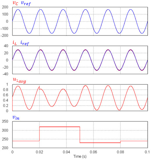
Figure 2. Simulated waveforms of the full-bridge inverter feeding a resistive load.

6.1.2. Sinusoidal Reference Tracking for Nonlinear Loads

Now, the problem is to track a sinusoidal reference for the case in which the loads are nonlinear, illustrating the method proposed in Section 5.2. The output current is supposed to be measured and is considered a measurable perturbation. Now, the basic equations describing the full bridge are given by

$$\left\{\begin{array}{c}L{\displaystyle \frac{d{i}_L\left(t\right)}{dt}}=-r_L{i}_L\left(t\right)-v_C\left(t\right)+u\left(t\right)V_{in}\hfill \\ C{\displaystyle \frac{d{v}_C\left(t\right)}{dt}}=i_L\left(t\right)-i_0\left(t\right)\hfill \end{array}\right.$$

where $w\left(t\right)=i_0\left(t\right)$ is the output current and the state space model writes

$$\left\{\begin{array}{c}{\displaystyle \frac{dx\left(t\right)}{dt}}=\underset{A_0}{\underbrace{\left[\begin{array}{cc}-{\displaystyle \frac{r_L}{L}}& -{\displaystyle \frac{1}{L}}\\ {\displaystyle \frac{1}{C}}& 0\end{array}\right]}}x\left(t\right)+\left[\underset{B_0}{\underbrace{\left[\begin{array}{c}-{\displaystyle \frac{1}{L}}\\ 0\end{array}\right]}}+\underset{B_{u_1}}{\underbrace{\left[\begin{array}{c}{\displaystyle \frac{2}{L}}\\ 0\end{array}\right]}}{u}_1\left(t\right)\right]V_{in}+\underset{E_0}{\underbrace{\left[\begin{array}{c}0\\ -{\displaystyle \frac{1}{C}}\end{array}\right]}}w\left(t\right)\hfill \\ y\left(t\right)=\underset{C_0}{\underbrace{\left[\begin{array}{cc}0& 1\end{array}\right]}}x\left(t\right)\hfill \end{array}\right.$$

The reference is the same $y_{ref}\left(t\right)=V_{max}sin\left({\omega }_{0}t\right).$ From the second state equation, the current reference can be deduced. It is expressed as

$$i_{L_{ref}}\left(t\right)={\omega }_{0}C{V}_{max}cos\left({\omega }_{0}t\right)+i_0\left(t\right)$$

and then the state reference is

$$\begin{array}{ccc}\hfill x_{ref}\left(t\right)& =& \left[\begin{array}{c}{i}_{ref}\left(t\right)\\ v_{ref}\left(t\right)\end{array}\right]=\underset{{\mathsf{\Pi }}_1}{\underbrace{\left[\begin{array}{cc}{\omega }_{0}C& 0\\ 0& 1\end{array}\right]}}z\left(t\right)+\underset{{\mathsf{\Pi }}_p}{\underbrace{\left[\begin{array}{c}1\\ 0\end{array}\right]}}w\left(t\right)\hfill \end{array}$$

The control is expressed as $arg\left\{\underset{d\in {\mathsf{\Lambda }}_S}{min}{e}^T\left(t\right)P[B_0\left(x\left(t\right)\right)+E_0\left(w\left(t\right)\right)]d\right\}$ with

$$B_0\left(x\right)=\left[\begin{array}{cc}{\displaystyle \frac{-V_{in}}{L}}& {\displaystyle \frac{V_{in}}{L}}\\ 0& 0\end{array}\right]x,E_0\left(w\right)=\left[\begin{array}{cc}0& 0\\ -{\displaystyle \frac{1}{C}}& -{\displaystyle \frac{1}{C}}\end{array}\right]w \mathrm{and} P=\left[\begin{array}{cc}1.828& 0.041\\ 0.041& 0.029\end{array}\right]$$

An equivalent formulation is

$$\left\{\begin{array}{c}\mathrm{If} e^{T}P{\left[\begin{array}{cc}2V_{in}/L& 0\end{array}\right]}^T>0 \mathrm{then} u_1=0\hfill \\ \mathrm{Otherwise} u_1=1\hfill \end{array}\right.$$

A first nonlinear load is considered, which corresponds to a Thyristor-Based Rectifier (TBR). The output current in this case has a total harmonic distortion (THD) of approximately 66.34% (see the sinusoidal components used in PSIM simulation in Table 2). Figure 3 represents the output voltage and the inductor current for a numerical experiment in which, at the beginning, $V_{in}$ is equal to 240 V; it then increases to 320 V at $0.02$ s, decreases to 230 V at $0.05$ s and returns to 240 V at $0.08$ s. The control is robust, the output is not affected by the changes in the input voltage and its THD is lower than $0.04\%$. The associated duty cycle, also shown in Figure 3, shows how the control accommodates the duty cycle to tackle the changes in the input voltage and the nonlinearities of the load.

Table 2. Parameters of the TBR-type nonlinear load.

Frequency (Hz)	Amplitude (A)	Phase (Degrees)
60	1.2864	0
180	0.8911	180
300	0.4690	26
420	0.4623	−105
540	0.4623	90
660	0.3484	−69
780	0.2613	143
900	0.2010	−8
1020	0.1273	−147

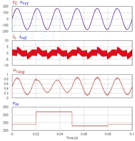
Figure 3. Simulated waveforms of the full-bridge inverter feeding a TBR-type nonlinear load.

A second nonlinear load corresponding to a compact fluorescent lamp (CFL) is also considered. The output current in this case has a THD of approximately $99.84\%$ (see the sinusoidal components used in PSIM simulation in Table 3). The output voltage, inductor current, input voltage and the associated duty cycle are shown in Figure 4. The input voltage $V_{in}$ changes as above. For this load, too, the control is efficient and robust, guaranteeing a THD for the output that is lower than $0.04\%.$

Table 3. Parameters of the CFL-type nonlinear load.

Frequency (Hz)	Amplitude (A)	Phase (Degrees)
60	1.524	−30
180	0.8185	90
300	0.2878	−90
420	0.2728	90
540	0.1636	−90
660	0.1636	90
780	0.1168	−90
900	0.1168	90

Figure 4. Simulated waveforms of the full-bridge inverter feeding a CFL-type nonlinear load.

6.2. Boost Inverter for Stand-Alone Applications

The converter considered in this paragraph is the inverter proposed in [33], whose topology is represented in Figure 5. The parameters used for the simulations are given in Table 4.

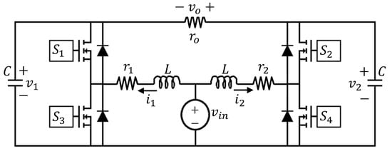
Figure 5. Circuit diagram of the boost inverter.

Table 4. Parameters of the boost inverter.

Parameter	Value	Unit
$V_{in}$	150	V
$V_{max}$	220	V
$V_{dc}$	300	V
$L_1=L_2$	100	$\mathsf{\mu }$H
$C_1=C_2$	2	$\mathsf{\mu }$F
R	100	$\mathsf{\Omega }$
$r_1=r_2$	2	$\mathsf{\Omega }$
${\omega }_0$	$2\pi 50$	rad/s

To model the converter circuit, consider that if $u_1=1$ when $S_1=$ OFF and $S_2=$ ON, $u_1=0$ when $S_1=$ ON and $S_2=$ OFF, and similarly for switches $S_3$ and $S_4$; the elementary electrical equations are given by

$$\left\{\begin{array}{ccc}\hfill L_1{\displaystyle \frac{d{i}_1\left(t\right)}{dt}}& =& -r_1{i}_1\left(t\right)+(u_1\left(t\right)-1)v_{C_1}\left(t\right)+V_{in}\hfill \\ \hfill C_1{\displaystyle \frac{d{v}_{C_1}\left(t\right)}{dt}}& =& (1-u_1\left(t\right))i_1\left(t\right)-{\displaystyle \frac{v_{C_1}\left(t\right)}{R}}+{\displaystyle \frac{v_{C_2}\left(t\right)}{R}}\hfill \\ \hfill L_2{\displaystyle \frac{d{i}_2\left(t\right)}{dt}}& =& -r_2{i}_2\left(t\right)+(u_2\left(t\right)-1)v_{C_2}\left(t\right)+V_{in}\hfill \\ \hfill C_2{\displaystyle \frac{d{v}_{C_2}\left(t\right)}{dt}}& =& (1-u_2\left(t\right))i_2\left(t\right)-{\displaystyle \frac{v_{C_2}\left(t\right)}{R}}+{\displaystyle \frac{v_{C_1}\left(t\right)}{R}}\hfill \end{array}\right.$$

Taking the state vector $x={\left[\begin{array}{cccc}{i}_1\hfill & v_{C_1}\hfill & i_2\hfill & v_{C_2}\hfill \end{array}\right]}^T$, model (1) is expressed as

$$\begin{array}{cc}\hfill \begin{array}{ccc}\hfill {\displaystyle \frac{dx\left(t\right)}{dt}}& =& \left[\underset{A_0}{\underbrace{\left[\begin{array}{cccc}-\frac{r_1}{L_1}& -\frac{1}{L_1}& 0& 0\\ \frac{1}{C_1}& -\frac{1}{R{C}_1}& 0& \frac{1}{R{C}_1}\\ 0& 0& -\frac{r_2}{L_2}& -\frac{1}{L_2}\\ 0& \frac{1}{R{C}_2}& \frac{1}{C_2}& -\frac{1}{R{C}_2}\end{array}\right]}}+u_1\left(t\right)\underset{A_{u_1}}{\underbrace{\left[\begin{array}{cccc}0& \frac{1}{L_1}& 0& 0\\ -\frac{1}{C_1}& 0& 0& 0\\ 0& 0& 0& 0\\ 0& 0& 0& 0\end{array}\right]}}+u_2\left(t\right)\underset{A_{u_2}}{\underbrace{\left[\begin{array}{cccc}0& 0& 0& 0\\ 0& 0& 0& 0\\ 0& 0& 0& \frac{1}{L_2}\\ 0& 0& -\frac{1}{C_2}& 0\end{array}\right]}}\right]x\left(t\right)\hfill \\ & & +\underset{B_0}{\underbrace{\left[\begin{array}{c}\frac{1}{L_1}\\ 0\\ \frac{1}{L_2}\\ 0\end{array}\right]}}{V}_{in}\hfill \\ \hfill y\left(t\right)& =& \underset{C_0}{\underbrace{\left[\begin{array}{cccc}0& 1& 0& -1\end{array}\right]}}x\left(t\right)\hfill \end{array}& \end{array}$$

The idea is to control the inverter while ensuring that the output of each of the two internal boost converters tracks the following reference signals:

$$v_{C_{1_{ref}}}\left(t\right)=V_{dc}+\frac{V_{max}}{2}sin\left({\omega }_{0}t\right)\mathrm{and}{v}_{C_{2ref}}\left(t\right)=V_{dc}-\frac{V_{max}}{2}sin\left({\omega }_{0}t\right)$$

Because the output voltage of a boost converter is greater than the DC voltage source, the following conditions must be satisfied:

$$V_{dc}-\frac{V_{max}}{2}>V_{in}\Rightarrow V_{dc}>V_{in}+\frac{V_{max}}{2}$$

Under these conditions, the reference of the output $y\left(t\right)$ becomes

$$y_{ref}\left(t\right)=v_{C_{1_{ref}}}\left(t\right)-v_{C_{2_{ref}}}\left(t\right)=V_{max}sin\left({\omega }_{0}t\right)$$

The power balance can be obtained from the state space model and is given by

$$L{i}_i\frac{d{i}_i}{dt}+C{v}_{C_i}\frac{d{v}_{C_i}}{dt}=-r_L{i}_i^2+V_{in}{i}_i-\frac{v_{C_i}^2}{R}+\frac{v_{C_1}{v}_{C_2}}{R},i=1,2$$

(21)

As pointed out, determining the inductor current references is quite tedious because such references must satisfy the two previous nonlinear power balance equations, which are difficult to solve analytically. The idea is to approximate the current references using the harmonic balance method [45]. Retaining the first and third harmonics, and because, usually, the circuit is constituted by two boost converters with the same components, the approximation of currents $i_{1_{ref}}\left(t\right)$ and $i_{1_{ref}}\left(t\right)$ is given by

$$\begin{array}{cc}\hfill i_{1_{ref}}\left(t\right)& \simeq I_L+I_{s_1}sin\left({\omega }_{0}t\right)+I_{c_1}cos\left({\omega }_{0}t\right)+I_{s_2}sin\left(2{\omega }_{0}t\right)+I_{c_2}cos\left(2{\omega }_{0}t\right)+I_{s_3}sin\left(3{\omega }_{0}t\right)+I_{c_3}cos\left(3{\omega }_{0}t\right)\hfill \\ \hfill i_{2_{ref}}\left(t\right)& \simeq I_L-I_{s_1}sin\left({\omega }_{0}t\right)+I_{c_1}cos\left({\omega }_{0}t\right)-I_{s_2}sin\left(2{\omega }_{0}t\right)+I_{c_2}cos\left(2{\omega }_{0}t\right)-I_{s_3}sin\left(3{\omega }_{0}t\right)+I_{c_3}cos\left(3{\omega }_{0}t\right)\hfill \end{array}$$

and then the exosystem is defined as

$${\displaystyle \frac{dz\left(t\right)}{dt}}=\mathsf{\Theta }z\left(t\right)=diag\left(\left[\begin{array}{cc}0& -{\omega }_0\\ {\omega }_0& 0\end{array}\right],\left[\begin{array}{cc}0& -2{\omega }_0\\ 2{\omega }_0& 0\end{array}\right],\left[\begin{array}{cc}0& -3{\omega }_0\\ 3{\omega }_0& 0\end{array}\right],0\right)z\left(t\right)$$

with the initial condition

$$z\left(0\right)={\left[\begin{array}{ccccccc}1& 0& 1& 0& 1& 0& 1\end{array}\right]}^T$$

The state reference writes

$$x_{ref}\left(t\right)={\mathsf{\Pi }}_1\left(z\right)\left(t\right)=\left[\begin{array}{ccccccc}{I}_{c_1}& I_{s_1}& I_{c_2}& I_{s_2}& I_{c_3}& I_{s_3}& I_L\\ 0& V_{max}/2& 0& 0& 0& 0& V_{dc}\\ I_{c_1}& -I_{s_1}& I_{c_2}& -I_{s_2}& I_{c_3}& -I_{s_3}& I_L\\ 0& -V_{max}/2& 0& 0& 0& 0& V_{dc}\end{array}\right]z\left(t\right)$$

The amplitudes are obtained by solving the following algebraic system of nonlinear equations:

$$F(I_L,I_{s_1},I_{c_1},I_{s_2},I_{c_2},I_{s_3},I_{c_3})=0$$

where the components of F are given in Appendix A. For the desired output reference, Table 5 gives the values obtained using the MATLAB function fsolve.

Table 5. Amplitudes of reference signals.

${\mathit{I}}_{\mathit{L}}$	${\mathit{I}}_{{\mathit{s}}_1}$	${\mathit{I}}_{{\mathit{c}}_1}$	${\mathit{I}}_{{\mathit{s}}_2}$	${\mathit{I}}_{{\mathit{c}}_2}$	${\mathit{I}}_{{\mathit{s}}_3}$	${\mathit{I}}_{{\mathit{c}}_3}$
$0.9653$	4.5779	$-0.1390$	$0.0197$	$-0.9718$	$-0.0609$	$-0.0020$

The control is defined by

$$(u_1,u_2)=bi{n}_2(j-1)withj=arg\left\{\underset{i=1,2,3,4}{min}{e}^{T}P{A}_{i}x\right\}$$

where $A_1=0,A_2=A_{u_2},A_3=A_{u_1},A_4=A_{u_1}+A_{u_2}$ and P solution of (8) given by

$$P=\left[\begin{array}{cccc}\hfill 2.0933& \hfill 0.0817& \hfill 0.4567& \hfill 0.0183\\ \hfill 0.0817& \hfill 0.0458& \hfill 0.0183& \hfill 0.0092\\ \hfill 0.4567& \hfill 0.0183& \hfill 2.0933& \hfill 0.0817\\ \hfill 0.0183& \hfill 0.0092& \hfill 0.0817& \hfill 0.0458\end{array}\right]$$

Figure 6 depicts the output voltage y and the duty cycles obtained by filtering control $u_1$ and $u_2$ besides the inductor currents $i_1,i_2$ and the capacitor voltages $v_{C_1},v_{C_2}$. We can see that the proposed method leads to satisfactory results for this non-trivial tracking problem.

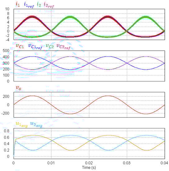
Figure 6. Simulated waveform of the boost inverter feeding a resistive load and using two control actions.

Another means of controlling the inverter is to commute among the configurations associated with $u_1\left(u_2\right)=0\left(1\right)$ and $u_1\left(u_2\right)=1\left(0\right)$. In this case, it is possible to describe this operation mode using only the variable $u_1$, remarking that $u_1\left(u_2\right)=0,(1=1-u_1)$ and $u_1\left(u_2\right)=1(0=1-u_1)$—in other words, replacing $u_2$ with $1-u_1$ in the model above. The model becomes

$$\begin{array}{cc}\hfill \begin{array}{ccc}\hfill {\displaystyle \frac{dx\left(t\right)}{dt}}& =& \left[\underset{A_0}{\underbrace{\left[\begin{array}{cccc}-\frac{r_1}{L_1}& -\frac{1}{L_1}& 0& 0\\ \frac{1}{C_1}& -\frac{1}{R{C}_1}& 0& \frac{1}{R{C}_1}\\ 0& 0& -\frac{r_2}{L_2}& 0\\ 0& \frac{1}{R{C}_2}& 0& -\frac{1}{R{C}_2}\end{array}\right]}}+u_1\left(t\right)\underset{A_{u_1}}{\underbrace{\left[\begin{array}{cccc}0& \frac{1}{L_1}& 0& 0\\ -\frac{1}{C_1}& 0& 0& 0\\ 0& 0& 0& -\frac{1}{L_2}\\ 0& 0& \frac{1}{C_2}& 0\end{array}\right]}}\right]x\left(t\right)+\underset{B_0}{\underbrace{\left[\begin{array}{c}\frac{1}{L_1}\\ 0\\ \frac{1}{L_2}\\ 0\end{array}\right]}}{V}_{in}\hfill \\ \hfill y\left(t\right)& =& \underset{C_0}{\underbrace{\left[\begin{array}{cccc}0& 1& 0& -1\end{array}\right]}}x\left(t\right)\hfill \end{array}& \end{array}$$

(22)

This operation mode is more constrained than the previous one. In particular, determining the state reference is complicated. The difficulty follows from the fact that the power balance Equation (21) must be satisfied by the reference signals, but only one control is now available. In addition, only the reference for the difference $v_{C_1}\left(t\right)-v_{C_2}\left(t\right)$ is available, drastically complicating the determination of the reference signals. This motivates the approximated method introduced in the next section.

7. Approximated State Reference Signal from a Periodic Output Reference Signal

In this section, a method is proposed for determining an approximation of the state reference signal for the case in which the output tracking signal is periodic. In some cases, the computation of the state reference is a significant challenge due the nonlinearities and the switched nature of the power converters. This difficulty was perceived [2] and identified as one of the main difficulties in the control problems of some power converters. This problem is also closely connected to steady state oscillations in nonlinear circuits or mechanical systems, a topic that has attracted the interest of researchers for many years; see, for example, [50,51].

7.1. Approximated State Reference Signal

Recall that the output of the converter is given by

$$y\left(t\right)=C_{0}x\left(t\right)+D_0\left(x\left(t\right)\right)\lambda \left(t\right)=\sum _{i=1}^M{\lambda }_i\left(t\right)(C_0+C_i)x\left(t\right)$$

where the notations are the ones introduced in Section 2. In Section 3, we see that a reference $x_{ref}\left(t\right)$ is admissible if it is a solution of the relaxed converter model recalled below

$$\dot{x}\left(t\right)=A_{0}x\left(t\right)+B_0\left(x\left(t\right)\right)\lambda \left(t\right)=\sum _{i=1}^M{\lambda }_i\left(t\right)(A_0+A_i)x\left(t\right)+\sum _{i=1}^M{\lambda }_i\left(t\right)(B_0+B_i)v_{in}$$

for $\lambda \left(t\right)={\lambda }_{ref}\left(t\right)\in {\mathsf{\Lambda }}_R$. The output reference signal is known because it is the signal that the output must track. We suppose that it is a periodic signal written as

$$y_{ref}\left(t\right)=C_0{x}_{ref}\left(t\right)+D_0\left(x_{ref}\left(t\right)\right){\lambda }_{ref}\left(t\right)$$

(23)

The problem is to deduce the state reference signal from the knowledge of the output reference signal $y_{ref}\left(t\right)$. In general, the maximal frequency contained in the spectrum of the reference $y_{ref}$ is significantly lower than the bandwidth of the converter. Then, the output reference can be seen as a succession of equilibrium points, and, if the output reference $y_{ref}\left(t\right)$ is admissible, there exists a function ${\lambda }_{app}$ such that ${\lambda }_{app}\left(t\right)\in {\mathsf{\Lambda }}_R$ and

$$y_{ref}\left(t\right)=\sum _{i=1}^M{\lambda }_{{app}_i}\left(t\right)(C_0+C_i)x_{app}\left(t\right)$$

(24)

where, for all t, $x_{app}\left(t\right)$ is the solution of the following equation:

$$A_0{x}_{app}\left(t\right)+B_0\left(x_{app}\left(t\right)\right){\lambda }_{app}\left(t\right)=0$$

(25)

Now, supposing that the conditions of Lemma 1 are satisfied, from the previous equation, we can deduce that

$$x_{app}\left(t\right)={\left[\sum _{i=1}^M{\lambda }_{{app}_i}\left(t\right)(A_0+A_i)\right]}^{-1}\left[\sum _{i=1}^M{\lambda }_{{app}_i}\left(t\right)(B_0+B_i)\right]$$

(26)

the invertibility being guaranteed by the conditions of Lemma 1. Replacing in (24), we obtain

$$y_{ref}\left(t\right)=\left[\sum _{i=1}^M{\lambda }_{{app}_i}\left(t\right)(C_0+C_i)\right]{\left[\sum _{i=1}^M{\lambda }_{{app}_i}\left(t\right)(A_0+A_i)\right]}^{-1}\left[\sum _{i=1}^M{\lambda }_{{app}_i}\left(t\right)(B_0+B_i)\right]v_{in}=G\left({\lambda }_{app}\left(t\right)\right)v_{in}$$

(27)

$G\left({\lambda }_{app}\right)$ is simply the gain of the converter for $\lambda ={\lambda }_{app}$. In general, if $y_{ref}\left(t\right)$ is periodic of period T, ${\lambda }_{app}\left(t\right)$ is also periodic of period T. We suppose that this is the case. We can use ${\lambda }_{app}\left(t\right)$ to generate an approximated reference $x_a\left(t\right)$ as the solution of the following differential system:

$$\left\{\begin{array}{ccccc}\hfill {\dot{x}}_a\left(t\right)& =& A_0{x}_a\left(t\right)+B_0\left(x_a\left(t\right)\right){\lambda }_{app}\left(t\right)\hfill & =\hfill & {\displaystyle \sum _{i=1}^M{\lambda }_{{app}_i}\left(t\right)(A_0+A_i)x_a\left(t\right)+\sum _{i=1}^M{\lambda }_{{appr}_i}\left(t\right)(B_0+B_i)v_{in}}\hfill \\ \hfill & & & =\hfill & {\mathcal{A}}_{{\lambda }_{app}}{x}_a\left(t\right)+{\mathcal{B}}_{{\lambda }_{app}}{v}_{in}\hfill \\ \hfill y_a\left(t\right)& =& C_{0}x\left(t\right)+D_0\left(x_a\left(t\right)\right){\lambda }_{app}\left(t\right)\hfill & =\hfill & {\displaystyle \sum _{i=1}^M{\lambda }_{{app}_i}\left(t\right)(C_0+C_i)x_a\left(t\right)}\hfill \\ \hfill & & & =\hfill & {\mathcal{C}}_{{\lambda }_{app}}{x}_a\left(t\right),x_a\left(0\right)=x_{app}\left(0\right)\hfill \end{array}\right.$$

(28)

Summarizing, the approximated state reference signal is determined as follows:

(i)

From the given periodic output reference $y_{ref}\left(t\right)$, and $G\left({\lambda }_{app}\right)v_{in}$, we can compute ${\lambda }_{app}\left(t\right)$;

(ii)

From ${\lambda }_{app}\left(t\right)$ obtained in step i), we can compute $x_a\left(t\right)$, integrating the differential system (28), because ${\lambda }_{app}\left(t\right)\in {\mathsf{\Lambda }}_R$, $x_a\left(t\right)$ is an admissible reference.

The computation can be performed off-line and, because of the periodicity of the signals, it can be restricted to a period and stored in memory. This last aspect is important for implementation issues. When using the approximated reference, it is important to quantify the impact on the tracking error. To evaluate this, note that, combining (25) and (28), we have

$$\left\{\begin{array}{ccc}\hfill {\dot{x}}_a\left(t\right)& =& {\mathcal{A}}_{{\lambda }_{app}}(x_a\left(t\right)-x_{app}\left(t\right))\hfill \\ \hfill \mathsf{\Delta }y\left(t\right)& =& y_a\left(t\right)-y_{ref}\left(t\right)={\mathcal{C}}_{{\lambda }_{app}}(x_a\left(t\right)-x_{app}\left(t\right)),x_a\left(0\right)=x_{app}\left(0\right)\hfill \end{array}\right.$$

(29)

The error $\mathsf{\Delta }y\left(t\right)$ between $y_a\left(t\right)$ and $y_{ref}\left(t\right)$ is the error induced by the approximated state reference signal.

Theorem 4. 

Suppose that the conditions of Lemma 1 are satisfied. Consider an admissible output periodic reference signal of period T, $y_{ref}\left(t\right)$, and consider the associated approximated state reference trajectory $x_a\left(t\right)$ obtained by integrating differential system (28). Then, the following LMI optimization problem

$$\begin{array}{c}{\displaystyle \underset{\mu >0,S=S^T>0}{min}\mu }\\ \left[\begin{array}{ccc}{(A_0+A_i)}^{T}S+S(A_0+A_i)& -S& {(C_0+C_i)}^T\\ -S& -\mu I& 0\\ (C_0+C_i)& 0& -I\end{array}\right]\le 0,i=1,\cdots ,M\end{array}$$

(30)

is feasible and, if $(\overline{\mu },\overline{S})$ denotes its optimal solution, the control

$$\lambda \left(t\right)=arg\left\{\underset{d\in {\mathsf{\Lambda }}_S}{min}{e}^T\left(t\right)\overline{S}\left[A_{0}e\left(t\right)+B_0\left(x\left(t\right)\right)d-B_0\left(x_a\left(t\right)\right){\lambda }_{app}\left(t\right)\right]\right\}=arg\left\{\underset{d\in {\mathsf{\Lambda }}_S}{min}{e}^T\left(t\right)\overline{S}{B}_0\left(x\left(t\right)\right)d\right\}$$

(31)

solves problem 1 for $x_{ref}\left(t\right)$ = $x_a\left(t\right)$. In addition, when $t\to \infty$, it holds that

$${\int }_t^{t+T}{\parallel y_a\left(t\right)-y_{ref}\left(t\right)\parallel }^{2}dt\le \overline{\mu }{\int }_t^{t+T}{∥{\displaystyle \frac{d{x}_{app}\left(t\right)}{dt}}∥}^{2}dt$$

(32)

where $x_{app}\left(t\right)$ satisfies (25).

Proof. 

If the conditions of Lemma 1 are satisfied, there exist positive definite symmetric matrices Q and P such that

$${(A_0+A_i)}^{T}P+P(A_0+A_i)+2Q<0,i=1,\cdots ,M$$

There exists $\alpha >0$ such that $2\alpha Q\ge {(C_0+C_i)}^T(C_0+C_i)$ for $i=1,\cdots ,M$ and we have

$${(A_0+A_i)}^T\alpha P+\alpha P(A_0+A_i)+{(C_0+C_i)}^T(C_0+C_i)\le {(A_0+A_i)}^T\alpha P+\alpha P(A_0+A_i)+2\alpha Q<0$$

Denote $S=\alpha P$. Then, there exists $\mu >0$ sufficiently large such that for $i=1,\cdots ,M$

$${(A_0+A_i)}^{T}S+S(A_0+A_i)+{\mu }^{-1}{S}^2+{(C_0+C_i)}^T(C_0+C_i)<0$$

which, by the Schur complement [49], can be transformed into the inequalities in (30). Then, Problem (30) has a solution denoted $(\overline{\mu },\overline{S})$. From Lemma 1 and the admissibility of approximated reference $x_a\left(t\right)$, the control (31) solves problem 1 for $x_{ref}=x_a$. From Lemma 1, we can also conclude that (28) is an asymptotically stable T-periodic system. It results from Theorem 4.7, p. 101 in [52] or Theorem 1 in [53] that there exists a unique steady-state periodic solution $x_s\left(t\right)$ to (28). This means that when $t\to \infty$,

$$x_a\left(t\right)\to x_s\left(t\right)where{x}_s(t+T)=x_s\left(t\right)$$

Now, consider the function $V(x_a,x_{app})={(x_a-x_{app})}^T\overline{S}(x_a-x_{app})/2$. We have

$$\dot{V}={(x_a-x_{app})}^T\overline{S}\dot{x_a}+{\dot{x_a}}^T\overline{S}(x_a-x_{app})-{(x_a-x_{app})}^T\overline{S}{\dot{x}}_{app}+{\dot{x}}_{app}^T\overline{S}(x_a-x_{app})$$

From (29), ${\dot{x}}_a={\mathcal{A}}_{{\lambda }_{app}}(x_a-x_{app})$; then,

$$\dot{V}={(x_a-x_{app})}^T\left({\mathcal{A}}_{{\lambda }_{app}}^T\overline{S}+\overline{S}{\mathcal{A}}_{{\lambda }_{app}}\right)(x_a-x_{app})-2{(x_a-x_{app})}^T\overline{S}{\dot{x}}_{app}$$

Replace S with $\overline{S}$, $\mu$ by $\overline{\mu }$ in the inequalities (30). Multiplying each of them by ${\lambda }_{{app}_i}\left(t\right)$, summing the obtained terms and taking into account that ${\lambda }_{app}\in {\mathsf{\Lambda }}_R$, we obtain

$$\left[\begin{array}{ccc}{\mathcal{A}}_{{\lambda }_{app}}^T\overline{S}+\overline{S}{\mathcal{A}}_{{\lambda }_{app}}& -\overline{S}& {\mathcal{C}}_{{\lambda }_{app}}^T\\ -\overline{S}& -\overline{\mu }I& 0\\ {\mathcal{C}}_{{\lambda }_{app}}& 0& -I\end{array}\right]\le 0$$

which, by the Schur complement, is also equivalent to

$$\left[\begin{array}{cc}{\mathcal{A}}_{{\lambda }_{app}}^T\overline{S}+\overline{S}{\mathcal{A}}_{{\lambda }_{app}}+{\mathcal{C}}_{{\lambda }_{app}}^T{\mathcal{C}}_{{\lambda }_{app}}& -\overline{S}\\ -\overline{S}& -\overline{\mu }I\end{array}\right]\le 0$$

Multiplying on the left by $\left[{(x_a-x_{app})}^T,{\dot{x}}_{app}^T\right]$ and on the right by its transpose, we have

$${(x_a-x_{app})}^T\left({\mathcal{A}}_{{\lambda }_{app}}^T\overline{S}+\overline{S}{\mathcal{A}}_{{\lambda }_{app}}+{\mathcal{C}}_{{\lambda }_{app}}^T{\mathcal{C}}_{{\lambda }_{app}}\right)(x_a-x_{app})-2{(x_a-x_{app})}^T\overline{S}{\dot{x}}_{app}-\overline{\mu }{\dot{x}}_{app}^T{\dot{x}}_{app}\le 0$$

Then,

$${\displaystyle \frac{dV}{dt}}+{\parallel y_a\left(t\right)-y_{ref}\left(t\right)\parallel }^2-\overline{\mu }{∥{\displaystyle \frac{d{x}_{appr}\left(t\right)}{dt}}∥}^2\le 0$$

which, in turn, by integration with $[t,t+T]$, gives

$$V(x_a(t+T),x_{app}(t+T))-V(x_a\left(t\right),x_{app}\left(t\right))+{\int }_t^{t+T}{\parallel y_a\left(t\right)-y_{ref}\left(t\right)\parallel }^{2}dt-\overline{\mu }{\int }_t^{t+T}{∥{\displaystyle \frac{d{x}_{appr}\left(t\right)}{dt}}∥}^{2}dt\le 0$$

When $t\to \infty$, by the periodicity of $x_a\left(t\right)$ and $x_{app}\left(t\right)$, we have

$${\int }_t^{t+T}{\parallel y_a\left(t\right)-y_{ref}\left(t\right)\parallel }^{2}dt\le \overline{\mu }{\int }_t^{t+T}{∥{\displaystyle \frac{d{x}_{appr}\left(t\right)}{dt}}∥}^{2}dt$$

completing the proof of Theorem 6. □

If $x_{appr}\left(t\right)$ is constant, the right-hand term of (32) is equal to zero and $y_{ref}=x_a\left(t\right)=\mathrm{constant}$. As expected, the error depends on the variations of $x_{app}\left(t\right)$ and $\overline{\mu }$ can be interpreted as a rejection gain when $d{x}_{app}\left(t\right)/dt$ is considered a perturbation signal.

7.2. Numerical Example

Consider the converter depicted in Figure 5, whose parameters are given in Table 4. We consider the case in which the control $u_2$ is equal to $1-u_1$. As explained, it is not easy to determine the state reference signal. The idea is to use the method of the previous paragraph. Recall that the model is given by (22) and that the objective is to impose a reference signal at the output equal to $y_{ref}\left(t\right)=v_{C_{1_{ref}}}\left(t\right)-v_{C_{2_{ref}}}\left(t\right)=V_{max}sin\left({\omega }_{0}t\right)$. From $y_{ref}\left(t\right)$, we must deduce the associated references $v_{C_{1_{ref}}}\left(t\right),$$v_{C_{2_{ref}}}\left(t\right),i_{1_{ref}}\left(t\right)$ and $i_{2_{ref}}\left(t\right)$. Using model (22), after extensive calculation, the expression of the output of the converter (27) is given by

$$y=G\left(\lambda \right)V_{in}={\displaystyle \frac{-\lambda R\left(2\lambda -1\right)\left(\lambda -1\right)}{{\lambda }^{2}R{\left(\lambda -1\right)}^2+r_L\left(2{\lambda }^2-2\lambda +1\right)}}{V}_{in}0<\lambda <1$$

Following the approach proposed in the previous paragraph, ${\lambda }_{app}\left(t\right)$ solution of (25) is obtained solving

$$-\lambda \left(t\right)R{V}_{in}{\displaystyle \frac{\left(2\lambda \left(t\right)-1\right)\left(\lambda \left(t\right)-1\right)}{\lambda {\left(t\right)}^{2}R{\left(\lambda \left(t\right)-1\right)}^2+r_L\left(2\lambda {\left(t\right)}^2-2\lambda \left(t\right)+1\right)}}=y_{ref}\left(t\right)$$

Recall that only the admissible values of $\lambda \left(t\right)$ are real, such that $0<\lambda \left(t\right)<1$. The previous equation can also be written as

$$1+\frac{y_{ref}\left(t\right)}{R{V}_{in}}\frac{\lambda {\left(t\right)}^{2}R{\left(\lambda \left(t\right)-1\right)}^2+r_L\left(2\lambda {\left(t\right)}^2-2\lambda \left(t\right)+1\right)}{\lambda \left(t\right)\left(2\lambda \left(t\right)-1\right)\left(\lambda \left(t\right)-1\right)}=0$$

${\lambda }_{app}\left(t\right)$ is then given by

$${\lambda }_{app}\left(t\right)=\left[\begin{array}{c}1-\lambda \left(t\right)\\ \lambda \left(t\right)\end{array}\right]$$

Invoking the simple root locus building rules, we can easily see that, depending on the sign of $y_{ref}\left(t\right)$, only one root is of interest and varies with $y_{ref}\left(t\right)$ around $1/2$. Then, it is possible to compute the value of $\lambda \left(t\right)$ for a given value of $y_{ref}\left(t\right)$. All the values of $\lambda \left(t\right)$ for a given function $y_{ref}\left(t\right)$ can be determined off-line. Integrating the differential system (28), we deduce the approximated reference $x_a\left(t\right)$ for an output reference given by $y_{ref}\left(t\right)=220sin\left(2\pi 50t\right)$. The resulting waveforms were approximated as Fourier series to implement the simulation in PSIM software as follows:

$$i_{1_{ref}}\simeq 0.99-4.99sin\omega t-0.116cos\omega t+0.068sin2\omega t-1.0145cos2\omega t+0.199sin3\omega t+0.0056cos3\omega t$$

$$i_{2_{ref}}\simeq 0.99+4.99sin\omega t+0.116cos\omega t+0.068sin2\omega t-1.0145cos2\omega t-0.199sin3\omega t-0.0056cos3\omega t$$

$$v_{C_{1_{ref}}}\simeq 318-110sin\omega t-0.903cos\omega t-0.622sin2\omega t-17.387cos2\omega t+0.0015sin3\omega t-0.189cos3\omega t$$

$$v_{C_{2_{ref}}}\simeq 318+110sin\omega t-0.903cos\omega t-0.622sin2\omega t-17.387cos2\omega t-0.0015sin3\omega t+0.189cos3\omega t$$

To determine the control, we solve the optimization problem (30). The solution is given by

$$\overline{S}=\left[\begin{array}{cccc}0.0054& \hfill 0.0000& 0.0000& \hfill 0.0000\\ 0.0000& \hfill 0.0001& 0.0000& \hfill -0.0000\\ 0.0000& \hfill 0.0000& 0.0054& \hfill 0.0000\\ 0.0000& \hfill -0.0000& 0.0000& \hfill 0.0001\end{array}\right],\overline{\mu }=1.39\times {10}^{-7}$$

and the control is given by

$$\mathrm{If} e^T\overline{S}{A}_{2}x>0,u_1=0, \mathrm{otherwise} u_1=1 \mathrm{with} A_2=\left[\begin{array}{cccc}0.& \hfill 1/L& 0& \hfill 0\\ -1/C& \hfill 0& 0& \hfill 0\\ 0& \hfill 0& 0& \hfill -1/L\\ 0& \hfill 0& 1/C& \hfill 0\end{array}\right]$$

Figure 7 shows the currents and the voltages $i_{L_i}$, $v_{C_i}$, $i=1,2$, the output voltage and the duty cycle obtained by filtering the control $u_1$. We can see that the proposed approximated reference trajectories and the resulting control allow us to obtain the expected result. To evaluate more explicitly the error, from the results of Theorem 4, we define the relative error through the indicator

$${\displaystyle \frac{{\displaystyle {\int }_t^{t+T}{\parallel y_a\left(t\right)-y_{ref}\left(t\right)\parallel }^{2}dt}}{{\displaystyle {\int }_t^{t+T}{\parallel y_{ref}\left(t\right)\parallel }^{2}dt}}}\le E(\%)=\overline{\mu }{\displaystyle \frac{{\displaystyle {\int }_t^{t+T}{∥{\displaystyle \frac{d{x}_{app}\left(t\right)}{dt}}∥}^{2}dt}}{{\displaystyle {\int }_t^{t+T}{\parallel y_{ref}\left(t\right)\parallel }^{2}dt}}}=1.39\times {10}^{-7}{\displaystyle \frac{2.63\times {10}^7}{484.00}}=0.76\%$$

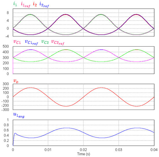
Figure 7. Simulated waveform of the boost inverter feeding a resistive load and using a single control action.

From a practical point of view, the error is acceptable and validates, for the fixed output reference, the proposed approach.

8. Conclusions

This paper proposes a tracking control design method for a large class of converters, extending the results developed in the context of stabilization problems previously published by the authors. Under some assumptions, which can be seen as the expressions of a type of practical feasibility, simple tracking control laws are proposed. The difficulty is related to the determination of the state reference signal from the knowledge of the output reference, this difficulty being the consequence of the nonlinear and switching nature of the power energy converters and from the fact that, in order to apply the proposed techniques, the availability of the state is required. An extension is proposed to take into account possible perturbations. Two alternatives are considered: the case in which perturbations are unknown, and not measurable, and the case in which perturbations are known or can be measured with the help of simple and low-cost sensors. The interest in and potential of the proposed techniques are illustrated in terms of the very popular full-bridge inverter and a fourth-order boost inverter simulated with the PSIM software. In particular, it is discussed in terms of the delicate determination of the reference signals. The method based on the classical harmonic balance method can be used, but for the cases in which this method is not so easy to apply, an alternate technique is proposed. This technique is efficient when the dynamic of the output reference signal is slow compared to the dynamic of the converter.

From the results of simulations, the proposed methods appear very promising and a crucial step is now to apply them to power converter prototypes. This will be carried out in the near future. Several other points could be investigated to improve the method. Among them, the case in which only a measured output is available for control purposes is an important challenge and it can be addressed in terms of the observer-based controllers from which we obtained some partial results. Another interesting problem is to adapt the proposed method to the hybrid control framework in the spirit of the work proposed in [44].

References

- Brockett, R.W.; Wood, J.R. Application of System Theory to Power Processing Problems; Contract NGR 22-007-172; National Aeronautics and Space Administration, NASA Lewis Research Center: Cleveland, OH, USA, 1974. [Google Scholar]
- Sanders, S.R. Nonlinear Control of Switching Power Converters. Ph.D. Thesis, MIT Department EECS, Cambridge, MA, USA, 1989. [Google Scholar]
- Sanders, S.R.; Verghese, G.C. Lyapunov-based control for switched power converters. IEEE Trans. Power Electron. 1992, 7, 17–24. [Google Scholar] [CrossRef] [Green Version]
- Da Silva, W.D. Rethinking the World’s Energy. Cosmos Magazine, 1 April 2012. [Google Scholar]
- Smil, V. A skeptic Looks at alternative energy. IEEE Spectrum 2012, 49, 46–52. [Google Scholar] [CrossRef]
- Armstrong, R.C.; Wolfram, C.; Gross, R.; Lewis, N.S.; Boardman, B.; Ragauskas, A.J.; Ehrhardt-Martinez, K.; Crabtree, G.; Ramana, M.V. The frontiers of energy. Nat. Energy 2016, 1, 15020. [Google Scholar] [CrossRef] [Green Version]
- Kizilyalli, I.C.; Xu, Y.; Carlson, E.; Manser, J.; Cunningham, D.W. Current and Future Directions in Power Electronic Devices and Circuits based on Wide Band-Gap Semiconductors. In Proceedings of the IEEE 5th Workshop on Wide Bandgap Power Devices and Applications (WiPDA), Albuquerque, NM, USA, 30 October–1 November 2017; pp. 417–425. [Google Scholar]
- Cheng, X. Overview of Recent Progress of Semiconductor Power Devices Based on Wide Band Gap Materials. IOP Conf. Ser. Mater. Eng. 2018, 439, 022033. [Google Scholar] [CrossRef]
- Liberzon, D. Switching in Systems and Control; Volume in Series Systems and Control: Foundations and Applications; Birkhauser: Boston, MA, USA, 2003; ISBN 978-0-8176-4297-6. [Google Scholar]
- Goebel, R.; Sanfelice, R.G.; Teel, A.R. Hybrid Dynamical Systems: Modeling, Stability and Robustness; Princeton University Press: Princeton, NJ, USA, 2012. [Google Scholar]
- Sira-Ramirez, H.J.; Silva-Ortigoza, R. Control Design Techniques in Power Electronic Devices; Springer: London, UK, 2006. [Google Scholar]
- Buso, S. Design of a robust voltage controller for a buck-boost converter using μ-synthesis. IEEE Trans. Control Technol 1999, 7, 222–229. [Google Scholar] [CrossRef] [Green Version]
- Olalla, C.; Leyva, R.; Aroudi, A.E.; Queinnec, I. Robust LQR control for PWM converters: An LMI Approach. IEEE Trans. Ind. Electron. 2009, 56, 2548–2558. [Google Scholar] [CrossRef]
- Santos, O.L.; Martinez-Salamero, L.; Garcia, G.; Valderrama-Blavi, H.; Polanco, T.S. Robust Sliding- Mode Control design for a voltage regulated quadratic boost converter. IEEE Trans. Power Electron. 2015, 30, 2313–2327. [Google Scholar] [CrossRef]
- Deaecto, G.; Geromel, J.C.; Garcia, F.; Pomilio, J. Switched affine systems control design with applications to DC-DC converters. IET Control Theory Appl. 2010, 4, 1201–1210. [Google Scholar] [CrossRef]
- Albea, C.; Garcia, G.; Zaccarian, L. Hybrid dynamic modeling and control of switched affine systems: Application to DC-DC converters. In Proceedings of the 54th IEEE Conference on Decision and Control (CDC), Osaka, Japon, 15–18 December 2015. [Google Scholar]
- Hetel, L.; Fridman, E. Robust sampled-data control of switched affine systems. IEEE Trans. Autom. Control 2013, 58, 2922–2928. [Google Scholar] [CrossRef]
- Beneux, G.; Riedinger, P.; Daafouz, J.; Grimaux, L. Adaptive stabilization of switched affine systems with unknown equilibrium points: Application to power converters. Automtatica 2019, 99, 82–91. [Google Scholar] [CrossRef]
- Garcia, G.; Lopez-Santos, O. A unified approach for the control of power electronics converters. Part I Stabilization and Regulation. Appl. Sci. 2021, 11, 631. [Google Scholar] [CrossRef]
- Isidori, A.; Byrnes, C.I. Output regulation of nonlinear systems. IEEE Trans. Autom. Control 1990, 35, 131–140. [Google Scholar] [CrossRef]
- Francis, B.A. The Linear Multivariable Regulator Problem. SIAM J. Control Optim. 1977, 15, 873–878. [Google Scholar] [CrossRef]
- Biemond, J.J.B.; de Wouv, N.V.; Heemeels, W.P.M.H.; Nijmeyer, H. Tracking control for hybrid systems with state-triggered jumps. IEEE Trans. Autom. Control 2013, 58, 876–890. [Google Scholar] [CrossRef] [Green Version]
- Cox, N. Output Regulation for Linear Hybrid Systems with Periodic Jumps. Ph.D. Thesis, University of California, Santa Barbara, CA, USA, 2014. [Google Scholar]
- Carnevale, D.; Galeani, S.; Menini, L.; Sassane, M. Output regulation of linear hybrid systems with unpredictable jumps. In Proceedings of the 19th IFAC World Congress, Cape Town, South Africa, 24–29 August 2014; pp. 1531–1536. [Google Scholar]
- Loukianov, A.G.; Domínguez, J.R.; Castillo-Toledo, B. Robust sliding mode regulation of nonlinear systems. Automatica 2018, 89, 241–246. [Google Scholar] [CrossRef]
- Elmali, H.; Olgac, N. Robust output tracking control of nonlinar MIMO systems via sliding mode technique. Automatica 1992, 28, 145–151. [Google Scholar] [CrossRef]
- Lai, N.O.; Edwards, C.; Spurgeon, S.K. On output tracking using output feedback discrete-time sliding mode controllers. IEEE Trans. Autom. Control 2007, 52, 1975–1981. [Google Scholar] [CrossRef] [Green Version]
- Zheng, B.; Zhong, Y. Robust output regulation for a class of MIMO nonlinear systems with uncertain exo-systems. J. Frankl. Inst. 2013, 350, 1462–1475. [Google Scholar] [CrossRef]
- Govindaswamy, S.; Floquet, T.; Spurgeon, S.K. Discrete-time output feedback sliding mode tracking control for systems with uncertainties. Int. J. Robust Nonlinear Control 2014, 24, 2098–2118. [Google Scholar] [CrossRef]
- Jeong, H.S.; Utkin, V.I. Sliding mode tracking control of systems with unstable zero dynamics. In Variable Structure Systems, Sliding Mode and Nonlinear Control; Young, K.D., Azguner, U., Eds.; Springer: London, UK, 2014; pp. 303–327. [Google Scholar]
- Utkin, V.A.; Utkin, A.V. Problem of tracking in linear systems with parametric uncertainties under unstable zeros. Autom. Remote Control 2014, 75, 1577–1592. [Google Scholar] [CrossRef]
- Bonivento, C.; Marconi, L.; Zanasi, R. Output regulation of nonlinear systems by sliding mode. Automatica 2001, 37, 535–542. [Google Scholar] [CrossRef]
- Cáceres, R.O.; Barbi, I. Boost DC-AC Converter: Analysis, Design, and Experimentation. IEEE Trans. Power Electron. 1999, 14, 134–141. [Google Scholar] [CrossRef]
- Flores-Bahamonde, F.; Valderrama-Blavi, H.; Bosque-Moncusi, J.M.; Garcia, G.; Martinez-Salamero, L. Using the sliding mode approach for analysis and design of the boost inverter. IET Power Electron. 2016, 9, 1625–1634. [Google Scholar] [CrossRef]
- Shtessel, Y.B.; Zinober, A.S.; Shkolnikov, I.A. Sliding mode control, of boost and buck-boost power converters using the dynamic sliding manifold. Int. J. Robust Nonlinear Control 2003, 13, 1285–1298. [Google Scholar] [CrossRef]
- Fossas, E.; Olm, J.M. Galerkin method and approximate tracking in a non minimum phase bilinear system. Discret. Contin. Dyn. Syst. Ser. 2007, 7, 53–76. [Google Scholar] [CrossRef]
- Olm, J.M.; Ros, X. Approximate tracking of periodic references in a class of bilinear systems via stable inversion. Discret. Contin. Dyn. Syst. Ser. 2011, 15, 197–215. [Google Scholar]
- Almawlawe, M.; Mitìc, D.; Antìc, D.; Icìc, Z. An approach to microcontroller-based realization of boost converter with quasi-sliding mode control. J. Circ. Syst. Comp. 2017, 26, 1750106. [Google Scholar] [CrossRef]
- Repecho, V.; Biel, D.; Olm, J.M.; Fossas, E. Robust sliding mode control of a DC/DC boost converter with switching frequency regulation. J. Frank. Inst. 2018, 355, 5367–5383. [Google Scholar] [CrossRef]
- Pandey, S.K.; Patil, S.L.; Phadke, S.B. Regulation of non minimum phase DC-DC converters using integral sliding mode control combined with a disturbance observer. IEEE Trans. Circ. Syst. II Express Briefs 2018, 65, 1649–1653. [Google Scholar]
- Rivera, J.; Ortega-Cisneros, S.; Chavira, F. Sliding mode control output regulation for a boost power converter. Energies 2019, 12, 879. [Google Scholar] [CrossRef] [Green Version]
- Sanchez, C.A.; Lopez-Santos, O.; Zambrano-Prada, D.A.; Gordillo, F.; Garcia, G. Hybrid control scheme for a half- bridge inverter World IFAC Congress. IFAC-PapersOnLine 2017, 50, 9336–9341. [Google Scholar]
- Garcia, G.; Lopez-Santos, O. Unified modeling and control of the full-bridge inverter for stand alone applications. In Proceedings of the Seminario Anual de Automótica, Electrónica Industrial e Instrumentación (SAAEI’19), Córdoba, Spain, 3–5 July 2019. [Google Scholar]
- Albea-Sanchez, C.; Garcia, G.; Hadjeras, S.; Heemels, W.P.M.H.; Zaccarian, L. Practical stabilization of switched affine systems with dwell-time guarantees. IEEE Trans. Autom. Control 2019, 64, 4811–4817. [Google Scholar] [CrossRef] [Green Version]
- Gilmore, R.J.; Steer, M.B. Nonlinear circuit analysis using the method of harmonic balance: A review of the art. Part I. Introductory concepts. Int. J. Microw. Comput.-Aided Eng. 1991, 1, 22–37. [Google Scholar] [CrossRef]
- Ingalls, B.; Sontag, E. An infinite-time relaxation theorem for differential inclusions. Proc. Am. Math. (AMS) 2003, 131, 487–499. [Google Scholar] [CrossRef]
- Whitney, H. Differentiable Manifolds. Ann. Math. Second Ser. 1936, 37, 645–680. [Google Scholar] [CrossRef]
- CortÚs, J. Discontinuous Dynamical Systems. IEEE Control Syst. Mag. 2008, 28, 36–73. [Google Scholar]
- Boyd, S.; Ghaoui, L.E.; Feron, E.; Balakrishnan, V. Linear Matrix Inequalities in Systems and Control; SIAM Studies in Applied Mathematics; SIMA: Philadelphia, PA, USA, 1994; Volume 15. [Google Scholar]
- Hasler, M.; Neirynck, J. Nonlinear Oscillations in Mechanical Engineering; Artech House: Boston, MA, USA, 2005; Volume 454, p. 1986. ISBN 9780890062081. [Google Scholar]
- Fidlin, A. Nonlinear Circuits; Springer Science & Business Media: Berlin/Heidelberg, Germany, 2005; 358p, ISBN 9783540281160. [Google Scholar]
- Coddington, E.A.; Carlson, R. Linear Ordinary Differential Equations; SIAM: Philadelphia, PA, USA, 1997. [Google Scholar]
- Jikuya, I.; Hodaka, I. Time Domain Analysis of Steady State Response in Linear Periodic Systems and Its Application to Switching Converters. IFAC Proc. Vol. 2011, 44, 1307–1312. [Google Scholar] [CrossRef] [Green Version]
Publisher’s Note: MDPI stays neutral with regard to jurisdictional claims in published maps and institutional affiliations. |
© 2021 by the authors. Licensee MDPI, Basel, Switzerland. This article is an open access article distributed under the terms and conditions of the Creative Commons Attribution (CC BY) license (https://creativecommons.org/licenses/by/4.0/).