Use of Linear Viscoelastic Functions to Estimate the Aging Resistance and Internal Structure of Bituminous Binders

Featured Application

The paper provides an analysis of several aging indexes, derived from rheological data, to compare the effect of aging in different formulations of bituminous binders. Using more than one index allows a better evaluation of the complex phenomenon of structural modifications induced by aging.

Abstract

Rheology is the most widely used technique to evaluate the performance and aging of bituminous binders. Since there are many available rheological tests, there is also a wide range of aging indexes and it is not easy to choose the most appropriate one, because a single value may hardly be adequate for different properties or operating conditions. In order to generalize the usefulness of an index, a good starting point is deriving it from a set of data, such as the master curves of linear viscoelastic functions. Then, the problem is the quantification of aging in a single numerical value from continuous curves, covering a wide range of frequencies/temperatures. In this work, a summary of the aging indexes derived from the master curves is reported and discussed. The indexes are applied to a bituminous binder either with or without the addition of an organo-modified layered silicate. The apparent molecular weight distributions and relaxation spectra were also calculated from the master curves and used to characterize the effect of aging on the binder properties and structure. In this way, an interesting parallelism was observed between the SARA fractions and the populations derived from a deconvolution analysis of the apparent molecular weight distributions.

1. Introduction

Aging mainly consists of a hardening process, which comes from the physical–chemical transformations due to the loss of volatiles and partial oxidation of the bitumen component. The related research is focused on different aspects, such as (i) the mechanism and chemistry of the involved reactions; (ii) the effect on performance; and (iii) the strategies to enhance the binder resistance to aging. The first one has been the subject of a huge amount of work and the interested reader may find comprehensive review papers on the topic in the literature, such as those by Petersen [1] and Tauste et al. [2]. With regard to performance, rheology is nowadays the prevalent technique to characterize bituminous binders. It is used to evaluate the performance grade and many other properties, such as the workability or the fatigue and rutting resistance. A comparison of these properties before and after a period of mechanical/oxidative stress, either artificially induced or due to service life, allows quantifying the effects of aging. Due to the high number of available rheological tests, the choice of the aging index is quite subjective and basically any rheological function and/or operating condition can be used to compare the unaged and aged performances [3]. Morian et al., underlined that even if some rheological indexes have good correlation with specific properties, the preferable choice is the development and analysis of full master curves [4]. According to this suggestion, and in order to better clarify the possible choices, we will discuss the available aging indexes that can be directly or indirectly derived from the master curves of the linear viscoelastic functions, such as the phase angle and the magnitude of the complex modulus. Therefore, the analysis starts from the development of viscoelastic master curves, and then continues with the application of the δ-method [5] to obtain the apparent molecular weight distributions (AMWD) and the derivation of the relaxation spectra H($\tilde{\tau }$) [6]. The use of these three different representations, derived from the same experimental data, allows evaluating aging under several points of view. This permits comparing aging indexes with different physical meaning and also to qualitatively evaluate the changes in the colloidal structure of the binder.

Experimental data were derived for a bituminous binder subjected to several degrees of artificial aging both with and without the loading of an organo-modified layered silicate (LS) as anti-ageing additive. Organo-modified LS were first introduced in the field of polymeric materials [7] and the term “organo-modified” indicates that the native clay has been subjected to an ionic exchange reaction, to introduce organic cations into the interlayer spacing. This reduces the hydrophilicity of the clay, thus enhancing its compatibility with bitumens, whose molecules may be driven into the clay galleries. At a high compatibility level, a complete delamination of the clay platelets can be obtained, thus resulting in a dispersion of bi-dimensional platelets with a dimension of a few hundred nanometres and thickness in the order of one nanometre. The high aspect ratio guarantees an extraordinary interfacial interaction between the silicate and bitumen, even at low clay loadings. One of the main consequences related to such interactions is a beneficial effect for the bituminous binders in terms of aging resistance. This has been confirmed by a consistent number of papers and reviews published in the last years [8,9]. Therefore, the use of an organo-modified LS as additive has two advantages in the scope of this work. First, it allows evaluating the sensitivity of the indexes to describe its anti-aging effect with respect to the unmodified binder. Second, the high degree of LS/bitumen interactions may affect the bitumen structure, and this is another aspect that can be evidenced by using the same rheological data and indexes.

2. Materials and Methods

The blends were prepared by using a base bitumen 35/50 penetration grade, referred as B and kindly furnished by Total. The base bitumen derives from a vacuum refinery process and has a Penetration of 38 dmm (UNI EN 1426) and softening point at 56 °C (UNI EN 1427). The organo-modified layered silicate, referred as LS, was supplied by Laviosa. The native clay was a purified montmorillonite, having a dry particle size between 7 and 9 µm, specific weight of 2.2 g/cm³, and a cation exchange capacity, CEC, of 92.5 meq/100 g. The organo modifier was a quaternary ammonium salt.

The LS-B blends were prepared in 350 mL aluminium cans. The cans were partially filled with bitumen and heated to 150 °C and then the LS was added gradually in a few minutes while keeping the system under gentle stirring by using a Silverson L4R. The mixing temperature was selected at 150 °C because it is high enough to guarantee a good fluidity of the binder without risks of degradation of the organic part of the layered silicate. After addition of the clay, the system was maintained under high shear stirring (3600 rpm) for about 30 min. Wide angle X-ray scattering showed that the LS-B nanocomposites structure was predominantly intercalated.

2.1. Artificial Aging

Artificial aging consists of heating the binder in the presence of oxidative agents and this can be done with different setups, often approved and described in standards as ASTM or UNI-EN [10]. In our study, the binders were long-term aged by using the Pressure Aging Vessel (PAV). The conventional Rolling Thin Film Oven (RTFO) followed by 20 h of PAV was substituted by a 25 h PAV, as suggested by Lesueur [11]. Then, additional PAV exposures until 40, 65, and 90 h were conducted in analogue operating conditions (100 °C and air pressure of 2.1 ± 0.1 MPa). In what follows the samples are indicated as B or LS-B followed by hours of PAV aging. As an example, LS-B25 indicates the LS-B blend after 25 h of PAV.

2.2. Rheology

Frequency sweep tests were conducted using a Malvern Kinexus PRO Dynamic Shear Rheometer (DSR). Data were collected under isothermal condition within the linear viscoelastic region. The investigated temperature range varied from −10 to 70 °C, being the lower and higher temperature based on the binder aging (the higher the aging level, the higher the temperatures). The loading frequency varied according to a logarithmic ramping scale from 0.1 to 10 Hz (0.63 to 6.3 rad/s). Depending on the aging degree and temperature, parallel plates of 8 and 25 mm were used. While shifting from one geometry to another, data collected at two overlapping temperatures with both geometries were compared to evaluate their reliability. The temperature range was selected to gather the broader range of phase-angle values. The isotherms were then used to build master curves by applying the time–temperature superposition principle (TTSP), which was valid for both binders at all aging levels [6]. The horizontal shift factors (a_T) were used to build the phase-angle master curves. Then the same shifting was applied to the isotherms of the complex modulus. In some cases, like for many polymeric materials, this is enough to obtain continuous and smooth curves for all dynamic functions. However, for bituminous materials, it is often necessary to add a vertical shifting (which does not affect the phase-angle curves), which is related to the variation in density with temperature. It is worth underlining that at the end of the procedure, for each binder, the final horizontal and vertical shift are the same irrespective of the dynamic function.

The reference temperature for all master curves was fixed at 0 °C. The master curves of the phase-angle and complex modulus were used to calculate the apparent molecular weight distributions and the relaxation spectra respectively. 0 °C was chosen because this is the reference temperature for Equation (2), described in the following subsection and used in the application of the δ-method.

2.3. Apparent Molecular Weight Distributions

For several years rheologists have been trying to link the molecular weight distributions (MWD) with the rheological data. The first papers were dedicated to polymers [12,13] and then the same approach was extended to bituminous binders [14,15]. One of the suggested procedures is the so-called δ-method, recently developed by Themeli and co-workers [5]. The method is described in detail in the original paper and is based on the idea that relaxation frequencies of the molecules are directly correlated with their molecular weight. In inhomogeneous systems, such as polymers or bituminous binders, this corresponds to a distribution of the relaxation frequencies (ω) that is directly correlated with the phase-angle (δ) master curve. At a given frequency, the higher the number of molecules with a lower relaxation frequency, the higher the phase angle. This leads to the assumption that the cumulative molecular weight distribution (CMWD) is proportional to δ(ω). In other words, the master curve of the phase angle is directly converted into CMWD by applying the simple normalization:

$$CMWD=\frac{1}{90}\delta \left(MW\right)$$

(1)

where δ (MW) is the phase angle expressed as a function of the molecular weight.

Therefore, all that is needed to convert the phase-angle master curve into an MWD is a correlation between ω and the molecular weight (MW). The chosen correlation is the one developed by Zanzotto et al. [14] through vapour pressure osmometry.

log (𝑀𝑊) = 2.88 − 0.06768log (𝜔_c)

(2)

where 𝜔_c is the crossover frequency (at which the phase angle is equal to 45°) at 0 °C. The last step to convert the cumulative distribution into the more commonly used weight fraction (w) is the differentiation of the CMWD with respect to log(MW):

$$w\left(MW\right)=\frac{d\left(CMWD\right)}{d\left(\log \left(MW\right)\right)}$$

(3)

It is worth underlining that a complete MWD may be obtained only if a master curve covering the whole range of phase angles (from 0 to 90°) is available. Moreover, the smoothness of the curve is important for the derivation of the MWD by differentiating the CMWD [16]. For these two reasons, it may be useful to fit the experimental data with a rheological model. This allows both extrapolating the curve where experimental data are missing (phase-angle values close to 0°) and an easier data manipulation. Among the long list of available models (see the review by Yusoff et al. [17]), we chose 2S2P1D [18,19,20,21], consisting of a combination of two springs, two parabolic elements, and one dashpot (Equation (4), Figure 1).

$$G^{*}=G_o+\frac{\left(\left|G_{\infty }\right|-\left|G_o\right|\right)}{1+\alpha {\left(i\omega \tau \right)}^{-k}+{\left(i\omega \tau \right)}^{-h}+{\left(i\omega \beta \tau \right)}^{-1}}$$

(4)

where G* is the complex modulus; |G_∞| and |G₀| are the magnitudes of the complex modulus at angular frequency ω approaching infinite and zero, respectively; α, β, τ, k, and h are the model parameters; and i is the imaginary unit. It is worth nothing that in the literature, |G_∞| is often indicated as |G_g| and referred as the “Glassy modulus”. The expression for the phase angle can be derived from Equation (4) by applying the properties of complex numbers as follows. G* can be expressed in terms of real and imaginary parts:

$$G^{*}=G^{\prime }+i{G}^{″}$$

(5)

If we introduce the complex number A* defined as

$$A^{*}=1+\alpha {\left(i\omega \tau \right)}^{-k}+{\left(i\omega \tau \right)}^{-h}+{\left(i\omega \beta \tau \right)}^{-1}=A^{\prime }-i{A}^{″}$$

(6)

where A′ and A″ are the real and imaginary parts of A*; then we obtain

$$A^{\prime }=1+\frac{\alpha cos\left(k\pi /2\right)}{{\left(\omega \tau \right)}^k}+\frac{cos\left(h\pi /2\right)}{{\left(\omega \tau \right)}^h}$$

(7)

$$A^{″}=1+\frac{\alpha sin\left(k\pi /2\right)}{{\left(\omega \tau \right)}^k}+\frac{sin\left(h\pi /2\right)}{{\left(\omega \tau \right)}^h}+\frac{1}{\omega \beta \tau }$$

(8)

Combining Equations (5)–(8) gives

$$G^{\prime }=\left|G_0\right|+\frac{\left(\left|G_{\infty }\right|-\left|G_o\right|\right)A^{\prime }}{{\left|A^{*}\right|}^2}$$

(9)

$$G^{″}=\frac{\left(\left|G_{\infty }\right|-\left|G_o\right|\right)A^{″}}{{\left|A^{*}\right|}^2}$$

(10)

where |A*| is the magnitude of A*. Finally, the phase angle is obtained as

$$\delta =arctan\left(\frac{G^{″}}{G^{\prime }}\right)$$

(11)

The above-listed model parameters were calculated by minimizing the following error function (E):

$$E\left(\lceil G_0\rceil ,\lceil G_{\infty }\rceil ,\alpha ,\beta , \tau ,k,h\right)={\displaystyle \sum }_{j=1}^N{\left(\frac{\left[{\delta }_{j,exp}\left(\omega \right)-{\delta }_{j,2S2P1D}\left(\omega \right)\right]}{{\delta }_{j,exp}\left(\omega \right)}\right)}^2$$

(12)

where N is the total number of experimental data in the phase-angle master curve; δ_j,exp (ω) are the experimental data of the phase angle; and δ_j,2S2P1D (ω) the corresponding values calculated with the model. Microsoft Excel Solver^® was used for the computation of Equation (12).

Distributions derived from rheological data are referred to as “apparent” molecular weight distributions, to underline the indirect determination from bulk measurements. In bulk, the mobility of the molecules depends on their dimension and on their interactions with the surrounding molecules. Therefore, the relaxation frequencies of the molecules depend on both their molecular weight (dimension) and polarity (interactions). In other words, the AMWD detects the appearance of new functional groups, due to oxidation, even if they do not alter significantly the molecular weight of the molecules, because they alter the interactions with other molecules. While evaluating the effects of aging, this is an advantage with respect to a technique such as gel permeation chromatography (GPC) or osmometry, which imply the use of a solvent. Indeed, GPC detects the distribution in a diluted media, where bitumen molecules are supposedly isolated one from each other and their interactions with other bitumen molecules are substituted by interactions with solvent molecules. For this reason, GPC gives a picture of the real molecular weight distribution, which is less affected by oxidative aging that has the abovementioned scarce influence on the molecular weight of the bitumen molecules. Both approaches, in bulk or in dilute conditions, have advantages and disadvantages as well as experimental uncertainties [22,23]. Therefore, they do not give a reliable absolute value of the molecular weight, but they give a useful tool to compare distributions of materials with similar origin and chemical composition. Since an absolute value of the molecular weight remains affected by numerous uncertainties, the approach of using the techniques based on solvents to calibrate those based on bulk measurements appears justified, thus obtaining comparable values of the distributions [5,14,24].

2.4. Relaxation Spectrum

The relaxation spectrum H($\tilde{\tau }$) gives another important picture of the material behaviour, especially when dealing with aging. To help visualise the physical meaning of the relaxation spectrum, the reader may refer to the well-known generalised Maxwell model, composed of a virtually infinite number of springs and dashpots connected in parallel [6,24]. Each element is characterized by its elastic constant and relaxation time. At a fixed temperature, the rheological behaviour of any material can be described by this model when using a large-enough number of elements. Then, the discrete relaxation spectrum is given by the plot of the elastic constants as a function of the corresponding relaxation times. If the number of elements goes to infinite, the result is a continuous spectrum. The interested reader may find an accurate mathematical description of this rheological function in Reference [6].

Oxidative aging affects the relaxation spectra for the same reasons it affects the AMWD. This is why H($\tilde{\tau }$) can be directly linked to the AMWD and used as an aging indicator. A direct measurement of H($\tilde{\tau }$) is not easy from an experimental point of view and the preferred way is usually an approximate calculation from other rheological data. Among the long list of available procedures [25,26,27], we used the following approximation, easily applicable to the abovementioned 2S2P1D model:

$$H\left(\tilde{\tau }\right)=\pm \frac{1}{\pi }Im\left[G^{*}\left(\frac{1}{\tilde{\tau }}{e}^{\pm i\pi }\right)\right]$$

(13)

where Im indicates the imaginary part of the quantity written in square brackets, which is the complex modulus obtained by replacing iω by $\tilde{\tau }$⁻¹exp(±iπ) in Equation (4). In other words, the relaxation spectrum can be determined from any analytic expression of G*(iω) by substituting iω with 1/$\tilde{\tau }$ exp (±iπ) and then dividing the imaginary part of G* by π. A detailed description of how Equation (13) can be obtained by applying the theory of integral transforms to correlate the relaxation spectrum and a linear viscoelastic functions as G* is reported in the paper by Liu et al. [28].

2.5. High-Performance Thin-Layer Chromatography (HPTLC)

Due to bitumen’s extreme molecular complexity, chromatography techniques [29] have been frequently used over the decades to determine its constitution. Based on its polarity, bitumen can be separated into four generic fractions called SARA (saturates, aromatics, resins, and asphaltenes) by using chromatography devices such as Iatroscan Thin-Layer Chromatography (TLC) coupled with a flame ionization detector (FID) or automated High-Performance Layer Chromatography (HPLC) SAR-AD^®. To perform this separation, a specific method has been used by TOTAL based on an HPTLC apparatus (High-Performance Thin Layer Chromatography). Analysis was performed on 10 cm × 20 cm pre-coated (silica gel 60F254; Merck, New York, NY, USA) HPTLC plates. The deposit bandwidth was 4 mm × 0.2 mm. A combination of solvents was used to ensure the migration and separation of each fraction (THF, DCM and/or heptane). The plates were subjected to scanning at 280 nm for aromatics, resins, and asphaltene fractions and 365 nm (with induced fluorescence by berberine) for the saturates fraction by means of a TLC scanner 3 (Camag) in absorbance/reflection mode and subsequently processed by CATS software (CAMAG).2.6 [30].

The organization of the research is summarized in Scheme 1, which gives a picture of how the paper is organized from the experimental point of view.

3. Results and Discussion

3.1. Master Curves

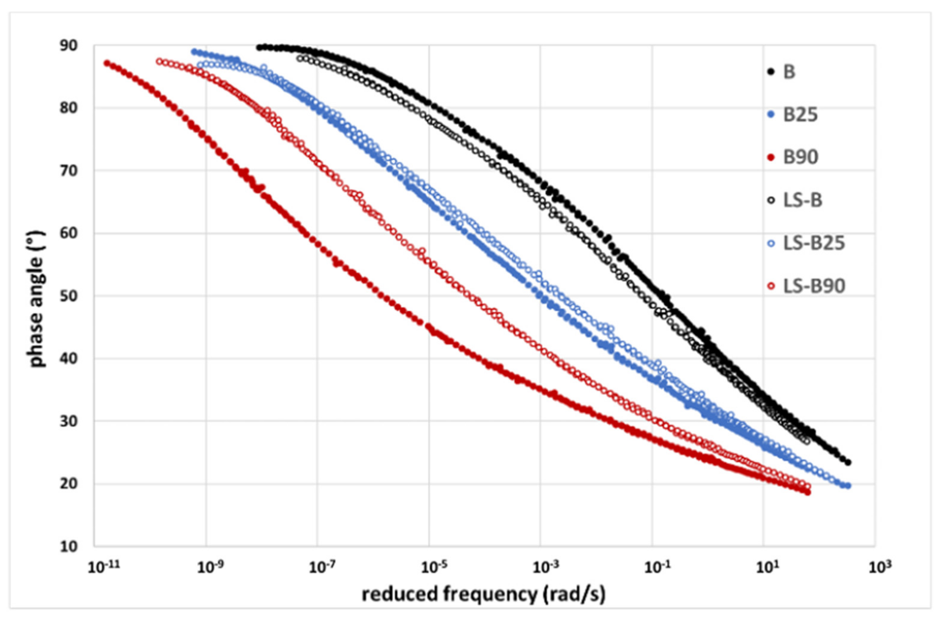
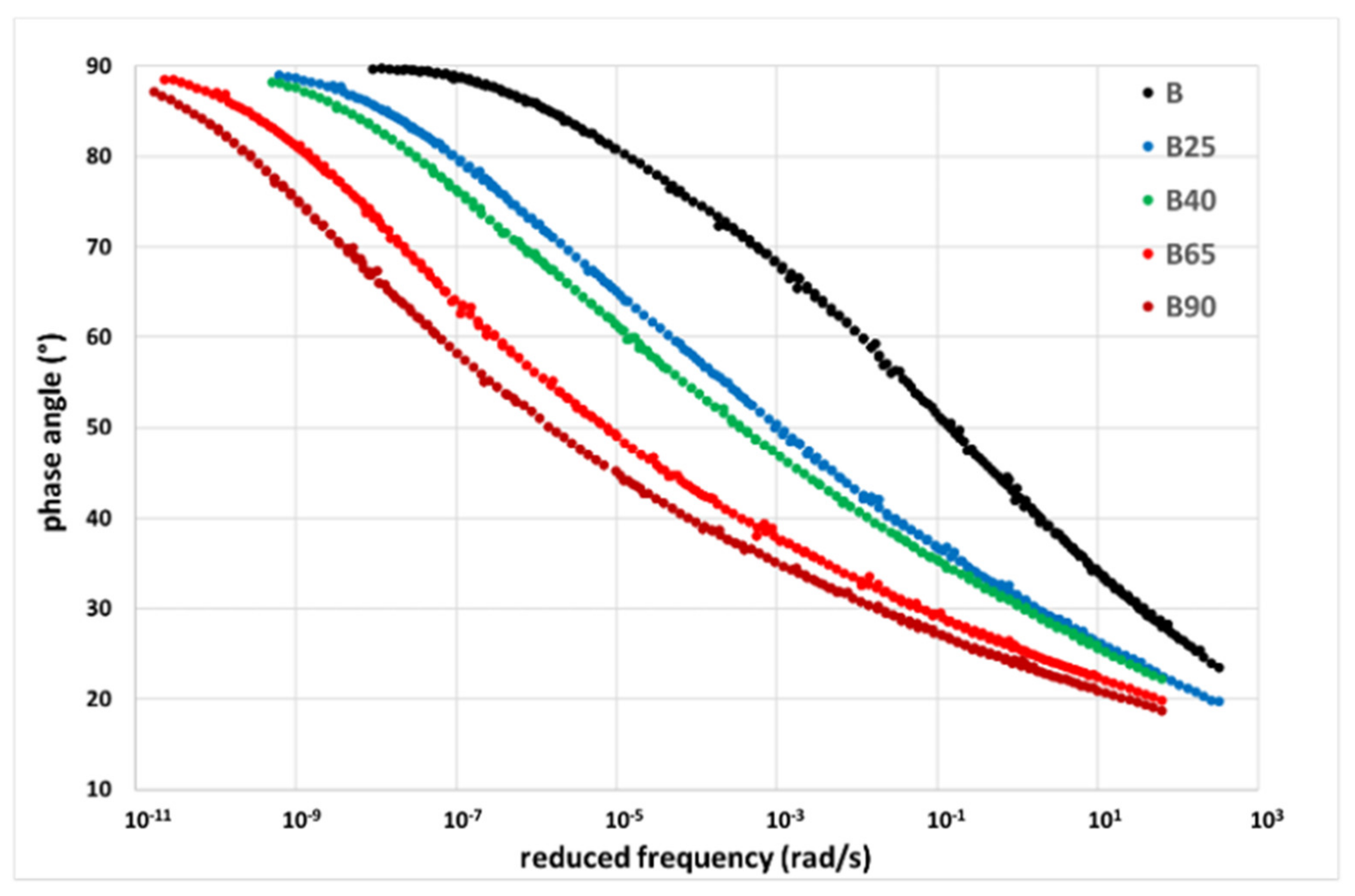
Figure 2 shows the phase-angle master curves derived for the base binder by application of the TTSP. The master curves at all levels of aging have the typical behaviour of bitumen, which in a relatively short frequency range changes from a low-viscosity Newtonian liquid to a glassy, brittle solid. In the intermediate frequency range, bitumen has viscoelastic properties directly related to its colloidal structure, determined by the composition and relative amount of maltenes and asphaltenes [3,4]. It is in this range that even small variations in the composition caused by the oxidative aging may have a significant effect on the rheological behaviour. This is clearly visible by observing the changes induced by multiple PAV cycles. From a qualitative point of view, the increase in bitumen stiffness is reflected by a reduction in the values of the phase angle (at a fixed reduced frequency) that determines a shift of the whole curve toward lower reduced frequencies.

A qualitatively similar behaviour can be observed for the master curves of the LS-B binders and it is interesting to compare the master curves with and without clay, reported in Figure 3 for some of the aging levels. Undoubtedly, LS has a remarkable impact on the aging behaviour. The unaged binders have similar values of the phase angle, the LS-B binder being a little bit stiffer due to the presence of the solid modifier. The relative position of the curves reverses after 25 h of PAV aging and the distance between the curves increases significantly at very high levels of aging. Considering the logarithmic scale of the x-axis, it is clear that for intermediate values of δ, the reduced frequency may vary even by one order of magnitude while comparing the two binders. This is the first indication of an anti-aging effect of the clay.

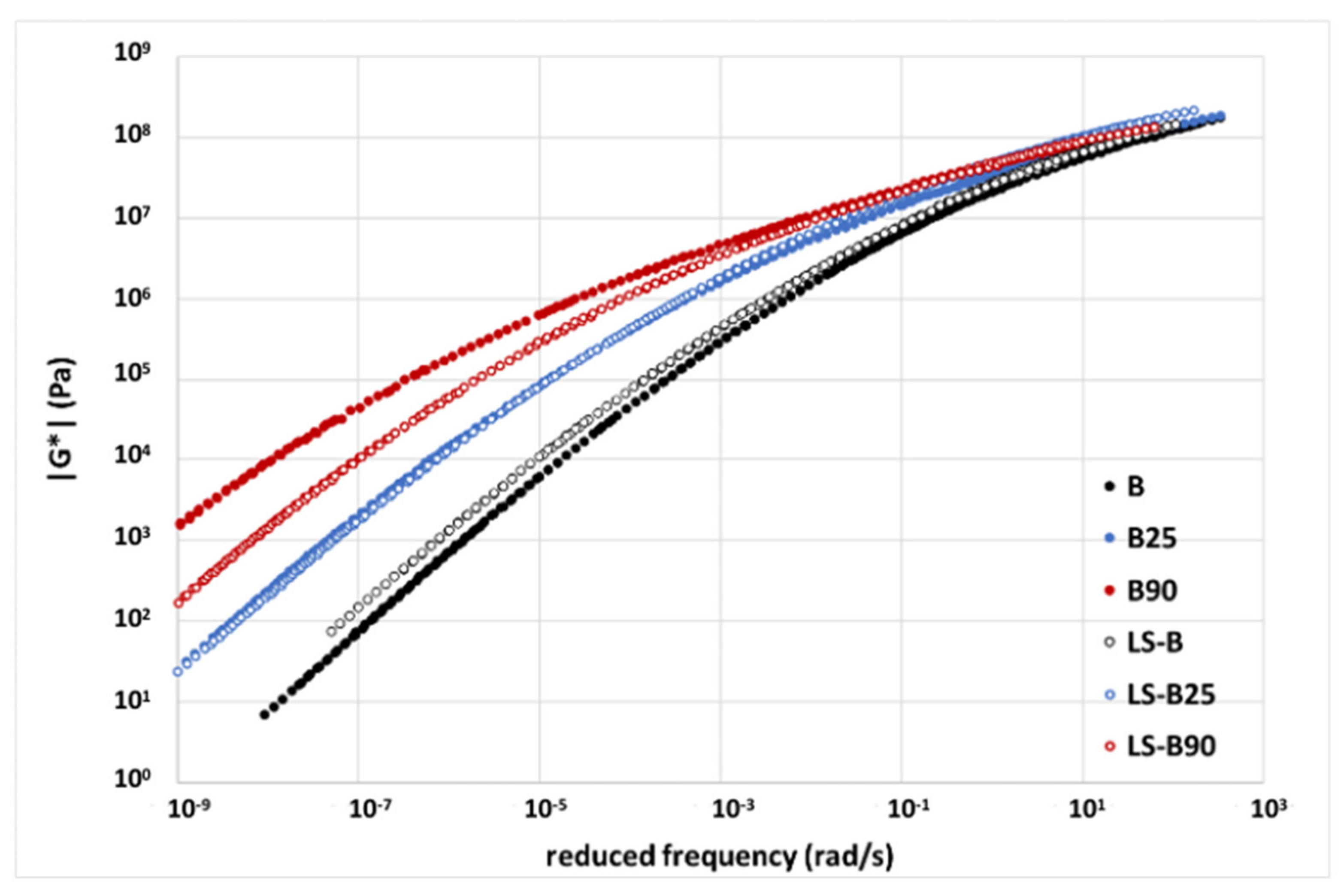
The master curves of the magnitude of complex modulus (Figure 4) confirm the described trend. The |G*| value increases with aging and its variation is much higher without clay. Before aging, the curve of B has a lower magnitude of the modulus with respect to LS-B; after 25 h of PAV the curves are almost superposed, while an inversion is observed after further PAV treatments.

A quantitative evaluation of the aging can be performed in several ways, depending on the used aging index. Usually, the aging indexes are calculated as the ratio between a property before and after aging. This property can be chosen among the classical ones for bituminous binders (e.g., softening point, Brookfield viscosity, or penetration) or can be related to the chemical composition by evaluating the degree of oxidation (i.e., C=O groups quantified by infra-red spectra) [31]. Otherwise, it can derive from rheological data and this opens the debated question about the most representative indexes [3,4]. One reason why the choice is not easy, is that rheological data usually derive from frequency, temperature, stress, or strain sweeps, and thus cover a wide range of operating conditions. 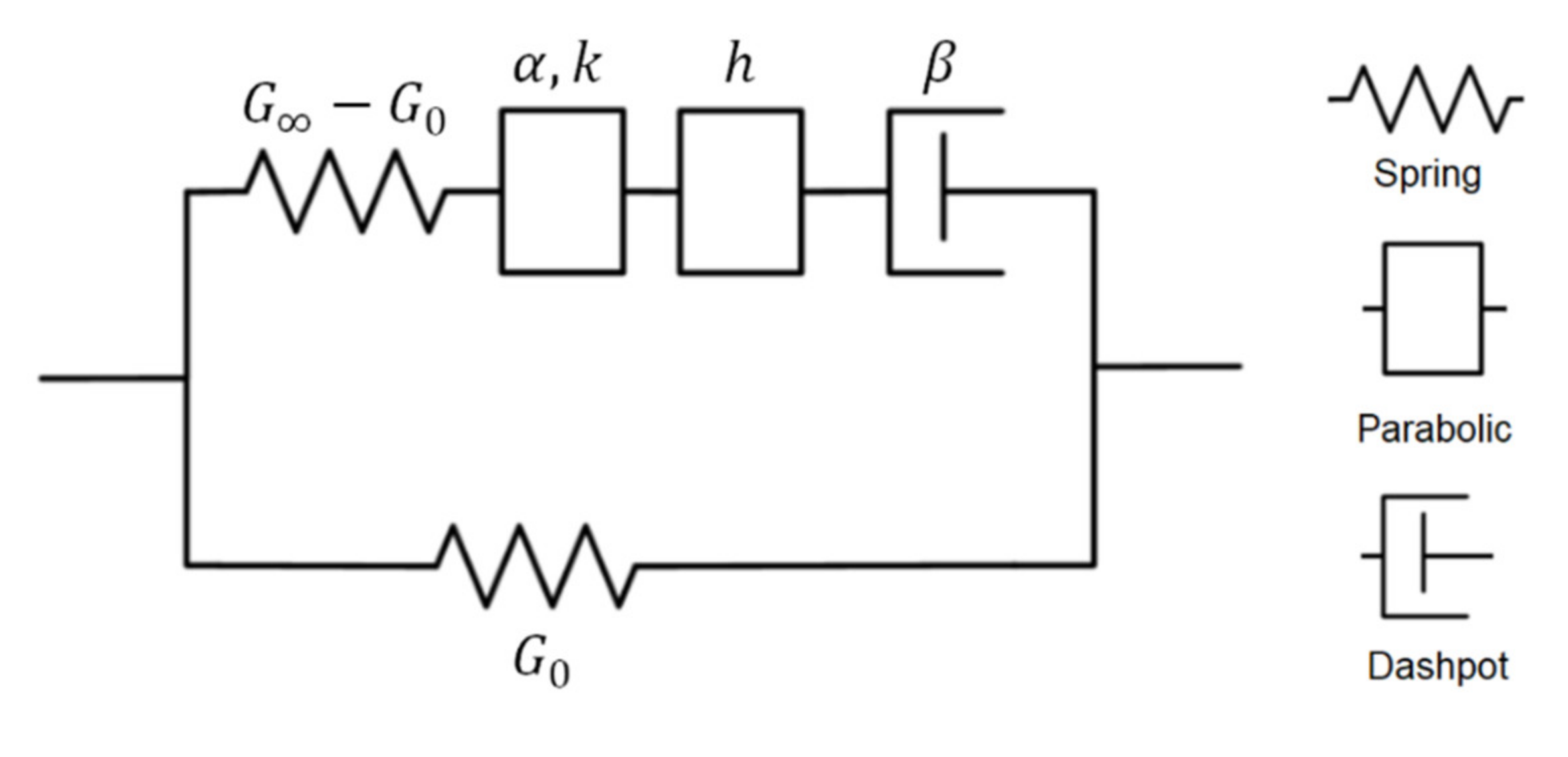Evaluating the aging index on a single point of a long curve, such as the master curves of Figure 2, Figure 3 and Figure 4, may not be fully representative. In contrast, deriving an “aging master curve” by considering all experimental data may be as much useless or dispersive and difficult to interpret. A possible solution is the use of parameters that somehow describe the curve shape, such as those derived from the Christensen–Andersen model [32]. This model describes the complex modulus of bituminous binders and asphalt mixtures by the following expression:

$$\left|G^{*}\left(\omega \right)\right|=\left|G_{\infty }\right|{\left[1+{\left(\frac{{\omega }_c}{\omega }\right)}^{\frac{log2}{R}}\right]}^{\frac{-R}{log2}}$$

(14)

which contains only three parameters: |G_∞|, the crossover frequency ω_c, and the so-called rheological index R. The latter is a “shape parameter” and represents the difference between the logarithmic values of |G_∞| and |G_c| (crossover modulus = complex modulus at the crossover frequency). Generally, the master curve of |G*| becomes flatter as a consequence of aging and thus the increase in R can be used to estimate the level of aging. Ling et al., suggested a power law for the dependence of R from the aging time [33]. Moreover, the above-described shift to the left of the curve can be identified through the crossover frequency and thus two out of the three parameters of the CA model are directly connected with aging. The third parameter is the glassy modulus and often is not directly available since it may require recording data at low temperatures by means of torsion bars. In some cases, this value is simply treated as a fitting parameter and thus extrapolated from the intermediate temperatures. Alternatively, a constant value (1 GPa) is arbitrarily assumed as valid irrespective of the aging degree and in this case the CA model has only two parameters, with R = R(|G_c|) [34]. Both solutions are questionable, but probably the assumption of a fixed glassy modulus has a better chance to fit with reality. It is important to underline that thanks to their physical meaning, the parameters can be directly extrapolated from the |G^*| master curves without applying the CA model to fit the curve and this is what we did. In other words, here Equation (14) is reported only to introduce the physical meaning of these parameters and not used to fit the master curves, and the values of R and ω_c were taken directly from the experimental data reported in Figure 4. The numerical values for these parameters are reported in

Table 1. Values of R, ω_c, and log(|G_c|) from the experimental master curves and the corresponding aging indexes defined in Equation (15).

	B					LS-B
PAV	R	ωc (rad/s)	AIR	AIω	Log (|Gc|)	R	ωc (rad/s)	AIR	AIω	Log (|Gc|)
0	1.80	5.36 · 10−1	0	0	7.2	1.86	2.57 · 10−1	0	0	7.14
25	2.42	4.94 · 10−3	0.35	7.53	6.58	2.16	1.19 · 10−2	0.16	2.26	6.84
40	2.56	2.19 · 10−3	0.42	8.83	6.44	2.44	5.51 · 10−3	0.31	2.83	6.56
65	2.97	5.74 · 10−5	0.66	14.7	6.03	2.85	4.28 · 10−4	0.54	4.71	6.15
90	3.20	9.87 · 10−6	0.78	17.5	5.8	2.72	3.02 · 10−4	0.47	4.97	6.28

, together with the corresponding aging indexes AI_R and AI_ω defined as follows:

$$A{I}_R=\frac{\left(R_a-R_u\right)}{R_u}\hspace{1em}\hspace{1em}\hspace{1em}A{I}_{\omega }=\frac{\left(\log {\omega }_{c,a}-\log {\omega }_{c,u}\right)}{\log {\omega }_{c,u}}$$

(15)

where the subscript a and u indicate aged and unaged, respectively, and ω_c is expressed in rad/s. For the calculation of R in Table 1, |G_∞| was assumed equal to 1 GPa. The variation in R indicates that the crossover moduli varies 1.4 orders of magnitude without clay and less than one order of magnitude with the clay. Even more pronounced is the shift of the crossover frequency, which varies of about five orders of magnitude for B and only three with clay (LS-B binder). The aging indexes clearly reflect these differences, AI_ω being the one that has the higher sensitivity in this case. Moreover, it is interesting to observe that between 65 and 90 h of PAV the properties of LS-B remain almost constant, while those of B are still subjected to significant changes.

As already underlined, even if useful and widely accepted, the disadvantage of R is its dependence on |G_∞|, which can be uncertain. Therefore, as an alternative with a higher chance of being included in the experimental master curve, the evolution of the crossover modulus |G_c| can be considered. Indeed, due to the assumption of |G_∞| being constant and equal to 10⁹ Pa, the logarithm of the crossover moduli is given by 9-R, also reported in Table 1. Oldham et al. [35] underline that log |G_c| can be linked to the dispersion index (DI, ratio between the weight and number average molecular weights), which, in turn, has a direct link with the material composition and thus with aging. The crossover modulus decreases and DI increases due to the chemical oxidation that favours the aggregations between molecules. Analogously, Farrar et al. [34] correlate the inverse of log |G_c| with the total oxygen content. Of course, the trend is the same observed for R and thus we can read these data as an indication of a lower DI and lower oxygen uptake while dealing with LS-modified binders. This point will be further discussed in Section 3.3.

Another possible way to quantitatively correlate the master curves and aging is through the variation of the shift factors used in the TTSP. Although there are many possibilities in the analytical description of the horizontal shift factors [36], in bitumen practice the most widely used ones are the William–Landel–Ferry (WLF) equation,

$$\log a_T\left(T,T_r\right)=\frac{-C_1\left(T-T_r\right)}{C_2+\left(T-T_r\right)},$$

(16)

and Arrhenius equation,

$$\log a_T=\frac{0.4347E_a}{R}\left(\frac{1}{T}-\frac{1}{T_r}\right),$$

(17)

where C₁ and C₂ are the WLF parameters, T_r is the reference temperature (K), R is the ideal gas constant, and E_a is the activation energy for flow. The variation of the shift factors, or alternatively of the parameters of Equations (16) and (17), can be monitored as a function of aging. As an example, Morian et al., showed that variations of parameters C₁ and C₂ with aging correlates with the growth of carbonyl groups [4]. Analogously, the same parameters showed a relationship with the asphaltenes content [37] and thus with aging, C₁ being the most reliable indicator [38]. In our case, the shift factors showed a better correlation with Equation (17) and the obtained values of the activation energies are reported in

Table 2. Activation energies (kJ/mol).

	B		LS-B
PAV	Ea (kJ/mol)	AI (Ea,a/Ea,u)	Ea (kJ/mol)	AI (Ea,a/Ea,u)
0	165	1.00	162	1.00
25	184	1.12	182	1.12
40	190	1.15	185	1.14
65	198	1.20	188	1.16
90	197	1.19	185	1.14

together with the corresponding aging index, defined as the ratio between the activation energies in the aged (E_a,a) and unaged (E_a,u) samples.

The trend in the aging indexes confirms the previous findings, but the numerical values seems to be slightly sensitive to aging and no significant variation in the activation energies is observed for the longest aging.

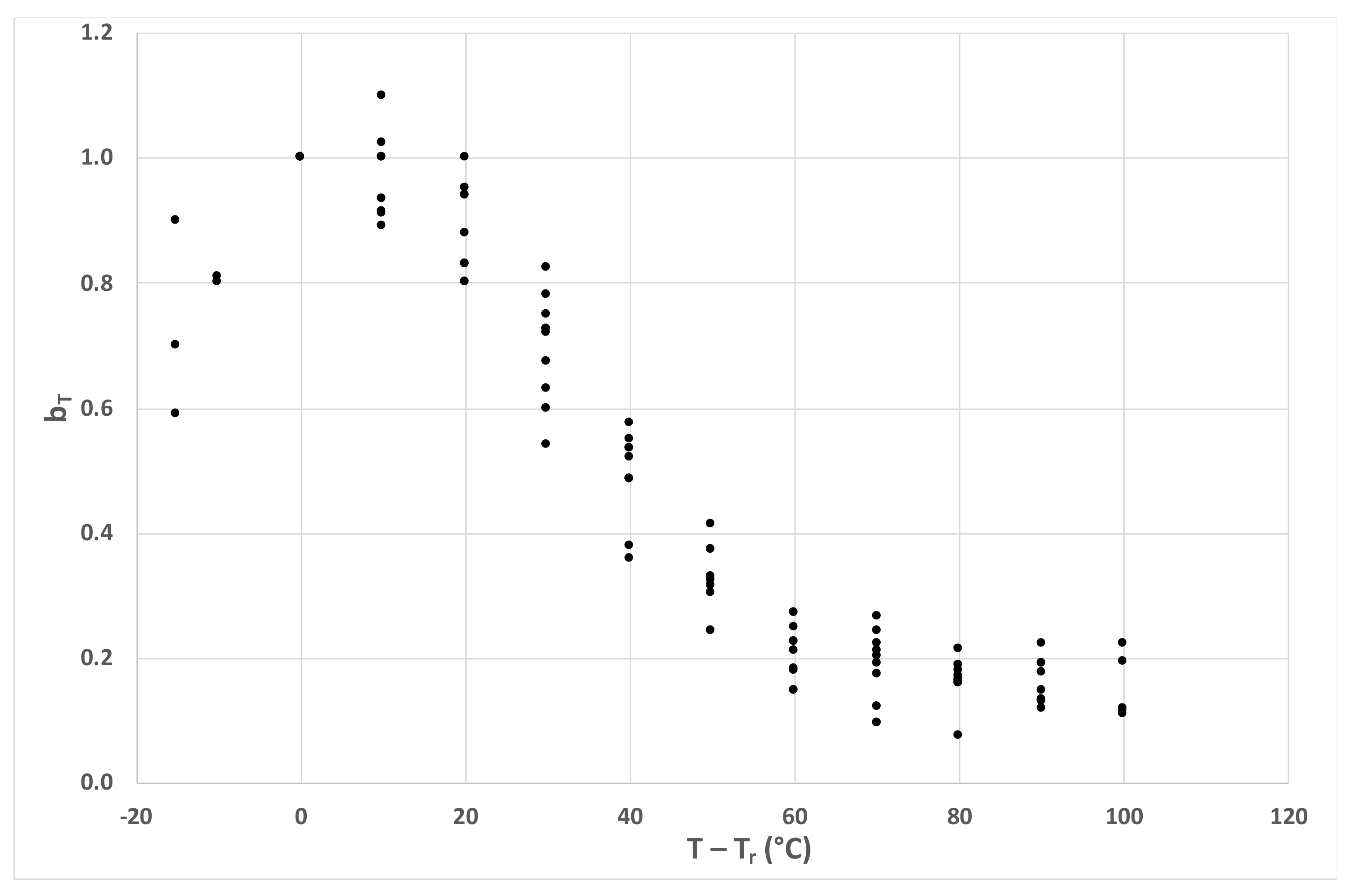
With regard to the vertical shift, all the samples showed a similar behaviour that does not correlate with aging. The variation in the vertical shift factors with temperature is reported in Figure 5, where all the data corresponding to the B and LS-B at 0, 25, 40, 65, and 90 h of PAV are represented with the same symbol, in order to visualize the common trend.

3.2. Apparent Molecular Weight Distributions

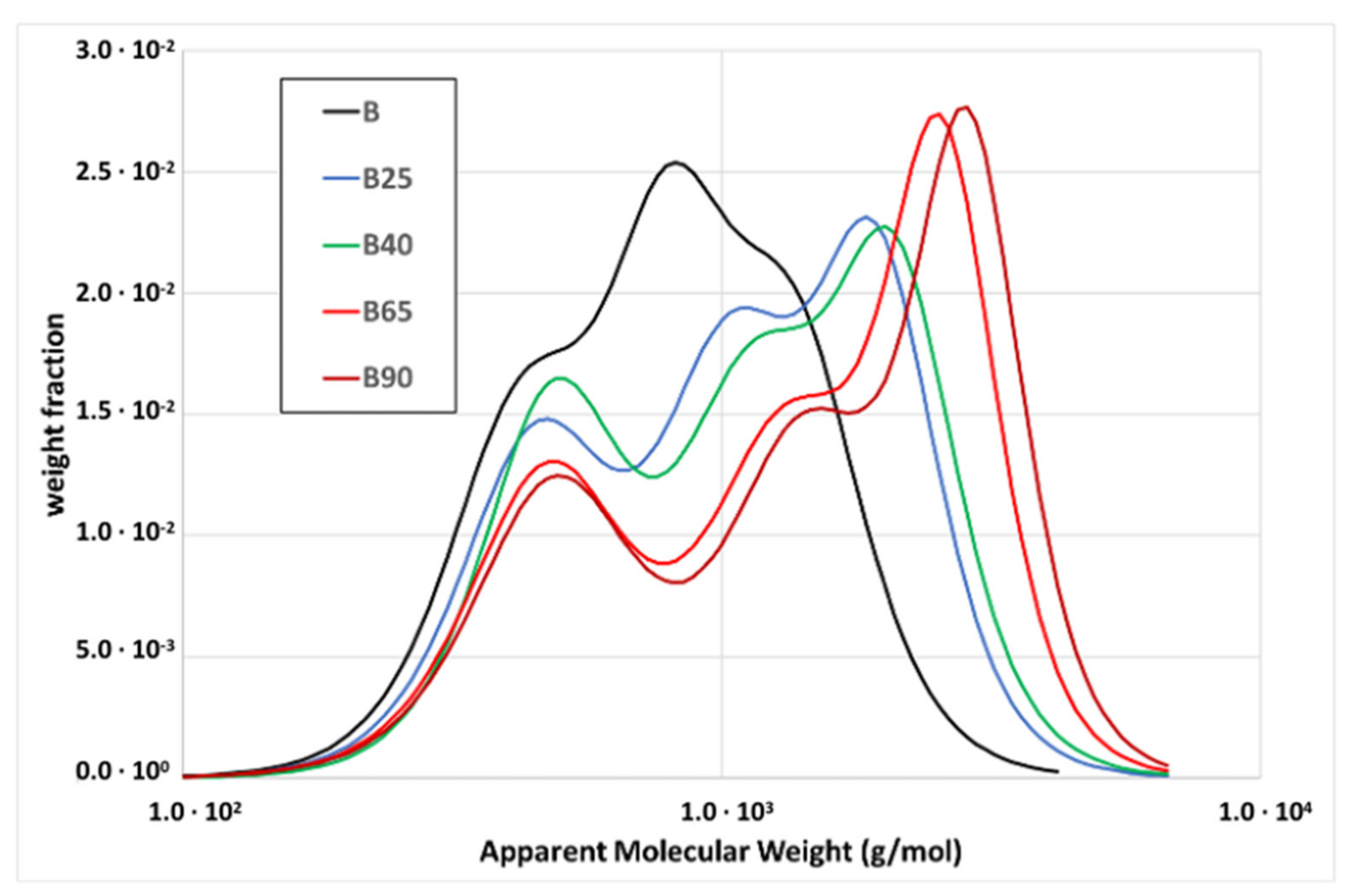
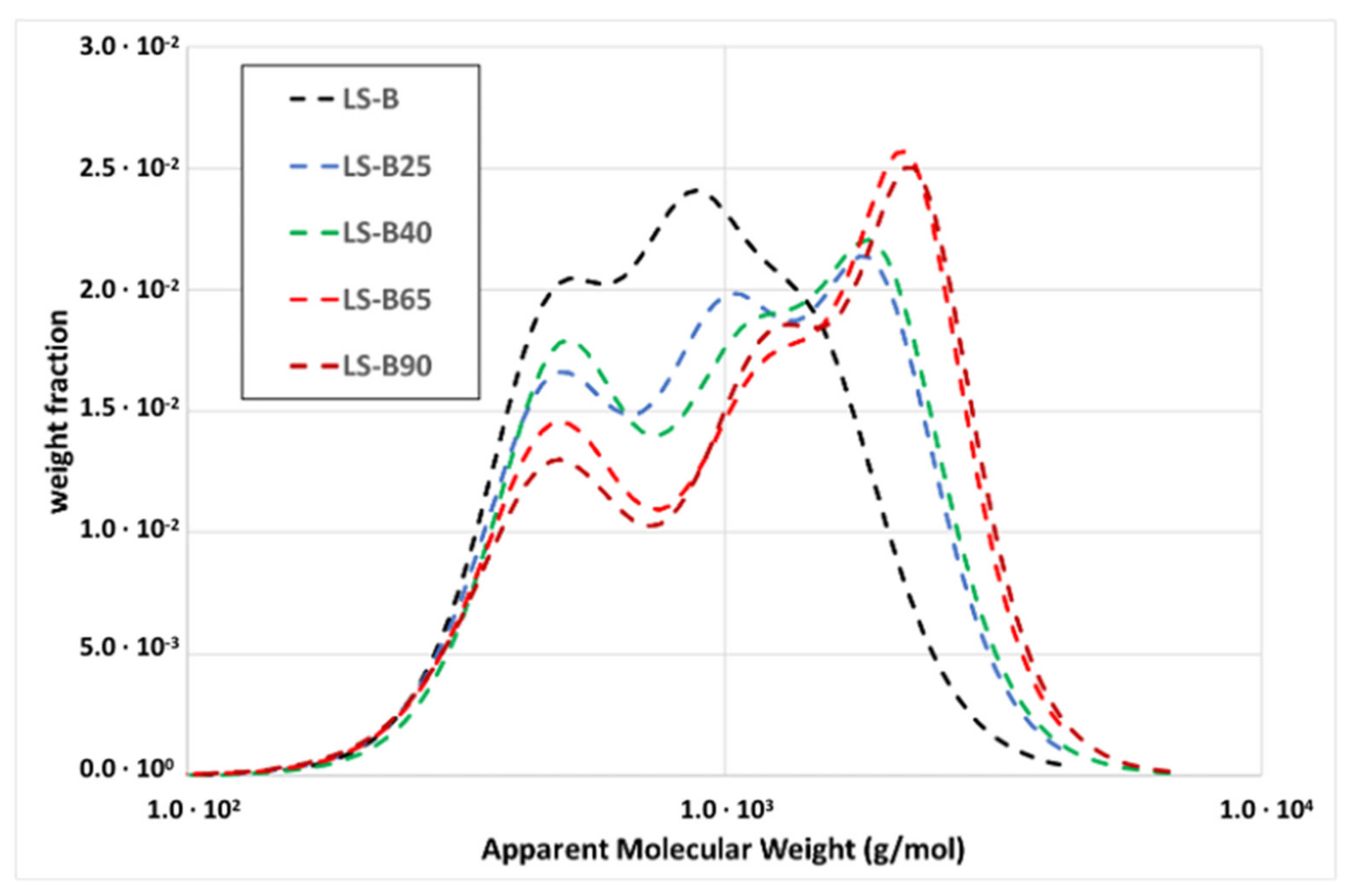
As described in the previous section, from the rheological data, the AMWD were determined by applying the so-called “δ-method” [5,39], also used to evaluate the binder aging based on the evolution of such a distribution [40]. Figure 6 and Figure 7 show the distributions at all levels of aging for binders B and LS-B, respectively. All curves were obtained by applying the δ-method, after fitting the master curves with the 2S2P1D model (model parameters are listed in

Table 3. The 2S2P1D model’s parameters.

Sample	G0 (Pa)	G∞ (Pa)	α	β	τ	k	h
B	1.0 · 10−8	5.82 · 108	0.0350	1.07 · 104	1.19 · 10−4	0.666	0.312
B25	1.0 · 10−8	5.82 · 108	0.0180	1.58 · 105	3.48 · 10−4	0.633	0.305
B40	1.0 · 10−8	5.82 · 108	0.0191	1.35 · 105	1.03 · 10−3	0.639	0.323
B65	1.0 · 10−8	5.82 · 108	0.0105	2.32 · 106	7.50 · 10−4	0.595	0.292
B90	1.0 · 10−8	5.82 · 108	0.0084	5.50 · 106	1.15 · 10−3	0.590	0.287
LS-B	1.0 · 10−8	5.82 · 108	4.68	6.05 · 101	5.53 · 10−2	0.338	0.680
LS-B25	1.0 · 10−8	1.83 · 108	6.13	2.05 · 102	2.03 · 10−1	0.319	0.648
LS-B40	1.0 · 10−8	5.82 · 108	0.0253	5.53 · 104	1.25 · 10−3	0.649	0.334
LS-B65	1.0 · 10−8	5.82 · 108	0.0153	4.14 · 105	8.44 · 10−4	0.615	0.304
LS-B90	1.0 · 10−8	3.70 · 108	0.0114	6.88 · 105	7.78 · 10−4	0.615	0.290

).

In both cases, there is an evident shift of the right part of the distributions toward higher molecular weights; this being an immediate confirmation that the dispersion index increases with aging, as suggested by the |G_c| values. Moreover, the shape of the AMWD shows two other important changes related to aging. First, the low MW peaks decrease in intensity, while the high MW peaks increase; second, the overlapping of the peaks diminishes, introducing a shape shift from a unimodal to a multi-modal curve, according to aging time. The latter is a direct consequence of the increase in DI, which means a wider distribution. Again, a graph comparing the two binders helps understanding the effect of the clay (Figure 8).

The AMWD is affected by both the molecular weight and the interactions that determine the aggregation of the molecules. In the unaged conditions, the B and LS-B curves are similar but not completely superposed, thus confirming the already observed influence of layered silicate on the bitumen structure [41,42]. Nevertheless, the binders B and LS-B start from similar apparent distributions, which progressively diverge with increasing aging. At 25PAV, the LS-B binder already shows a reduced dependence on aging with respect to the B binder. Then, at higher levels of aging, the B distribution clearly includes molecules or aggregates of higher dimensions.

The shift toward higher M_w can be quantified by calculating the number (M_n) and weight (M_w) average molecular weights, and the dispersion index, which has a direct link with the square value of the variance (σ²) of the distribution:

$$DI=\frac{M_w}{M_n}=\frac{{\sigma }^2}{M_n^2}+1$$

(18)

Based on these quantities, we can define the following aging indexes:

$$A{I}_n=\frac{M_{n,a}}{M_{n,u}}\hspace{1em}\hspace{1em}A{I}_w=\frac{M_{w,a}}{M_{w,u}}\hspace{1em}A{I}_{DI}=\frac{D{I}_a}{D{I}_u}$$

(19)

The numerical values for the two binders are reported in

Table 4. Average molecular weights, dispersion, and aging indexes for B and LS-B.

	B						LS-B
PAV	Mn (g/mol)	Mw (g/mol)	DI	AIn	AIw	AIDI	Mn (g/mol)	Mw (g/mol)	DI	AIn	AIw	AIDI
0	743	784	1.06	1.00	1.00	1.00	794	836	1.05	1.00	1.00	1.00
25	942	1013	1.08	1.27	1.29	1.02	923	986	1.07	1.16	1.18	1.02
40	1002	1079	1.08	1.35	1.38	1.02	962	1029	1.07	1.21	1.23	1.02
65	1167	1279	1.10	1.57	1.63	1.04	1050	1135	1.08	1.32	1.36	1.03
90	1265	1394	1.10	1.70	1.78	1.04	1090	1180	1.08	1.37	1.41	1.03

.

All indexes confirm the anti-aging effect of the clay and the most sensitive index seems to be AI_w.

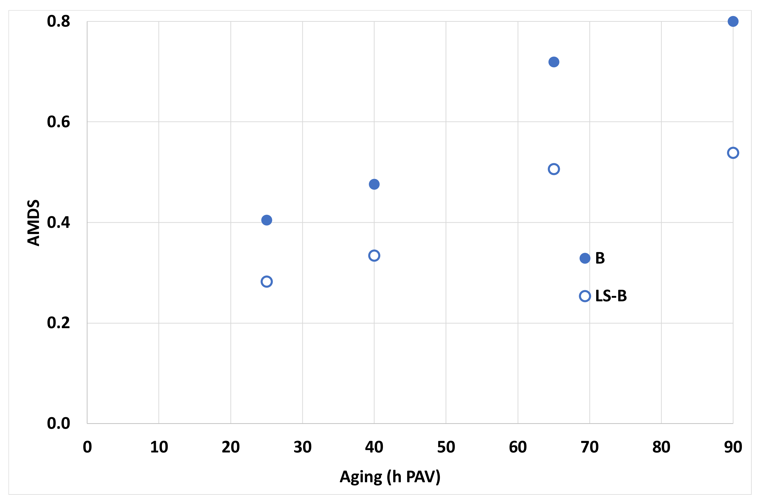
One of the disadvantages of the indexes defined in Equation (19) is that they refer to a single data point. The first and second give an idea of the shift of the curve toward higher MW. The third one is related to the variance of the curve, but it has not a clear physical meaning when the curve has a complex shape, such as the AMWD, after aging. As it was for the master curves, we need something that may take into account the changes in the whole curve. One parameter that may help is the Aging Molecular Distribution Shift (AMDS) proposed by Themeli et al. [39]:

$$AMDS={{\displaystyle \int }}_0^{\infty }\left|f_a-f_u\right|dlogMW$$

(20)

where f_a and f_u are the weight fractions in the AMWD. In other words, the AMDS gives the area of the absolute value of the difference between the distributions obtained before and after aging. Both horizontal and vertical shifts as well as variations in shape affect this parameter. Figure 9 shows that AMDS is always higher for B and the difference with respect to LS-B increases with aging.

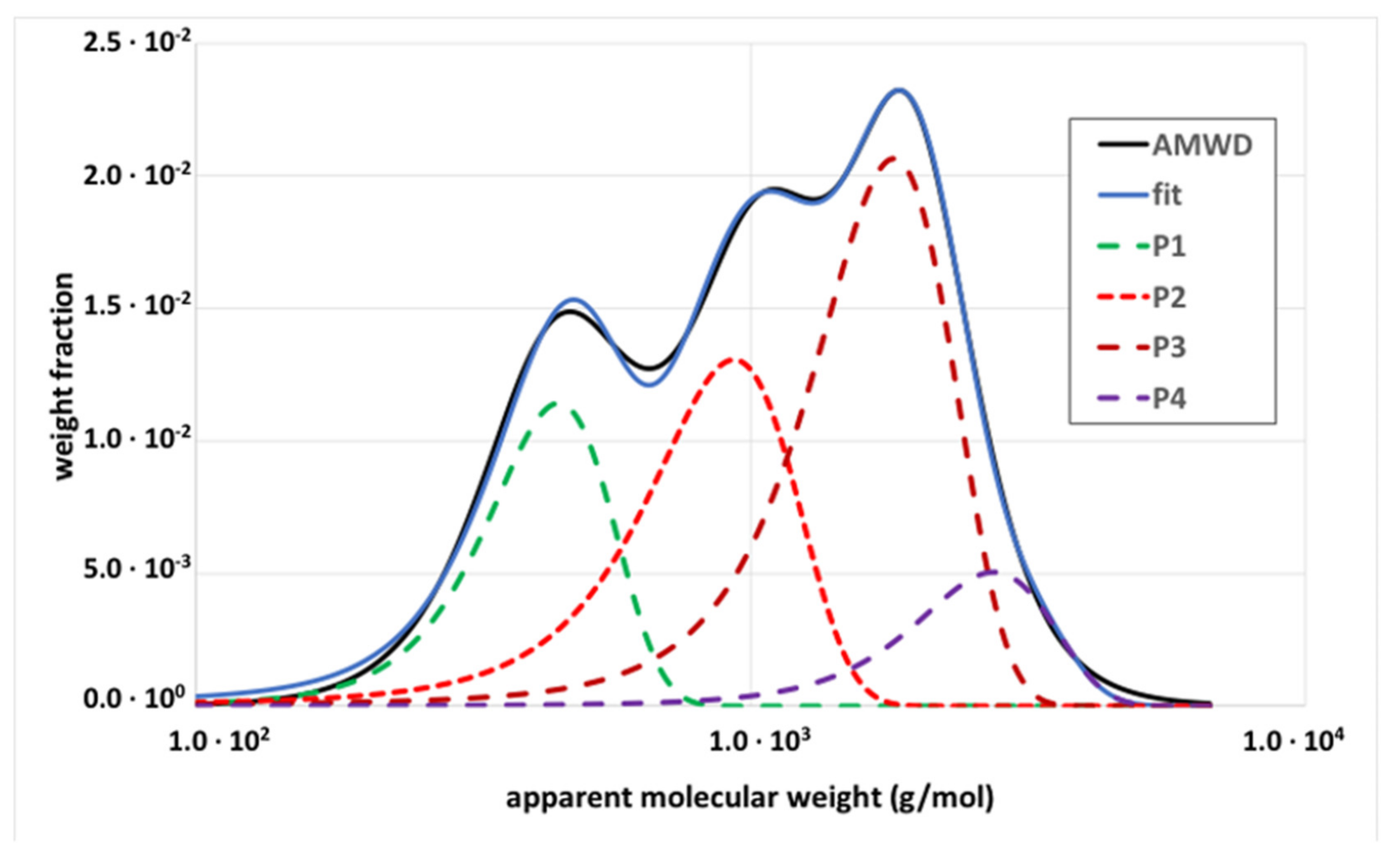
Another interesting aspect of the AMWD is that with increasing aging, the main peaks of the distribution separate one from each other. This suggests analysing the peaks individually, by means of a simple deconvolution procedure. As proposed by Krolkral et al. [40], the AMWD were fitted with four Gaussian functions associated with populations with different molecular weights. As an example, Figure 10 shows the four populations (named P1 to P4) for the B25 binder.

Table 5. Percentage area of the P1–P4 populations and related aging index for the B and LS-B binders.

Sample	P1		P2		P3		P4		${\displaystyle \frac{(\mathit{P}3+\mathit{P}5)}{(\mathit{P}1+\mathit{P}2)}}$	AIP
	MW (g/mol)	Area (%)	MW (g/mol)	Area (%)	MW (g/mol)	Area (%)	MW (g/mol)	Area (%)
B	418	7.6	752	26.1	1257	42.4	1937	24.0	1.97	1.00
B25	451	6.8	933	18.7	1811	54.7	2742	19.9	2.93	1.49
B40	490	7.7	1003	16.8	1947	54.6	2965	20.8	3.08	1.56
B65	485	5.8	1183	17.0	2466	57.3	3529	19.9	3.37	1.71
B90	501	5.4	1312	17.9	2772	55.7	3889	21.1	3.29	1.67
LS-B	462	9.0	791	24.0	1330	41.3	2054	25.7	2.03	1.00
LS-B25	471	7.4	910	20.0	1757	50.5	2663	22.1	2.65	1.31
LS-B40	496	8.5	952	16.8	1797	52.0	2742	22.7	2.95	1.46
LS-B65	484	6.8	1049	16.9	2086	56.8	3067	19.5	3.22	1.59
LS-B90	479	6.0	1102	18.4	2175	56.3	3219	19.3	3.09	1.52

summarises the molecular weight (g/mol) corresponding to the peak and the relative quantities of the four populations, calculated as the integral of the relative Gaussian peak.

All peaks shift toward higher molecular weights, this being more accentuated for the P3 and P4 peaks. With respect to the relative quantities, only P3 registers an increase due to aging while the other ones diminish more or less evidently. Moreover, the most significant variations usually appear in the first aging step. However, due to peaks overlapping, it is difficult to evaluate aging from the analysis of the individual populations. Therefore, the populations were grouped in light (P1 + P2) and heavy (P3 + P4) weight fractions and the following aging index (included in Table 5) was defined:

$$A{I}_P=\frac{{\left[\frac{\left(P3+P4\right)}{\left(P1+P2\right)}\right]}_a}{{\left[\frac{\left(P3+P4\right)}{\left(P1+P2\right)}\right]}_u}$$

(21)

AI_P takes into account the relative quantities of the high and low MW populations and gives a further confirmation of the positive effect of clay as an anti-aging additive.

3.3. High-Performance Thin-Layer Chromatography

It is obvious that the four populations obtained with the deconvolution differ from the well-known SARA fractions that derive from a fractionation with solvents of different polarity [29]. Nevertheless, since there is an increase in molecular weight and state of aggregation that parallels the increase in polarity, it is interesting to investigate if the four populations and SARA fractions somehow correlate. For this reason, we can here introduce the only “not-rheological” data, which are the results of the HPTLC analysis (Table 5). The evolution of the composition clearly individuates the fractions most affected by aging. Saturates and asphaltenes do not change significantly, at least from a quantitative point of view. In contrast, a consistent number of aromatic molecules move toward the resin family due to oxidation. It is worth nothing that for aromatics and resins, the variation in composition is higher in the presence of clay. This seems to be in contrast with the anti-aging effect of clay observed until now through rheological data. However, if we define an aging index (AI_SARA) similar to AI_P, the result is consistent with the previous ones, thus indicating that the aging indexes must take into account the whole composition.

This is clarified in the last three columns of

Table 6. SARA fractions from HPTLC.

Sample	Saturates (%)	Aromatics (%)	Resins (%)	Asphaltenes (%)	AIar	AIres	AISARA
B	10.7	50.1	25.0	14.2	1.00	1.00	1.00
B25	9.8	46.0	31.8	12.4	0.72	1.29	1.48
B40	10.9	43.5	33.4	12.2	0.65	1.35	1.72
B65	10.6	39.9	37.4	12.1	0.64	1.29	1.56
B90	9.2	40.0	38.5	12.3	0.69	1.31	1.67
LS-B	10.1	54.2	22.1	13.6	1.00	1.00	1.00
LS-B25	10.1	50.4	27.6	11.9	0.83	1.22	1.31
LS-B40	10.3	49.4	29.1	11.2	0.70	1.26	1.45
LS-B65	10.5	44.3	34.3	10.8	0.70	1.38	1.59
LS-B90	10.4	40.9	38.1	10.6	0.77	1.36	1.53

that report the following aging indexes:

$$A{I}_{ar}=\frac{{\left(ar\%\right)}_a}{{\left(ar\%\right)}_u}\hspace{1em}\hspace{1em}A{I}_{res}=\frac{{\left(res\%\right)}_a}{{\left(res\%\right)}_u}\hspace{1em}\hspace{1em}A{I}_{SARA}=\frac{{\left[\frac{\left(res\%+asph\%\right)}{\left(sat\%+ar\%\right)}\right]}_a}{{\left[\frac{\left(res\%+asph\%\right)}{\left(sat\%+ar\%\right)}\right]}_u}$$

(22)

where sat, ar, res, and asph indicates saturates, aromatics, resins, and asphaltenes, respectively. The indexes that refer to a single population may give misleading information with regard to the global evolution with aging.

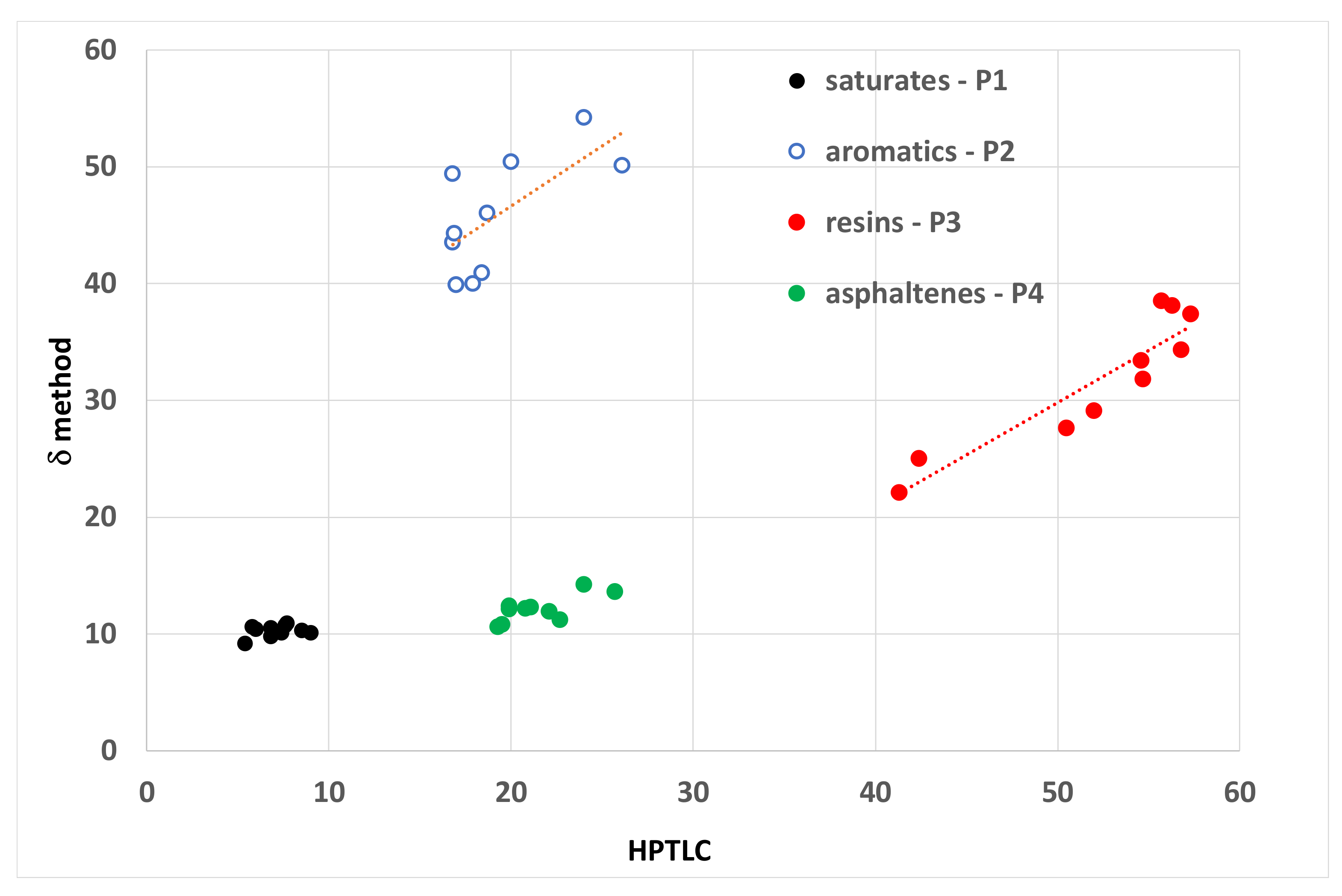
Finally, in order to better visualize the affinity between the two kinds of populations, Figure 11 gives a picture of the above-supposed correlation by reporting the data of Table 6 without distinction between the B and LS-B binder. The x-axis is the relative percentage obtained with HPTLC and the y-axis is the percentage calculated with the δ-method. The image confirms the parallelism between the δ-method and HPTLC families. Saturates-P1 and asphaltenes-P4 do not change significantly, while the P2-aromatics and P3-resins populations have a higher sensitivity to aging. This is interesting food for thought. The prefix “A” in AMWD stands for apparent and is introduced to distinguish between data collected in solution (for example with gel permeation chromatography) and in bulk (rheology). Following the same reasoning, the four populations can be named A-MGD, which stands for apparent molecule groups dynamics and motions, which give an idea of how the composition/aggregation of the molecules’ dynamic and motion changes with aging.

3.4. Relaxation Spectrum

The relaxation spectrum, usually indicated as H($\tilde{\tau }$), is one of the most important rheological functions, since once it is known, it allows calculating any other viscoelastic function and vice versa [11]. For this purpose, a number of algorithms has been proposed to obtain H($\tilde{\tau }$) from the master curve of a viscoelastic function [25,38,43,44,45]. Moreover, since it describes a distribution of relaxation times, H($\tilde{\tau }$) can be viewed as an indirect measurement of the MWD [46] and specific relationships have been proposed for polymers [38,47,48] and bituminous binders, thus providing an alternative to the δ-method [38]. For all these reasons, H($\tilde{\tau }$) can be used to characterize the aging of the binders [38,49]. Naderi et al., observed a horizontal shift of the relaxation spectra towards higher relaxation times and suggest the use of the mean value, variance, and skewness of the spectra to characterize its evolution with time [50]. Zhao et al., derived an indicator to evaluate the effect of rejuvenators directly from H($\tilde{\tau }$) [51].

As described in the materials and method section, the relaxation spectra were derived from the 2S2P1D model and in what follows, they are reported on a logarithmic scale, where the range of the x-axis corresponds to experimental data. In other words, the 2S2P1D model in this case is used only in the frequency range covered by the experimental master curve and there is no extrapolation of the data outside that range. Therefore, the reported spectra represent only a portion of the usual asymmetric bell shape corresponding to a full range of relaxation times. This portion is located after the bell peak, and thus the curves decrease monotonically with the relaxation time. For this reason, the variance and skewness are not very useful parameters. Nevertheless, the shift of the spectra toward higher relaxation times is clearly visible as well as how the clay reduces this shift. 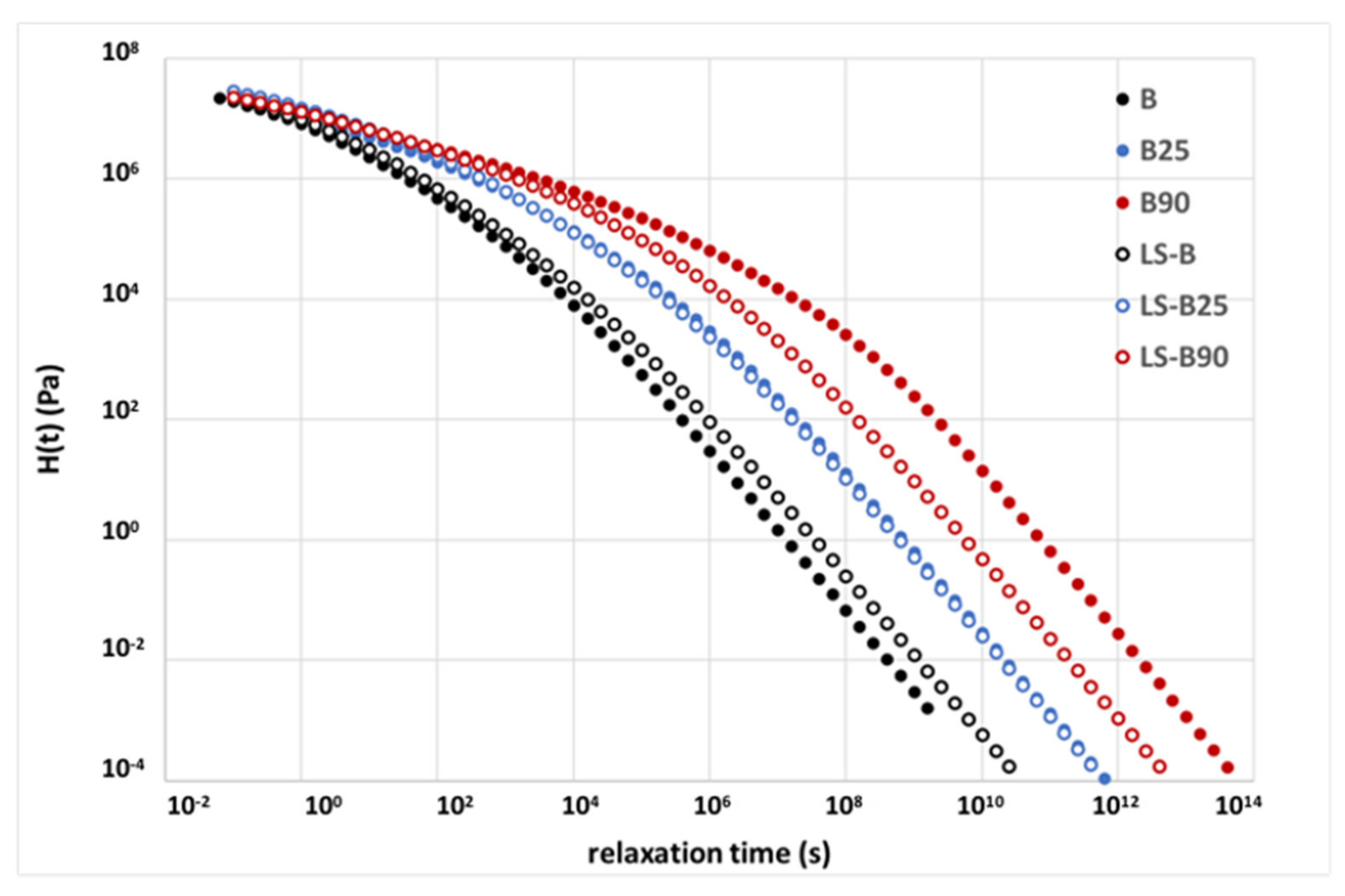Figure 12 and Figure 13 show the relaxation spectra for the B binder at different levels of aging and the usual comparison with the LS-B binder, respectively. For both binders, the relaxation spectra converge to similar values at low relaxation times and show the main differences in the right-hand side of the spectra. This is consistent with the already observed variations in MWD. The low MW molecules (lower relaxation times) are less affected by the oxidation, while the other molecules change their composition, favouring a higher degree of aggregation. This determines the shift to the right of both the AMWD and H($\tilde{\tau }$) curves.

Since in a logarithmic plot all the relaxation spectra appear parallel at high relaxation times, an aging index could be defined in order to take into account this horizontal shift of the right-hand side of the curves:

$$A{I}_H=\frac{{\left(\log \tilde{\tau }\right)}_a}{{\left(\log \tilde{\tau }\right)}_u}$$

(23)

where $\tilde{\tau }$ indicates the numerical value of time expressed in seconds and the index is evaluated at any H($\tilde{\tau }$) in the range were the behaviour is linear in the logarithmic plot, which means below approximately 100 Pa. As an example, the vertical arrows in Figure 12 indicate the values of τ for B and B25 corresponding to H($\tilde{\tau }$) = 1 Pa. The obtained values are reported in

Table 7. Aging indexes from the relaxation spectra.

	B	B25	B40	B65	B90	LS-B	LS-B25	LS-B40	LS-B65	LS-B90
AIH	1.00	1.29	1.32	1.48	1.60	1.00	1.18	1.19	1.28	1.32

.

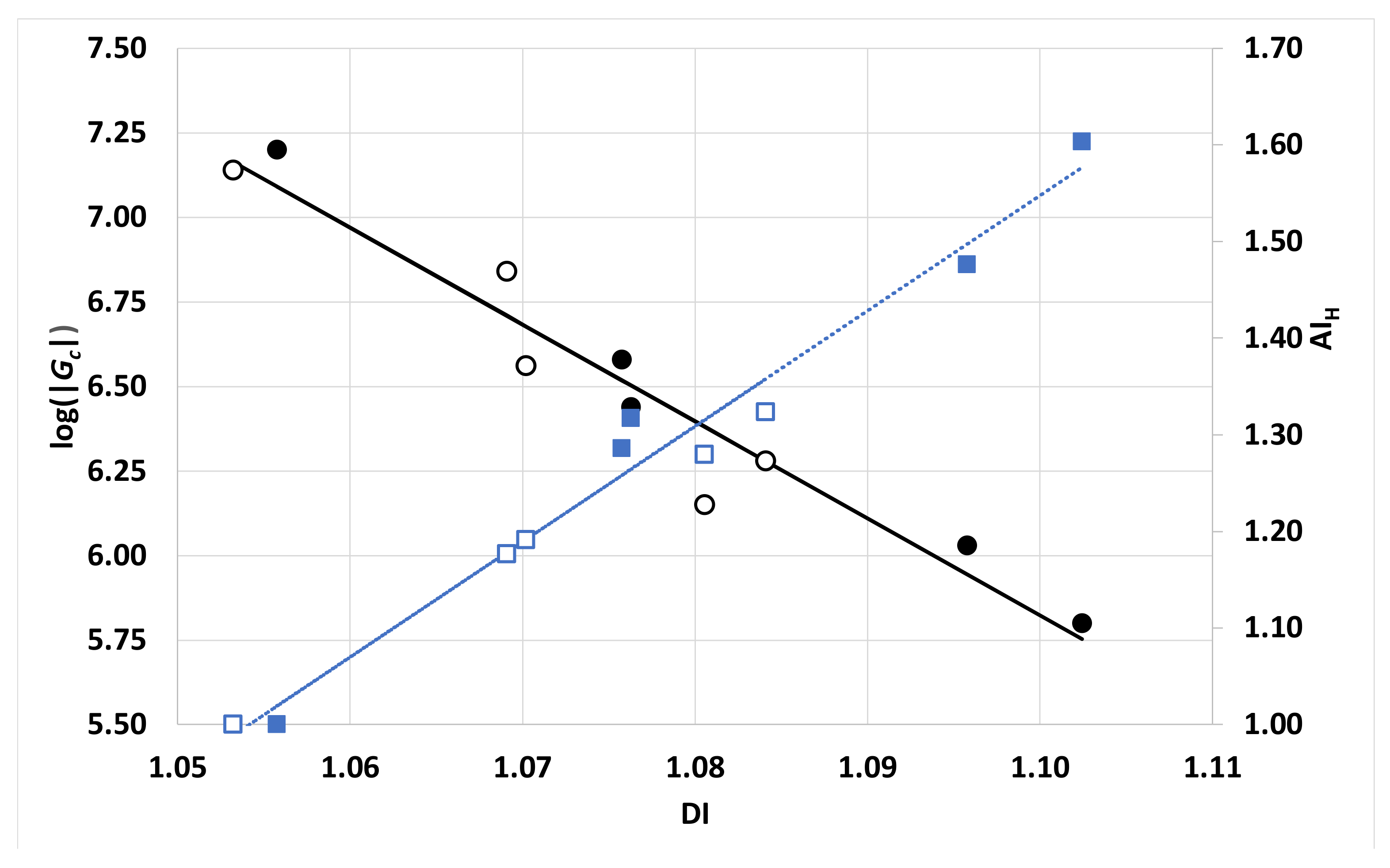
Eventually, it is interesting to correlate the data obtained from the master curves, AMWD, and relaxation spectra. Given the abovementioned connection between the crossover modulus and the dispersion index, their values are represented in a log(|G_c|)-DI space (Figure 14, left y-axis), which clearly confirms the correlation and suggests a linear dependence between the two quantities. Even better is the linear correlation for the data indicated by squares, which refer to the right y-axis and represent the AI_H index.

A simple linear regression, including both B and LS-B data, gives a coefficient of determination R² = 0.94 and 0.98 for |G_c| and AI_H, respectively.

4. Conclusions

In the characterization of bituminous binders, rheology is the leading way because it is related to many properties, such as rutting, elastic recovery, fatigue cracking, and so on. In particular, it is common practice to construct master curves of the linear viscoelastic functions by applying the time–temperature superposition principle to frequency sweep data obtained in the isothermal tests. In this way, a single picture representing the behaviour of the binder from the glassy to the liquid state can be obtained. Such curves contain much information that may be linked to the molecular structure of the material and used to compare the aged and unaged states. The master curves can be used as they are or after transformation into other viscoelastic functions, such as the relaxation spectrum, or into an apparent molecular weight distribution. In all these cases, transforming the information contained in a curve into an aging index or into a structural model is not an easy task and several procedures may be adopted. In this work, a list of many aging indexes, either new or previously suggested in the dedicated literature, is presented in order to compare their sensitivity to ageing and to underline their physical meaning. Moreover, an analysis of the evolution with aging of the three representations (master curves, apparent molecular weight distribution, and relaxation spectrum) allowed underlining some interesting interconnections. The first one is between |G_c| and H($\tilde{\tau }$) with the dispersion index calculated from the AMWD. Moreover, an interesting link between the four populations derived with the deconvolution procedure applied to the AMWD and the four SARA fractions obtained with HPTLC was observed. If the AMWD is fitted with four Gaussian peaks, there is a qualitative similarity in the evolution with aging of the four couples P1-saturates, P2-aromatics, P3-resins, and P4-asphaltenes. This suggested the use of a new acronym A-MGD (apparent molecules groups dynamics and motions). As a final consideration, we can affirm that the apparent molecular weight distribution is probably the most useful representation, because with aging it undergoes considerable shifts and variation in shape and may give both good aging indexes and insight into the binder composition. As expected, all the collected data and aging indexes confirm that clay has an anti-aging effect that remains appreciable even after severe artificial aging, as well as a direct effect on the aggregation dynamics of the binder molecules.