A Semi-Empirical Fluid Dynamic Model of a Vacuum Microgripper Based on CFD Analysis

Abstract

Vacuum microgrippers are devices used to handle and manipulate small objects. Despite their simple working principle and low cost, they show low efficiency in detaching performance, especially when the object to be grasped is very small. In this work, a particular design for vacuum microgrippers with an incorporated automatic release tool is considered. The final goal of this study was to present a numerical model that can supply reliable estimates of the aerodynamic force acting on the release tool and of the air flow rate inside the gripper as a function of geometric parameters and the outlet pressure value. A complete CFD analysis of a simplified model of the device is presented. Grid independence analysis was also performed to define a suitable grid and guarantee a good trade-off between accuracy and computing time. According to Design of Experiments (DOE) techniques, 81 simulations were performed, changing the values of the outlet pressure ($p_2$), the body inner diameter (D), the lateral holes’ diameter (d) and the releasing mass length (L). Every design variable could assume three different values. Linear regression, based on the least square method, was employed to determine mass flow rate and lifting force empirical correlations.

1. Introduction

Since the early 2000s, the exponential growth of micro-electromechanical systems (MEMS) has been made possible by increasingly low production costs, which paved the way for the design of small devices that are able to manipulate and assemble very small objects (at the micro and nanoscale range) with speed and precision, called microgrippers. The use of microgrippers has rapidly extended to other sectors—for example, biotechnology [1] and microsurgery [2]. The different kinds of microgrippers used in micromanipulation exploit the same gripping strategies already employed for years in macromanipulation. In the field of macromanipulation, which involves handling objects larger in size (greater than 1 µm), mechanical grippers are widely used. In these devices, the lifting force on the object can be applied using jaws (impactive gripper) [3] or penetrating and deforming the surface of the object (ingressive gripper) [4]. The use of mechanical grippers in microhandling has proved challenging: it is difficult to scale down the kinematics used to move jaws or gripper arms and to achieve consistent acceptable mechanical performance [5,6]. According to the specific application, so-called astrictive microgrippers are more suitable and offer the best gripping performance. They can use both contact and contactless techniques based on different actuation principles: magnetic fields [7], electrostatic forces [8] and vacuum suction [9]. Among these, vacuum microgrippers have become widespread in the electronic industry due to a simple working principle and low cost, coupled with fast and effective handling. However, as contact grippers, they have to overcome non-negligible adhesion forces between the gripper, and the handled object that, at this sort of range, can prevent the release of the object. Different strategies have been proposed to overcome this issue and to assist with the object detachment. So-called passive release strategies aim to reduce the forces acting at the microscale: coating the gripper surface with a conductive layer connected to the ground to reduce the electrostatic force [8] is an example. Active release strategies provide supplementary forces to overcome adhesion, such as vibration [10], positive pressure pulse [9] or electric fields [11]. The goal of this paper is to present the CFD analysis of vacuum microgrippers with an integrated automatic detaching tool (releasing mass) [12]. Simulations have been performed for 27 different gripper configurations, which were defined according to Design of Experiments (DOE) techniques. The values of three geometrical gripper parameters were changed in the simulations. Since each configuration was investigated for three outlet pressure values, 81 CFD simulations were carried out. CFD results were analyzed in order to find out how gripper geometry affects the gripping performance. Empirical correlations based on numerical results are proposed to predict the air mass flow rate inside the gripper and the aerodynamic force exerted on the releasing mass. The correlations should speed up the design phase.

2. Material and Methods

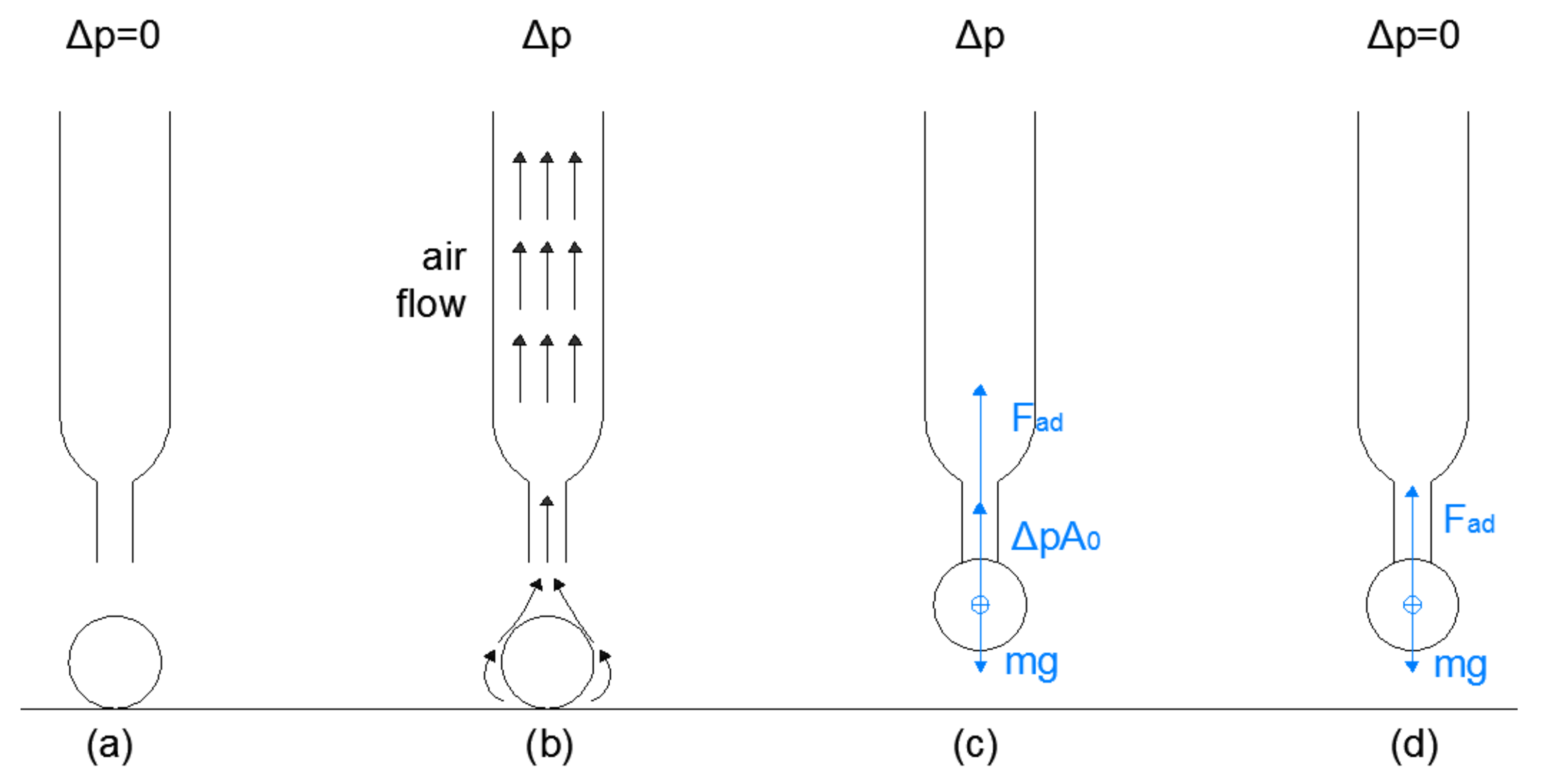
2.1. Vacuum Microgripper and Its Working Principle

Classic vacuum microgrippers consist of two parts: a hollow body and a thin cannula (Figure 1).

The three manipulation tasks (grasping, handling, releasing) are carried out through a simple working principle.

When a pressure difference, Δp, between the inflow section and the volume inside the gripper is created by a vacuum pump connected to the gripper, airflow is forced through the cannula and inside the device, generating a suction force that picks up the object (grasping phase) (Figure 1b).

When the object sticks against the cannula end (handling phase) (Figure 1c), the gripper must provide a continuous handling force ($F_H$) that, according to Equation (1), must be sufficiently high to overcome the weight force (mg) minus the adhesion forces ($F_{AD}$):

$$F_H=\Delta p{A}_0\ge mg-F_{AD}$$

(1)

where $A_0$ is the cannula’s cross-sectional area, m the object mass and g the gravitational acceleration.

The releasing phase begins when Δp = 0. However, the weight force is not often enough to strip off the object due to high adhesion forces (i.e., Van der Waals, electrostatic, surface tension) acting between the grasped object and the cannula’s surface (Figure 1d). When the objects to manipulate are very small in size (less than 10 µm), the importance of adhesion forces (proportional to the object surface) arises and can be dominant over gravitational and inertial forces (proportional to the object volume) (Figure 2).

In order to overcome this issue, some authors [12] patented a different kind of vacuum microgripper, equipped with an automatic release tool. A releasing mass (in red in Figure 3), combined with a thin needle, is inserted inside the gripper body and can move up and down in the axial direction. A mechanical stop (not shown in figure) limits the vertical displacement of the releasing mass. In addition, two lateral holes are provided on the lateral gripper body surface to enhance airflow inside the device and to allow the releasing mass to be lifted also during the handling phase.

The aerodynamic force ($F_M)$ acting on the releasing mass during the device operation (grasping and handling phase) (Figure 3b,c) is the sum of two contributions, according to the following equation:

$$F_M=F_P+F_V$$

(2)

The pressure force ($F_P)$ is generated by the difference between the average pressure acting on the upstream ($p_{sx})$ and the downstream ($p_{dx})$ base of the releasing mass ($A_c)$ and is defined as

$$F_P\cong \left(p_{sx}-p_{dx}\right)A_c$$

(3)

The viscous force ($F_V)$ is generated by shear stresses (${\tau }_w)$ acting on the releasing mass lateral surface ($A_L)$ in the annulus region, and is defined as

$$F_V={\int }_{A_L}{\tau }_{w}dA$$

(4)

When the pressure difference is removed, i.e., Δp = 0, the releasing mass moves downward and helps with object detachment (see Figure 3d). As shown in [14], this integrated release tool significantly improves the device’s release effectiveness. Greater values of the releasing tool mass (M) allow one to overcome high adhesive forces, especially for small objects, according to the following equation:

$$\left(m+M\right)g>F_{AD}$$

(5)

The value of M must be carefully chosen (see Figure 3e) as follows:

$$M\le \frac{F_M}{g}$$

(6)

to ensure that $F_M$ is sufficiently high to correctly lift the releasing tool and guarantee proper device operation. The value of $F_M$ is closely related to the air flow field that develops inside the gripper, which in turn, is strictly affected by the device geometry. To find out how the geometry influences $F_M$, a complete CFD analysis was performed on a simplified gripper model, described in the next section.

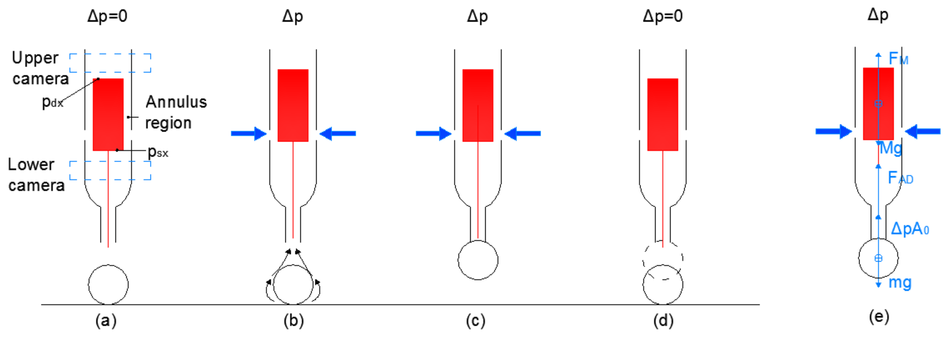
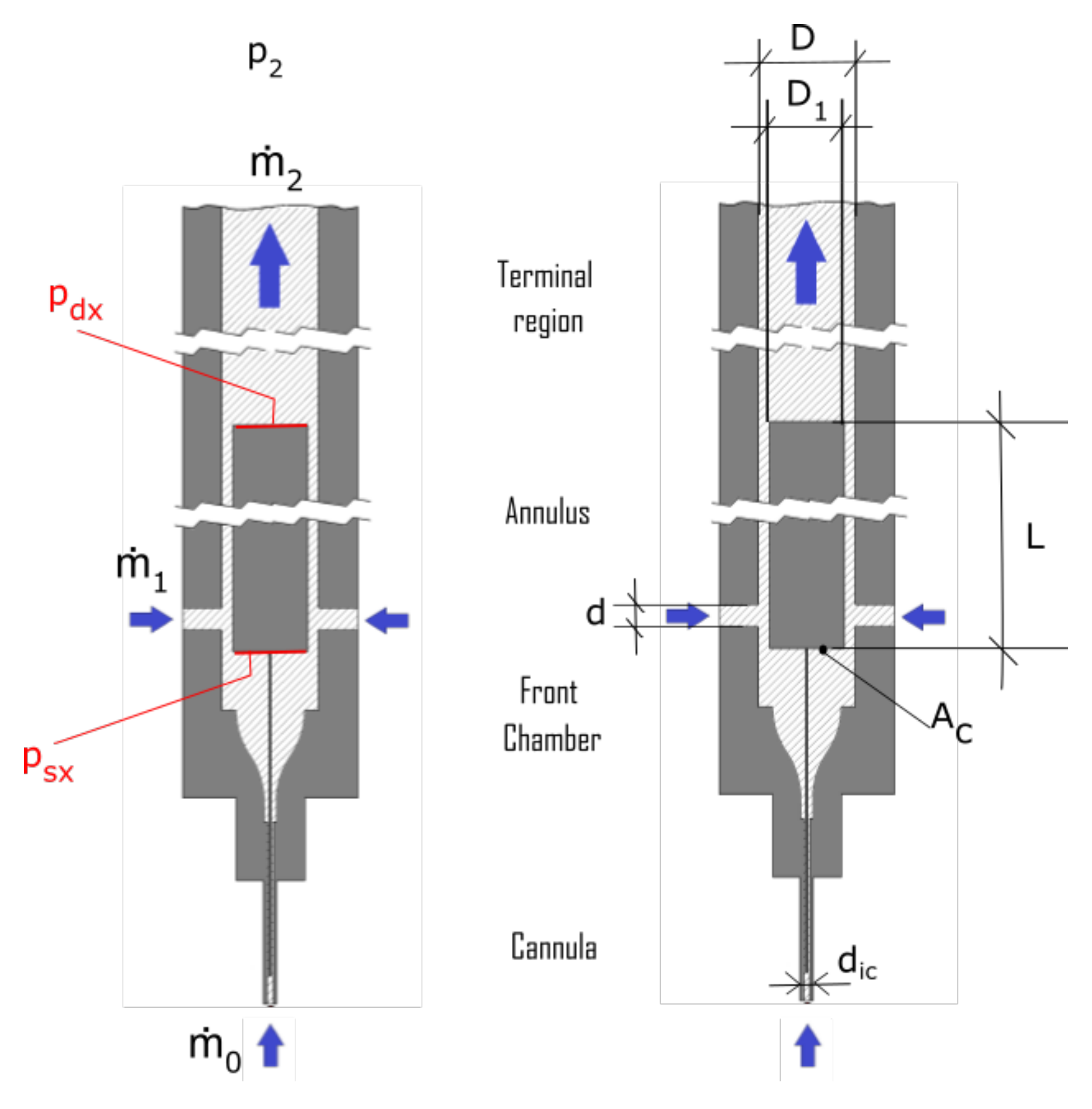
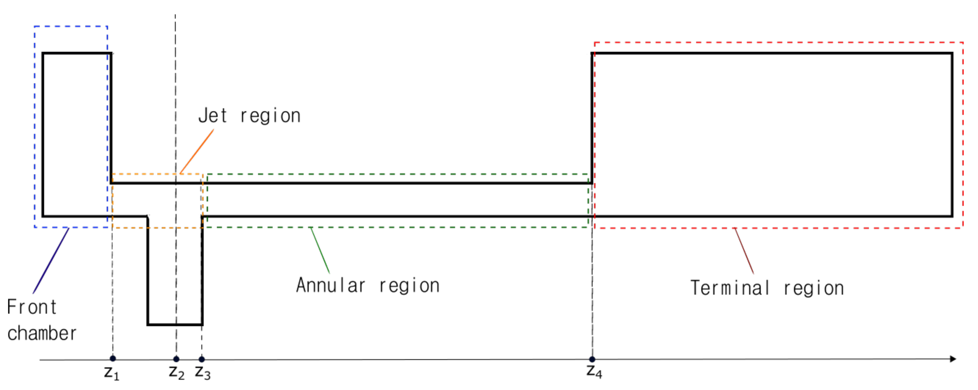
2.2. Simplified Gripper Model

Figure 4 shows all the physical and geometrical quantities considered in this study.

The total air mass flow rate through the device (${\dot{m}}_2$) is given by the sum of two contributions: the air flow through the cannula (${\dot{m}}_0$) and the incoming air from the lateral holes (${\dot{m}}_1$).

$${\dot{m}}_2={\dot{m}}_0+2{\dot{m}}_1$$

(7)

However, it is reasonable to expect that the air flow through the cannula (${\dot{m}}_0$) is negligible, i.e., ${\dot{m}}_2\approx 2{\dot{m}}_1,$ since the cannula’s inner diameter ($d_0)$ is significantly smaller than the side holes’ diameter (d). Neglecting the air flow (${\dot{m}}_0$) does not significantly affect the total flow rate through the device (${\dot{m}}_2$), nor the aerodynamic force on the releasing mass ($F_M$), nor the flow fields inside the gripper. This was confirmed by the numerical results obtained in a previous work [15]. Therefore, the computational model used for the CFD analysis takes into consideration only the gripper body, according to the simplified scheme in Figure 5.

Taking advantage of the symmetry with respect to the xz plane in Figure 5, only 3D simulations of half microgrippers have been performed.

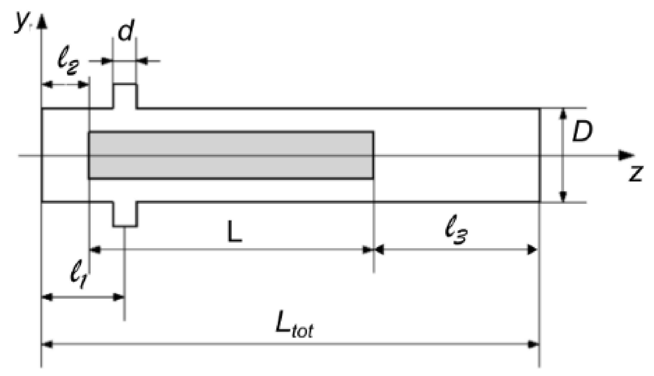
2.3. Design Parameters

Four factors, including both flow and geometrical parameters, have been considered to perform a sensitivity analysis: the pressure difference across the microgrippers $\Delta p$, the lateral hole inner diameter (d), the releasing mass length (L) and the microgrippers’ body inner diameter (D). The other geometric quantities ($l_1$ = 3.25 mm, $l_2$ = 2.1 mm, $l_3$ = 10 mm, $D_1$ = 2.6 mm) shown in Figure 5 have been kept constant. A classic full factorial DOE design was adopted and three levels were chosen for each factor. Convenient numerical values have been established for each level in accordance with the size of the device inside a region of interest, as shown in

Table 1. Factors and levels for the DOE analysis.

Main Factor	Low	Middle	High
d [mm]	0.59	0.69	0.77
L [mm]	16.2	24.2	32.2
D [mm]	3.2	3.4	3.6
Δp [kPa]	10	20	30

.

Twenty-seven geometric configurations, obtained from all possible combinations of geometric parameters’ values shown in Table 1, were tested. Each configuration was studied for the three chosen values of $\Delta p$ = 10, 20, and 30 kPa: 81 CFD simulations were performed.

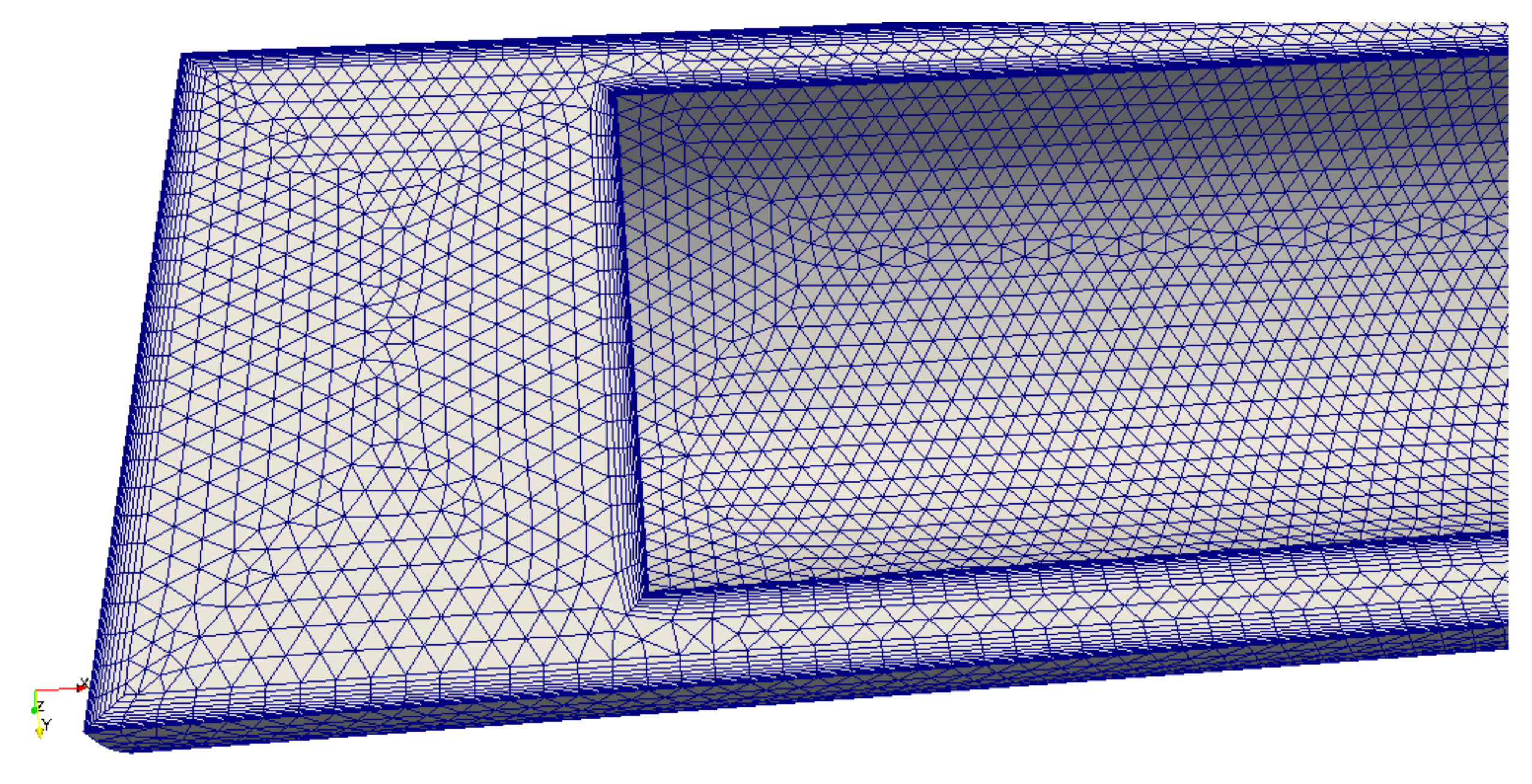
2.4. CFD Analysis

Numerical analysis of the simplified model of the gripper was performed using the open source CFD toolbox OpenFOAM [16]. The RANS approach coupled with the SST k-ω turbulence model has been used to compute the flow-field. The choice of the turbulence model was motivated by its common use in many aerodynamical applications, its robustness and its low computational cost [17]. However, recent studies demonstrated that this model leads to erroneous predictions for complicated flows with streamline curvature, sharp edges, inhomogeneties and flow separation [18,19]. This predictive discrepancy acted as a source of uncertainty in the final results of this investigation. The steady-state solver rhoSimpleFoam based on the SIMPLE algorithm was first considered, but some convergence problems suggested the use of a pseudo-transient method. The rhoPimpleFoam solver, based on the PIMPLE algorithm, was adopted eventually. The steady state solution was obtained while increasing the Courant Friedrichs–Lewy number (CFL) value, and the corresponding time step, to make the temporal derivative negligible. In particular, the minimum (and initial) CFL was set to one, and the maximum CFL was set to 50.

In addition to the residuals’ value, another criterion was defined to check the convergence of the solution. In fact, even if the residuals’ value reduced by four order of magnitude, the solution was still oscillating. An algorithm written in Python [20] was integrated into the CFD code to check at runtime for a stop condition.

The algorithm operates on successive time intervals $\Delta$$t_i$ = $2·{10}^{-3}$ s according to the following steps:

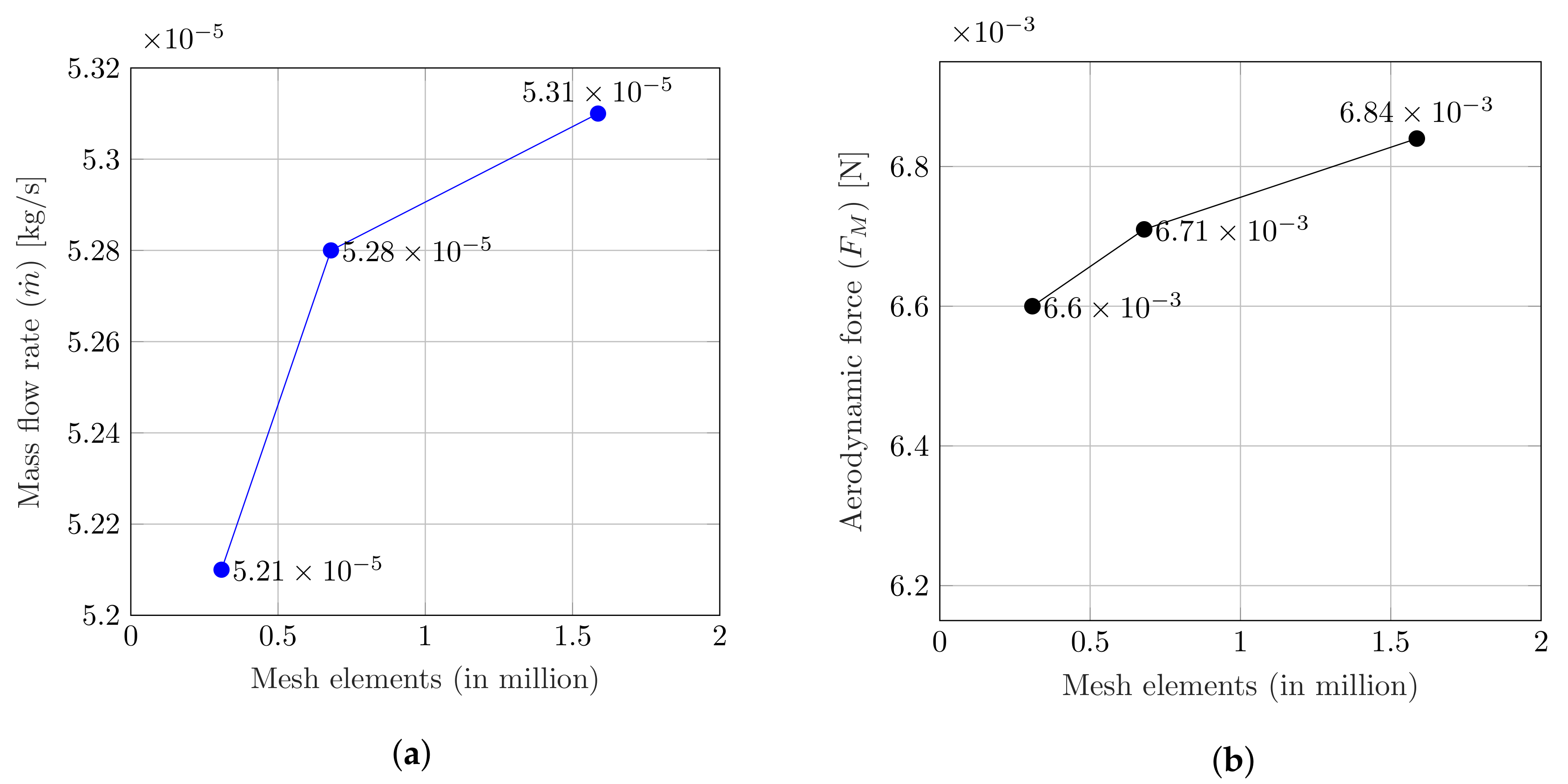
• For each i-th time interval $\Delta$$t_i$, it computes the average values of mass flow rate ($\overline{\dot{m_i}}$) and aerodynamic force ($\overline{F_{mi}}$).
• Then, it computes the levels of relative change for mass flow rate and aerodynamic force.

  $$\Delta {\dot{m}}_i=\frac{\overline{\dot{m_i}}-{\overline{\dot{m}}}_{i-1}}{{\overline{\dot{m}}}_{i-1}}$$

  (8)

  $$\Delta F_{Mi}=\frac{\overline{F_M}-{\overline{F_M}}_{i-1}}{{\overline{F_M}}_{i-1}}$$

  (9)
• It stops the simulation when both $\Delta {\dot{m}}_i$ and $\Delta F_{Mi}$ fall below a prescribed threshold (i.e., 3$·{10}^{-4}$) for the first time.

The convective terms of velocity and energy were discretized with a second-order upwind scheme, and for the diffusive terms a linear second-order bounded central scheme was used. The gradient term was evaluated using a center differencing method and the first order upwind scheme approximated the turbulent quantities.

At the inlet section, total initial temperature (T${}_{01}$ = 293.15 K), total pressure (p${}_{01}$ = 100 kPa) and turbulence intensity (Tu${}_1$ = 1%) were imposed, and static pressure (p${}_2$) was prescribed at the outlet section. The inflow velocity vector was prescribed to be normal to the inlet patch.

The mesh quality affects the accuracy of the results obtained from CFD simulations. A hybrid mesh was employed to discretize the computational domain. It consisted of prismatic elements near the walls and tetrahedra elsewhere. The near wall region, compared to a previous study [21], was extended to improve capture of the boundary layer. A non-dimensional distance y${}^{+}$≈ 1 was considered for cells near the walls, because of choice not to use the wall functions. Figure 6 shows the detail of the surface mesh in the front chamber zone.

To find out the optimal mesh density, a grid independence analysis was carried out on one gripper geometry (d = 0.77 mm, L = 24.2 mm, D = 3.4 mm), which from now on will be called “reference geometry,” using three different grid resolutions: coarse (0.308 ×${10}^6$ cells), medium (0.679 ×${10}^6$cells) and fine (1.58 ×${10}^6$ cells). The meshes were characterized by a different spacing of the elements adjacent to the walls ($y_1$) and on the model surface. However, the number of the layers ($n_L$) in the boundary layer region was modified to guarantee approximately the same boundary layer thickness ($y_{BL}$) (see

Table 2. Characteristics of grids.

Grid Density	Elements	${\mathit{y}}_1$ [mm]	${\mathit{y}}_{\mathbf{BL}}$ [mm]	${\mathit{n}}_{\mathit{L}}$
Coarse	$0.308\times {10}^6$	$1\times {10}^{-5}$	$1.64\times {10}^{-4}$	8
Medium	$0.679\times {10}^6$	$5\times {10}^{-6}$	$1.30\times {10}^{-4}$	10
Fine	$1.58\times {10}^6$	$2.5\times {10}^{-6}$	$1\times {10}^{-4}$	12

).

Figure 7a,b shows the mass flow rate ($\dot{m})$ and the aerodynamic force ($F_M$), computed using the coarse, medium and fine meshes, respectively. Small differences could be observed between medium and fine meshes for the mass flow rate, and the aerodynamic force did not show a clear grid convergence. However, the difference in the predicted force between medium and fine meshes was below 2%, which can be considered acceptable for this type of study. As a consequence, the medium mesh was used for all computations shown in the following.

3. Results

In this section, the results of the simulations are compared and discussed. In the first subsection, based on the simulations’ results, flow characteristics inside the gripper, including fluid dynamics structures, pressure and velocity distributions are analyzed. Then, trends of mass flow rate and lifting force in terms of geometrical modification are presented to investigate how geometry affects gripper performance. Eventually, empirical correlations to predict both mass flow rate and lifting force are presented in the last subsection.

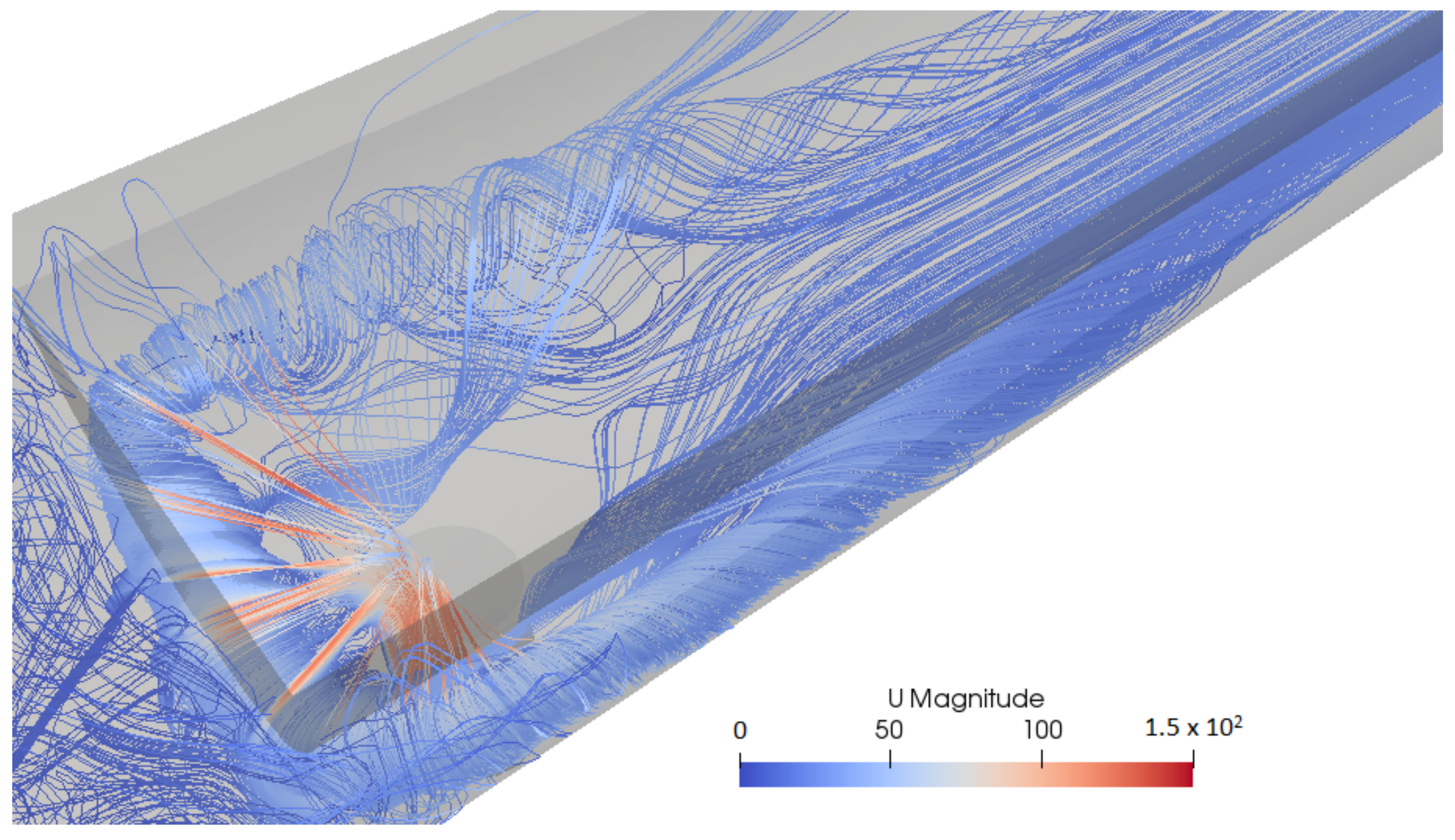
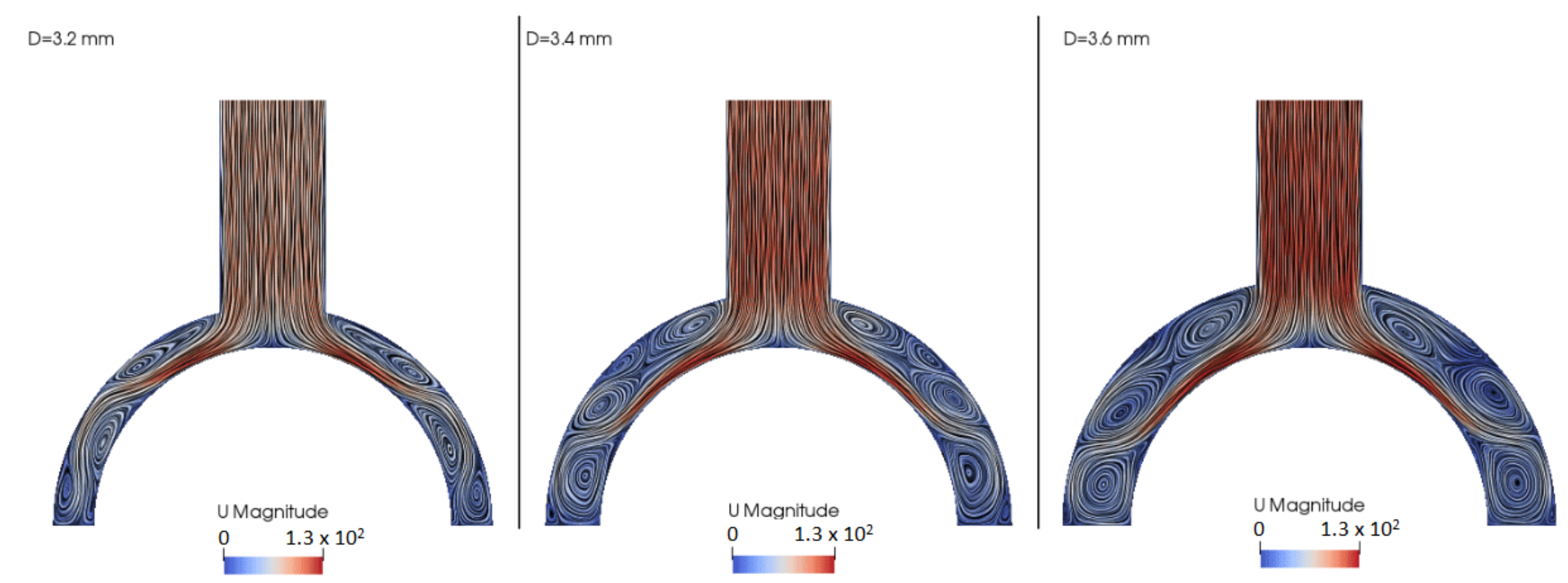
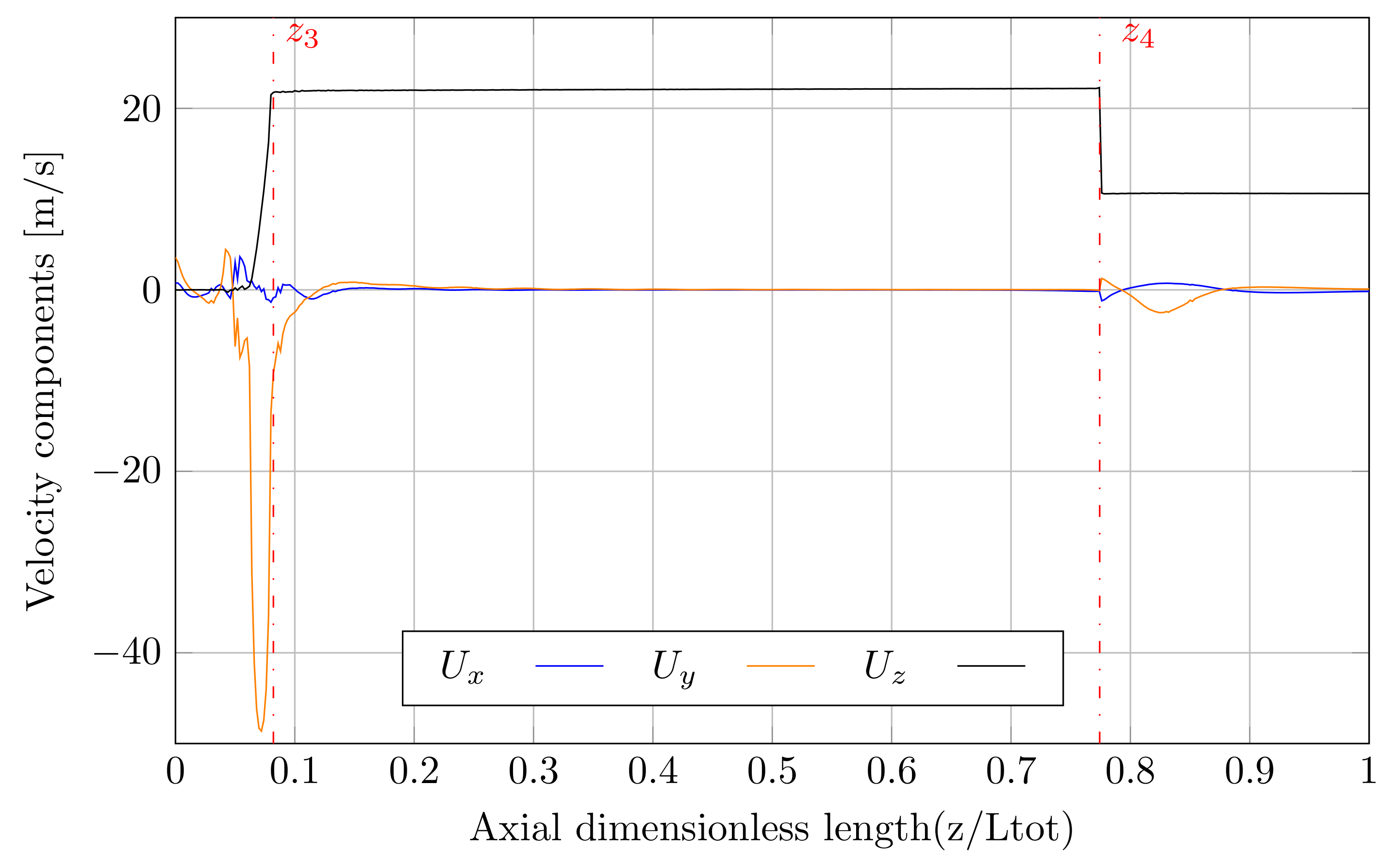
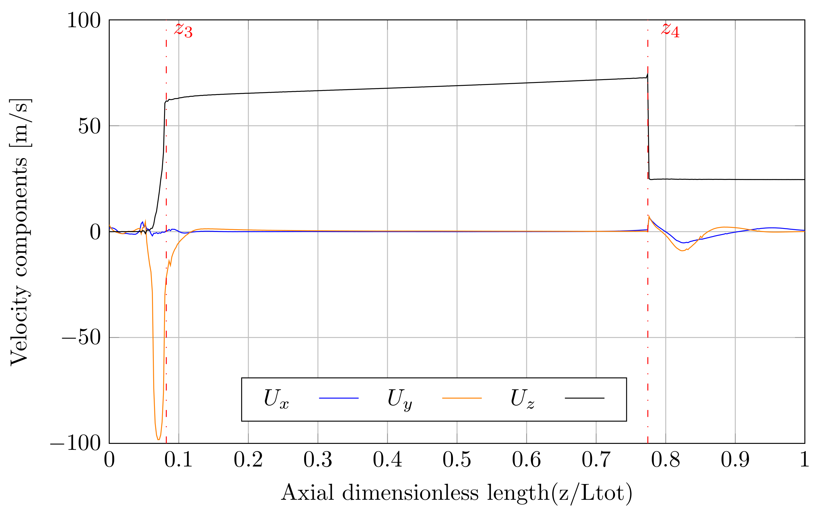
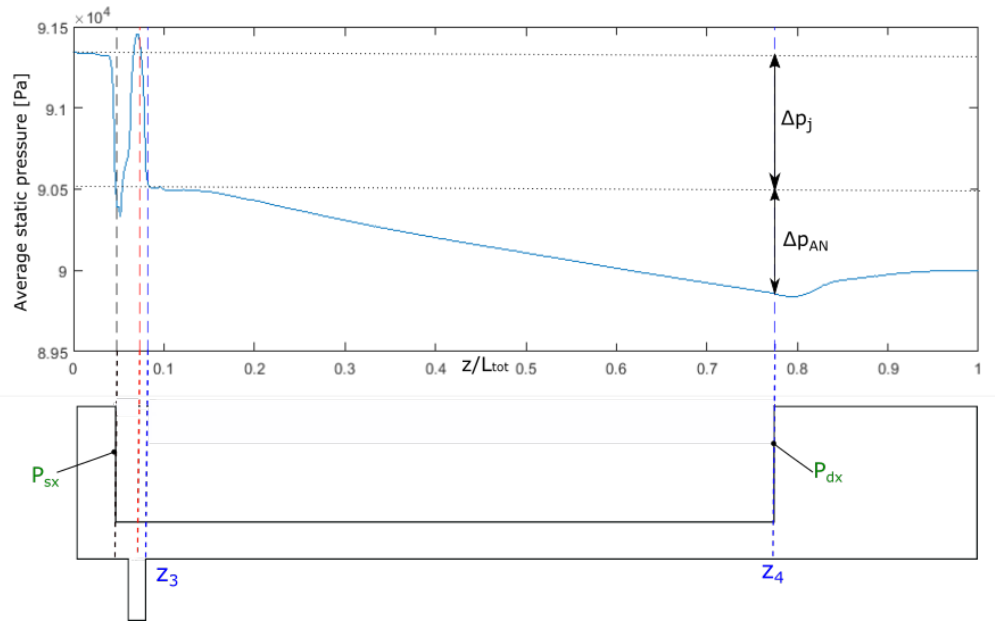
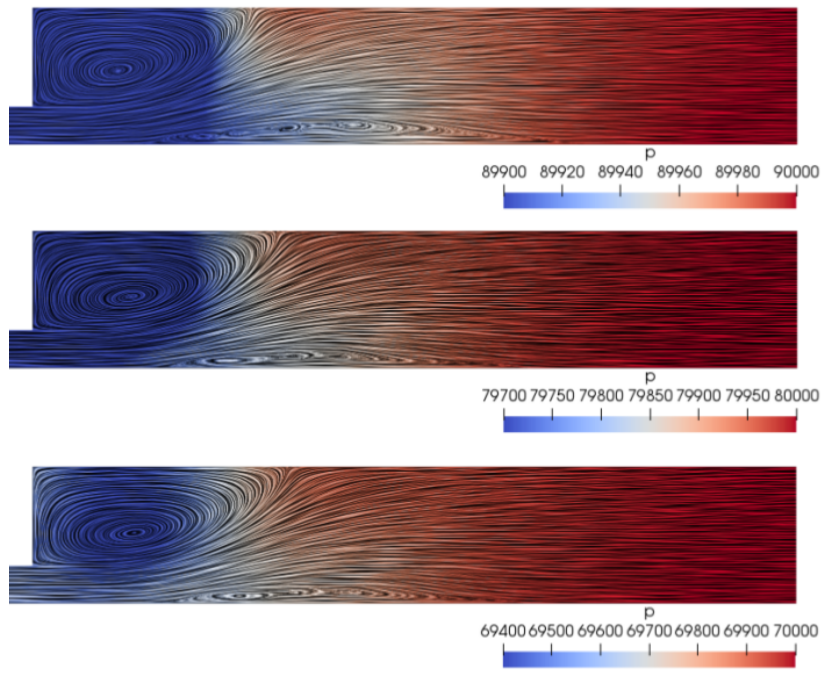
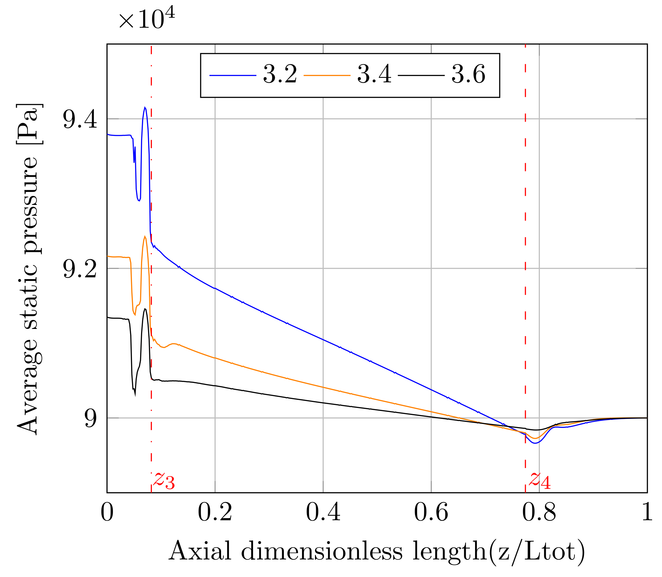
3.1. Fluid Dynamics Phenomena

Despite the simple geometry of the gripper, the flow structure that develops is rather complex due to the superposition and the interactions among several elementary flows.

Patterns reported here for the reference geometry were observed in most of the computations. For the sake of simplicity, the gripper’s inner volume was divided into four regions (front chamber, jet, annular and terminal region), as shown in Figure 8.

The airflow forced inside the gripper through the lateral hole impinges normally on the releasing mass wall, reaching a peak in static pressure (stagnation point). The jet velocity increases with the imposed negative pressure (Δp) with a maximum Mach number of 0.78 (for $\Delta p$ = 30 kPa and d = 0.77 mm): flow is subsonic in all geometrical configurations taken into account. Due to the jet impingement on the releasing mass wall, several vortical structures arise in the region nearby the lateral hole, developing along circumferential direction and tending to disappear downstream in the annular region (see Figure 9).

Figure 10 shows vortex structures development at the cross-section perpendicular to the gripper axis and passing through lateral jet axis ($z_2$) for three different gripper geometries. Vortices are symmetric with respect to the lateral jet axis, showing different shapes depending on gripper body diameter value (D). A smaller gripper body diameter indeed reduces the distance between lateral inlet and the impinging wall surface, influencing the vortices’ spatial distribution and the tendency of the flow to stay attached to the cylindrical wall. Other parameters (d, L, $p_2$) do not have such an influence on that.

Figure 11a shows the development of the average value of the static pressure, averaged over the cross-section, along the axis of the gripper. Immediately upstream of the jet, a negative pressure peak can be noted between the front chamber end ($z_1$) and the lateral jet axis ($z_2$) as a result of the vortex structure previously discussed (see Figure 11b).

The flow entering the front chamber slows down until it almost stops and the pressure stabilizes at a uniform value. In the annular region, except for the first part where the flow is still affected by the vortices associated with the jet, the transverse velocity components ($U_x$,$U_y$) tend to zero, while average average axial velocity component ($U_z$) increases and become dominant (see Figure 12). The flow accelerates in the axial direction: due to the pressure drop in the annulus, density falls sufficient quickly so that fluid velocity must rise to maintain a constant mass flow rate. The lower the outlet pressure value ($p_2$), the greater the density fall in annular region, and as a consequence, the higher the increase of velocity in axial direction (see Figure 13).

The flow at the end of the annulus region ($z_4$) detaches, creating a recirculation bubble whose length increases for lower outlet pressure. Moreover, a secondary recirculation region can be recognized close to the lateral wall due to the adverse pressure gradient occurring in the downstream region. In fact, the lowest pressure is localized just after the base of the releasing mass (see Figure 14), and a zone of diffusion is required to recover the outlet pressure. Due to the abrupt increase in the cross-sectional area, occurring while passing from the annular to the terminal region, the velocity decreases and pressure regaining occurs.

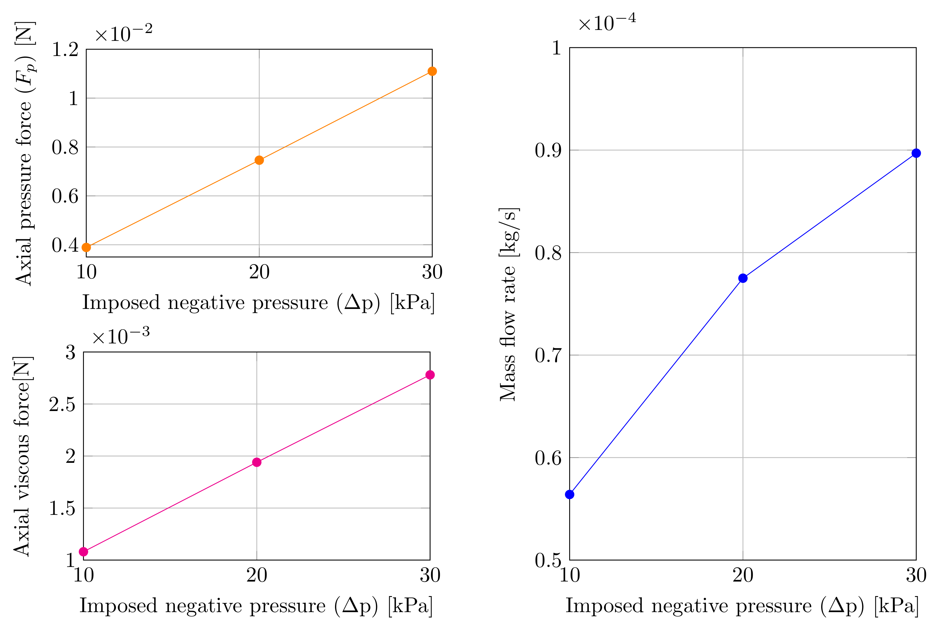
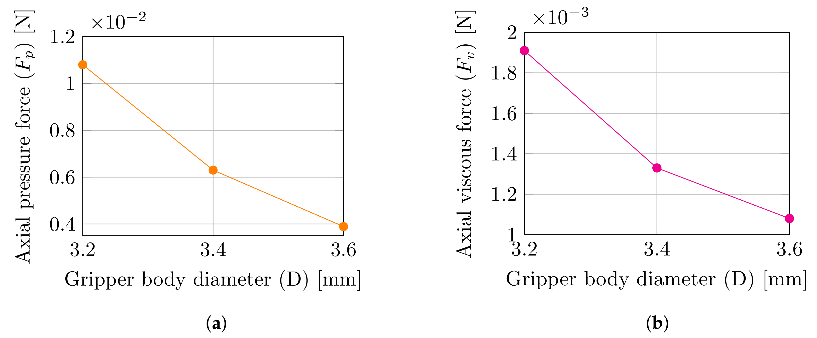
3.2. Data Analysis

The purpose of this section is to illustrate the effects of the parameters d, L, D and $p_2$ on the values of mass flow rate ($\dot{m}$) and total force on the releasing mass ($F_M$).

For a fixed geometry, decreasing outlet pressure ($p_2$) increments $\dot{m}$ and $F_M$ (see Figure 15). The incrementation of $F_M$ can be ascribed to both pressure and viscosity components. Indeed, decreasing the outlet pressure, a lower pressure is expected also at the base of the releasing mass (near the outflow). Moreover the viscous component increases due to the higher shear stress acting on the releasing mass lateral surface.

For a fixed outlet pressure, increasing the lateral hole diameter (d) provides higher mass flow rate ($\dot{m}$) and lifting force ($F_M$) on the releasing mass. The value of L slightly affects mass flow rate, while it influences the viscous part of the lifting force. It is interesting to note how the lifting force ($F_M$) is strongly related to D value (see Figure 16a,b). A larger annulus area reduces shear stress on the lateral surface, and consequentially, viscous force ($F_V$) acting on the releasing mass wall decreases.

Similarly, pressure force ($F_P$) increases as D decreases. Since the pressure force acting on the releasing mass is related to the pressure difference acting on its two bases, ($p_{sx}$ and $p_{dx}$) a possible explanation for $F_P$ trend can be found out by looking at the pressure drop in the different regions of the gripper. As can be seen from Figure 17, the pressure in the front chamber is approximately constant and equal to the pressure acting on the upstream releasing mass base ($p_{sx}$). Considering Figure 17 where average static pressure on cross-sections versus dimensionless axial direction ($z/L_{tot}$) is plotted, the pressure difference acting on the releasing mass ($p_{sx}$ – $p_{dx}$) can be written as:

$$p_{sx}-p_{dx}=\Delta p_j+\Delta p_{AN}$$

(10)

where $\Delta p_j=p_{sx}-p\left(z_3\right)$ is the pressure difference between the front chamber and the end of the jet region, and $\Delta p_{AN}$ is the pressure difference in the annular region.

The pressure drop ($\Delta p_j$ ) is controlled by the lateral impinging jet: when the distance between the releasing mass surface and the lateral inlet is smaller, as happens for smaller values of D, the distribution of the mean static pressure on the impinging surface, which typically has a Gaussian shape, exhibits higher peak pressure. As a result, higher pressure drop is expected between the front chamber and the end of the jet region. Despite the mass flow rate decreasing for decreasing D, the pressure drop in the annulus region increases, as shown in Figure 18.

This behavior can be justified as follows. Assuming that the flow in annulus can be approximated as one-dimensional (average average axial velocity $u_z$ is dominant), the momentum conservation equation reads:

$$\dot{m}d{u}_z=-A_{AN}dp-{\tau }_{w}Pdz$$

(11)

where $A_{AN}=\pi \frac{{D^2-D_1}^2}{4}$ is the cross-sectional area, $P=\pi (D+D_1)$ is the wetted perimeter and ${\tau }_w$ is the wall shear stress in the annulus region. By further rearranging Equation (11) results in:

$$\frac{dp}{dz}=-\frac{\dot{m}}{A_{AN}}\frac{d{u}_z}{dz}-\frac{4{\tau }_w}{D-D_1}$$

(12)

Since $\dot{m}=\rho u_z{A}_{AN}$ is uniform along the annulus, it holds true that

$$\rho \frac{d{u}_z}{dz}=-\frac{\dot{m}}{A_{AN}}\frac{1}{\rho }\frac{d\rho }{dz},$$

(13)

whereas the order of magnitude of the shear stress ${\tau }_w$ can be estimated as

$${\tau }_w=\mu \frac{u_z}{D-D_1}=\nu \frac{\dot{m}}{A_{AN}(D-D_1)}$$

(14)

Equation (12) can be rewritten as

$$\frac{dp}{dz}={\left(\frac{\dot{m}}{\rho A_{AN}}\right)}^2\frac{d\rho }{dz}-4\nu \frac{\dot{m}}{A_{AN}{(D-D_1)}^2}$$

(15)

Equation (15) integrated along the annular region yields the pressure drop in the annulus ($\Delta p_{AN}$):

$${\int }_{z_3}^{z_4}\frac{dp}{dz}dz$$

(16)

Since $\dot{m}$ depends almost linearly on D, as will be shown in Section 3.3 underneath, and the area of the annulus $A_{AN}$ is proportional to the square of D, the ratio $\frac{\dot{m}}{A_{AN}}$ increases as D decreases. Therefore, both terms on the right-hand side of Equation (15) increase for decreasing D.

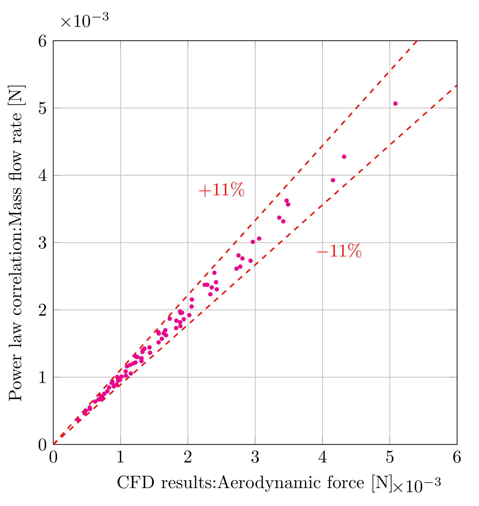
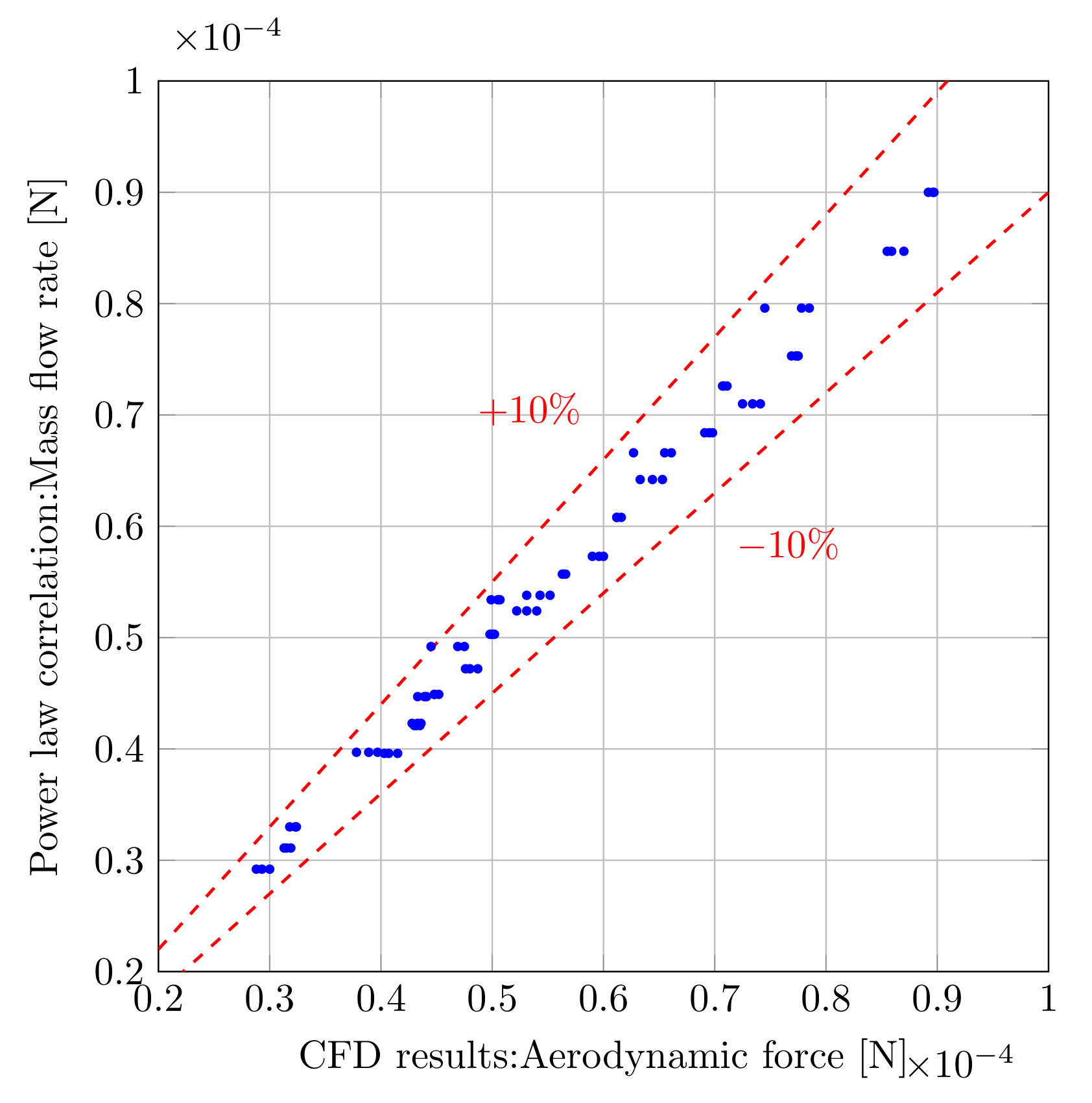
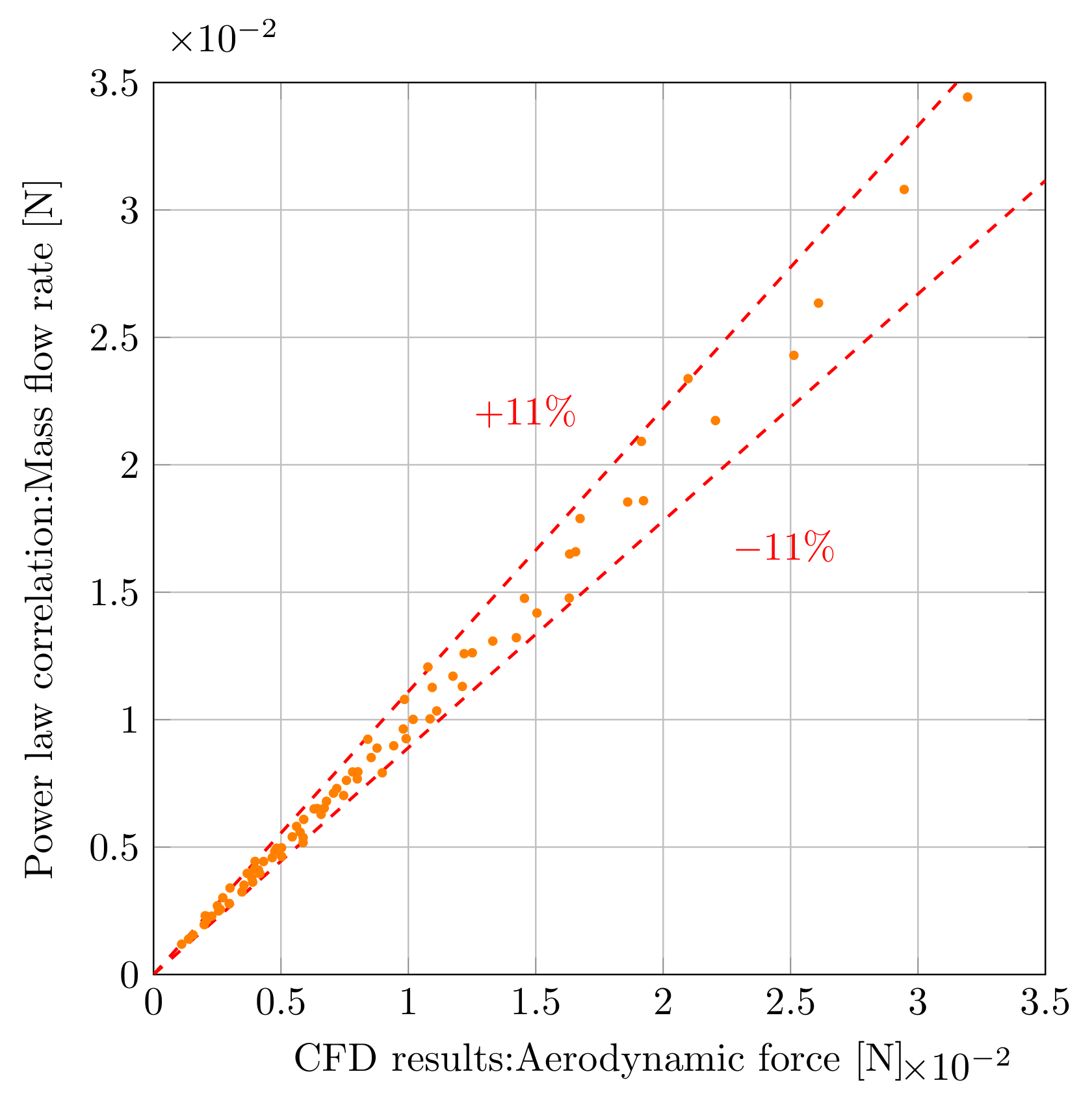
3.3. Empirical Correlations

A power law model was chosen to express the dependence of mass flow rate ($\dot{m}$), pressure force ($F_P$) and viscous force ($F_V)$ on the geometrical factors (d, L, D) and the prescribed pressure (Δp):

$$f=A\prod _j{x_j}^{\alpha j}+\epsilon$$

(17)

where f is the dependent variable we want to model (often called response), $x_j$ are the independent variables (often-called predictors), ${\alpha }_j$ are the model exponents and $ϵ$ is the model error. Even if a power law model is quite simple and cannot describe non-monotonic dependence on geometric factors and $\Delta p$, on limited ranges of variables, as the ones investigated in our study, they represent numerical data quite well. By log transforming both sides of Equation (17), it is possible to obtain a linear form (Equation (18)) that can be studied using a multiple linear regression approach.

$$\log f=\log A+\sum _j{\alpha }_j\log x_j+\log \epsilon$$

(18)

According to Equation (18), the following three power law models were assumed:

$$\log \dot{m}=a_0+a_1\log d+a_2\log L+a_3\log D+a_4\log \Delta p+\widetilde{{\epsilon }_{\dot{m}}},$$

(19)

$$\log F_P=b_0+b_1\log d+b_2\log L+b_3\log D+b_4\log \Delta p+\widetilde{{\epsilon }_{F_M}},$$

(20)

$$\log F_V=c_0+c_1\log d+c_2\log L+c_3\log D+c_4\log \Delta p+\widetilde{{\epsilon }_{F_V}},$$

(21)

Instead of searching only one correlation for the aerodynamic force $F_M$, pressure and viscous force values were modeled separately. The reason for this choice is to be found in the fact that $F_P$ and $F_V$ are related to distinct physical phenomena, and it therefore seems more appropriate to search for distinct correlations. For each response, the ordinary least square method (OLS) [22] was applied to identify the values of the model coefficients ($a_j,b_j,c_j)$ that minimize the model error ($\tilde{\epsilon }$). Moreover, significance analysis was performed to identify variables that are not statistically relevant to predicting the response. For this purpose, a statistical hypothesis test was used:

$$H_0:{\alpha }_j=0$$

(22)

The null hypothesis ($H_0$) means that the generic model coefficient ${\alpha }_j$ is equal to zero and the associated variable $x_j$ does not affect the response. However, even if a variable $x_j$ has no influence on the response (null hypothesis is true), there is a probability, expressed by the p-value, that the OLS method applied to the available sample data provides a coefficient ${\alpha }_j$ significantly higher than zero. So the smaller the p-value, the stronger the evidence that the associate variable represents a meaningful addition to the model.

A backward elimination approach [22] was employed to define the model. It starts from all potential predictors in the regression model and at each step removes the predictor with higher p-value, if greater than the chosen significance level, set to 0.05 [23].

This continues until all variables left in the model are significant.

The following empirical correlations were identified:

$$\dot{m}=9.88\times {10}^{-6}{\left(d\right)}^{1.9578}{\left(L\right)}^{-0.0141}{\left(D\right)}^{1.0428}{\left(\Delta p\right)}^{0.4371},$$

(23)

$$F_P=114.27{\left(d\right)}^{3.1780}{\left(L\right)}^{0.3896}{\left(D\right)}^{-10.21}{\left(\Delta p\right)}^{0.9545},$$

(24)

$$F_V=3.85\times {10}^{-2}{\left(d\right)}^{2.3213}{\left(L\right)}^{0.5931}{\left(D\right)}^{-5.52}{\left(\Delta p\right)}^{0.8655}.$$

(25)

Table 3. Model coefficient and significance analysis: mass flow rate.

Associated Variable	p-Value	Model Coefficients
Intercept	<2 $\times {10}^{-6}$	9.88 $\times {10}^{-6}$
d	<2 $\times {10}^{-6}$	1.9578
L	0.00454	−0.0141
D	<2 $\times {10}^{-6}$	1.0428
Δp	<2 $\times {10}^{-6}$	0.4371

,

Table 4. Model coefficient and significance analysis: pressure force.

Associated Variable	p-Value	Model Coefficients
Intercept	<2$\times {10}^{-6}$	114.2668
d	<2 $\times {10}^{-6}$	3.1780
L	<2 $\times {10}^{-6}$	0.3896
D	<2 $\times {10}^{-6}$	−10.2100
Δp	<2 $\times {10}^{-6}$	0.9545

and

Table 5. Model coefficient and significance analysis: viscous force.

Associated Variable	p-Value	Model Coefficients
Intercept	<2 $\times {10}^{-6}$	3.85 $\times {10}^{-2}$
d	<2 $\times {10}^{-6}$	2.3213
L	<2 $\times {10}^{-6}$	0.5931
D	<2 $\times {10}^{-6}$	−5.5231
Δp	< 2$\times {10}^{-6}$	0.8655

show the output of the significance analysis that has been used to define the empirical correlations.

Figure 19, Figure 20 and Figure 21 compare the mass flow rate ($\dot{m}$), the pressure force ($F_P$) and the viscous force ($F_V$), as computed in CFD simulations and the prediction empirical models. All models achieved good agreement with CFD data with an average error below 10% for the mass flow rate and 11% for force values.

4. Conclusions

In this paper, the fluid dynamics of vacuum microgrippers with an integrated releasing tool were numerically investigated. The aim was to analyze how gripper geometry and negative pressure affect the mass flow rate inside the device ($\dot{m}$) and the aerodynamic force on the releasing tool ($F_M$), which both have a key role in providing proper design of the gripper. The three empirical correlations proposed to foresee $\dot{m}$ and the two contributions of $F_M$ (i.e., pressure force $F_P$ and viscous force $F_V$) showed good agreement (average error less than 10%) with the CFD results and could represent a useful tool with which to perform preliminary design of a device to comply with the required manipulation performance.

References

- Castillo, J.; Dimaki, M.; Svendsen, W.E.; Castillo, J. Manipulation of biological samples using micro and nano techniques. Integr. Biol. 2009, 30–42. [Google Scholar] [CrossRef] [PubMed]
- Gultepe, E.; Randhawa, J.S.; Kadam, S.; Yamanaka, S.; Selaru, F.M.; Shin, E.J.; Kalloo, A.N.; Gracias, D.H. Biopsy with Thermally-Responsive Untethered Microtools. Advenced Mater. 2013, 514–519. [Google Scholar] [CrossRef] [PubMed] [Green Version]
- Monkman, G.J.; Hesse, S.; Steinmann, R.; Schunk, H. Robot Grippers; WILEY-VCH: Heppenheim, Germany, 2007. [Google Scholar]
- Nugent, G.C.; Barker, B.S.; Grandgenett, N. Robotics: Concepts methodologies tools and applications. In Impact Educ. Robot. Student STEM Learn. Attitudes, Work. Ski.; IGI Global: Hershey, PA, USA, 2014; pp. 1442–1459. [Google Scholar]
- Madou, M.J. Fundamentals of Microfabrication: The Science of Miniaturization; CRC Press: Boca Raton, FL, USA, 2018. [Google Scholar]
- Michel, F.; Ehrfeld, W. Mechatronic micro devices. In Proceedings of the 1999 International Symposium on Micromechatronics and Human Science (Cat. No. 99TH8478), Nagoya, Japan, 23–26 November 1999; pp. 27–34. [Google Scholar] [CrossRef]
- Spero, R.C.; Vicci, L.; Cribb, J.; Bober, D.; Swaminathan, V.; Brien, E.T.O.; Rogers, S.L.; Superfine, R. High throughput system for magnetic manipulation of cells , polymers , and biomaterials. Rev. Sci. Instrum. 2011, 79, 083707. [Google Scholar] [CrossRef] [PubMed] [Green Version]
- Petrovic, D.; Popovic, G.; Chatzitheodoridis, E.; Medico, O.D.; Sümecz, F.; Brenner, W.; Detter, H. Gripping Tools for Handling and Assembly of Microcomponents. In Proceedings of the 23rd International Conference on Microelectronics. Proceedings (Cat. No.02TH8595), Nis, Yugoslavia, 12–15 May 2002; Volume 1, pp. 12–15. [Google Scholar] [CrossRef]
- Zesch, W.; Brunner, M.; Weber, A. Vacuum Tool for Handling Microobjects with a Nanorobot. In Proceedings of the International Conference on Robotics and Automation, Albuquerque, NM, USA, 25 April 1997. [Google Scholar]
- Rong, W.; Fan, Z.; Wang, L.; Xie, H.; Sun, L. A vacuum microgripping tool with integrated vibration releasing capability. Rev. Sci. Instrum. 2014, 85, 085002. [Google Scholar] [CrossRef] [PubMed]
- Takahashi, K.; Kajihara, H.; Urago, M.; Saito, S.; Mochimaru, Y.; Onzawa, T. Voltage required to detach an adhered particle by Coulomb interaction for micromanipulation. J. Appl. Phys. 2003, 90, 432–437. [Google Scholar] [CrossRef]
- Ruggeri, S.; Legnani, G.; Fontana, G.; Fassi, I. Design Strategies for Vacuum Micro-Grippers With Integrated Release System. In Proceedings of the ASME 2017 International Design Engineering Technical Conferences and Computers and Information in Engineering Conference IDERC/CIE 2017, Cleveland, OH, USA, 6–9 August 2017; pp. 1–7. [Google Scholar] [CrossRef]
- Fearing, R. Survey of Sticking Effects for Micro Parts Handling. In Proceedings of the 1995 IEEE/RSJ International Conference on Intelligent Robots and Systems. Human Robot Interaction and Cooperative Robots, Pittsburgh, PA, USA, 5–9 August 1995. [Google Scholar] [CrossRef]
- Fontana, G.; Ruggeri, S.; Legnani, G.; Fassi, I. Precision handling of electronic components for PCB rework. In Proceedings of the International Precision Assembly Seminar IPAS, Chamonix, France, 16–18 February 2014; Springer: Berlin/Heidelberg, Germany, 2014; pp. 52–60. [Google Scholar] [CrossRef]
- Fontana, G.; Ruggeri, S.; Ghidoni, A.; Morelli, A.; Legnani, G.; Lezzi, A.M.; Fassi, I. Fluid Dynamics Aided Design of an Innovative Micro-Gripper. In Proceedings of the International Precision Assembly Seminar IPAS, Chamonix, France, 14–16 January 2018; Springer International Publishing: Berlin/Heidelberg, Germany, 2019; Volume 1, pp. 214–225. [Google Scholar] [CrossRef] [Green Version]
- OpenFOAM 4.1. Available online: https://openfoam.org (accessed on 13 October 2016).
- Menter, F.R. Two-equation eddy-viscosity turbulence models for engineering applications. AIAA J. 1994, 32, 1598–1605. [Google Scholar] [CrossRef] [Green Version]
- Mishra, A.A.; Mukhopadhaya, J.; Iaccarino, G.; Alonso, J. Uncertainty estimation module for turbulence model predictions in SU2. AIAA J. 2019, 57, 1066–1077. [Google Scholar] [CrossRef]
- Heyse, J.F.; Mishra, A.A.; Iaccarino, G. Estimating RANS model uncertainty using machine learning. J. Glob. Power Propuls. Society. Spec. Issue Data Driven Model. High-Fidel. Simul. 2021, 1–14. [Google Scholar] [CrossRef]
- Python Language Reference, Version 3.0. Available online: http://www.python.org (accessed on 8 March 2020).
- Urbano, D.G.; Noventa, G.; Fontana, G.; Fassi, I.; Legnani, G.; Ghidoni, A.; Lezzi, A.M. CFD Analysis of an innovative vacuum micro-gripper. In Proceedings of the International Conference of Heat Transfer Fluid Mechanics and Thermodynamics, Wicklow, Ireland, 22–24 July 2019. [Google Scholar]
- Draper, N.R.; Smith, H. Applied Regression Analysis; John Wiley & Sons: Hoboken, NJ, USA, 1998; Volume 326. [Google Scholar]
- Kim, J.A.E.H.; Choi, I.N. Choosing the Level of Significance: A Decision-theoretic Approach. ABACUS 2019, 1–45. [Google Scholar] [CrossRef]