On the Reversible Jump Markov Chain Monte Carlo (RJMCMC) Algorithm for Extreme Value Mixture Distribution as a Location-Scale Transformation of the Weibull Distribution

Abstract

Data with a multimodal pattern can be analyzed using a mixture model. In a mixture model, the most important step is the determination of the number of mixture components, because finding the correct number of mixture components will reduce the error of the resulting model. In a Bayesian analysis, one method that can be used to determine the number of mixture components is the reversible jump Markov chain Monte Carlo (RJMCMC). The RJMCMC is used for distributions that have location and scale parameters or location-scale distribution, such as the Gaussian distribution family. In this research, we added an important step before beginning to use the RJMCMC method, namely the modification of the analyzed distribution into location-scale distribution. We called this the non-Gaussian RJMCMC (NG-RJMCMC) algorithm. The following steps are the same as for the RJMCMC. In this study, we applied it to the Weibull distribution. This will help many researchers in the field of survival analysis since most of the survival time distribution is Weibull. We transformed the Weibull distribution into a location-scale distribution, which is the extreme value (EV) type 1 (Gumbel-type for minima) distribution. Thus, for the mixture analysis, we call this EV-I mixture distribution. Based on the simulation results, we can conclude that the accuracy level is at minimum 95%. We also applied the EV-I mixture distribution and compared it with the Gaussian mixture distribution for enzyme, acidity, and galaxy datasets. Based on the Kullback–Leibler divergence (KLD) and visual observation, the EV-I mixture distribution has higher coverage than the Gaussian mixture distribution. We also applied it to our dengue hemorrhagic fever (DHF) data from eastern Surabaya, East Java, Indonesia. The estimation results show that the number of mixture components in the data is four; we also obtained the estimation results of the other parameters and labels for each observation. Based on the Kullback–Leibler divergence (KLD) and visual observation, for our data, the EV-I mixture distribution offers better coverage than the Gaussian mixture distribution.

1. Introduction

Understanding the type of distribution of data is the first step in a data-driven statistical analysis, especially in a Bayesian analysis. This is very important because the distribution that we use must be as great as possible to cover the data we have. By knowing the distribution of the data, the error in the model can be minimized. However, it is not rare for the identified data to have a multimodal pattern. A model with data that has a multimodal pattern becomes imprecise when it is analyzed using a single mode distribution. This type of data is best modeled using mixture analysis. The most important thing in the mixture analysis is to determine the number of mixture components. If we know the correct number of mixture components, then the error in the resulting model can be minimized. In this way, our model will describe the real situation, because it is data-driven.

There are several methods for determining the number of mixture components in a dataset. Roeder [1] used a graphical technique to determine the number of mixture components in the Gaussian distribution. The Expectation-Maximization (EM) method was carried out by Carreira-Perpinán and Williams [2], while the Greedy EM method was carried out by Vlassis and Likas [3]. The likelihood ratio test (LRT) method has been carried out by Jeffries, Lo et al., and Kasahara and Shimotsu [4,5,6]. The LRT method was also carried out by McLachlan [7], but to the assessment null distribution, a bootstrapping approach was employed. A comparison between EM and LRT methods to determine the number of mixture components was carried out by Soromenho [8]. The determination of the number of mixture components using the inverse-Fisher information matrix was carried out by Bozdogan [9], and modification of the information matrix was carried out by Polymenis and Titterington [10]. Baudry et al. [11] used the Bayesian information criterion (BIC) method for clustering. In a comparison of several methods carried out by Lukočiene and Vermunt [12], these methods are the Akaike information criterion (AIC), BIC, AIC3, consistent AIC (CAIC), the information theoretic measure of complexity (ICOMP), and log-likelihood. Miller and Harrison [13] and Fearnhead [14] used the Dirichlet mixture process (DPM). Research conducted by McLachlan and Rathnayake [15] investigated several methods, including the LRT, resampling, information matrix, Clest method, and BIC methods. The methods mentioned above are used in the Gaussian distribution.

For complex computations, there is a method from the Bayesian perspective to determine the number of mixture components of the distribution, namely the reversible jump Markov chain Monte Carlo (RJMCMC). This method was initially introduced by Richardson and Green [16]. They used this method to determine the number of mixture components in the Gaussian distribution. This method is very flexible since it allows one to identify the number of components in data with a known or unknown number of components [17]. RJMCMC is also able to move between subspace parameters depending on the model, though the number of mixture components is different. Mathematically, the RJMCMC is simply derived in its random scan form; when the available moves are scanned systematically, the RJMCMC will be as valid as the idea from Metropolis-Hastings methods [18]. In real life, the RJMCMC can be applied to highly dimensional data [19]. Several studies have used the RJMCMC method for the Gaussian distribution [17,18,20,21,22,23,24,25,26,27,28].

Based on the advantages of the RJMCMC method as well as the previous studies mentioned above, this method will be powerful if it can be used not only in the Gaussian mixture distribution, because the Gaussian mixture is certainly not always the best approximation in some cases, although it may provide a reasonable approximation to many real-word distribution situations [29]. For example, if this method can be used on data with a domain more than zero, this would be very helpful to researchers in the fields of survival, reliability, etc. In most cases, survival data follow the Weibull distribution. Several studies of survival data using the Weibull distribution have been conducted [30,31,32,33,34,35,36,37]. Studies using the Weibull distribution for reliability were carried out by Villa-Covarrubias et al. and Zamora-Antuñano et al. [38,39]. In addition, some studies used Weibull mixture distribution for survival data [40,41,42,43,44,45,46,47,48,49,50,51]. According to the above studies that used the Weibull mixture distribution, the determination of the number of mixture components is a consideration. Determining the number of mixture components is an important first step in the mixture model. Therefore, we created a new algorithm that is a modification of the RJMCMC method for non-Gaussian distributions; we called it the non-Gaussian RJMCMC (NG-RJMCMC) algorithm. What we have done is to convert the original distribution of the data into a location-scale distribution, so that it has the same parameters as the Gaussian distribution, and finally the RJMCMC method can be applied. Thus, the number of mixture components can be determined before further analysis. In particular, our algorithm can help researchers in the field of survival by utilizing the Weibull mixture distribution. In general, our algorithm can be applied to any mixture distribution, converting the original distribution into a location-scale family.

Several studies using the RJMCMC method on the Weibull distribution have been carried out. First, Newcombe et al. [52] used the RJMCMC method to implement a Bayesian variable selection for the Weibull regression model for breast cancer survival cases. The study conducted by Denis and Molinari [53] also used the RJMCMC method as covariate selection for the Weibull distribution in two datasets, namely Stanford heart transplant and lung cancer survival data. Mallet et al. [54] used the RJMCMC method to search for the best configuration of functions for Lidar waveforms. In their library of modeling functions, there are generalized Gaussian, Weibull, Nakagami, and Burr distributions. With their analysis, the Lidar waveform is a combination of these distributions. In our research, we have used the RJMCMC method on the Weibull distribution but from a different perspective, namely identifying multimodal data by determining the number of components, then determining the membership of each mixture component and determining the estimation results.

This paper is organized as follows. Section 2 introduces the basic formulation for the Bayesian mixture model and hierarchical model in general. Section 3 describes the location-scale distributions and NG-RJMCMC algorithm. Section 4 describes the transformation from the Weibull distribution to the location-scale distribution, determining the prior distributions, and explaining the move types in the RJMCMC method. Section 5 contains the simulation study. Section 6 provides misspecification cases as the opposite of a simulation study to strengthen the proposed method. Section 7 provides analysis results for applications of enzyme, acidity, and galaxy datasets, as well as our data, namely dengue hemorrhagic fever (DBD) in eastern Surabaya, East Java, Indonesia. The conclusions are given in Section 8.

2. Bayesian Model for Mixtures

2.1. Basic Formulation

For independent scalar or vector observations $t_i$, the basic mixture model can be written as in Equation (1):

$$t_i\sim {\displaystyle \sum _{j=1}^k{w}_j}f\left(\cdot |{\theta }_j\right)\hspace{1em}\mathrm{independently}\mathrm{for}i=1,2,\cdots ,n,$$

(1)

where $f\left(\cdot |\theta \right)$ is a given parametric family of densities indexed by a scalar or vector parameter $\theta$ [16]. The purpose of this analysis is to infer to the unknown: the number of components ($k$), the weights of components ($w_j$), and the parameters of components (${\theta }_j$). Suppose a heterogeneous population consists of groups $j=1,2,\cdots ,k$ in proportion to $w_j$. The identity or label of the group is unknown for every observation. In this context, it is natural to create a group label $z_i$ for the $i$-th observation as a latent allocation variable. The unobserved vector $z=\left(z_1,z_2,\cdots ,z_n\right)$ is usually known as the “membership vector” of the mixture model [29]. Then, $z_i$ is assumed to be drawn independently of the distributions

$$\mathrm{Pr}\left(z_i=j\right)=w_j\hspace{1em}\hspace{1em}\hspace{1em}\hspace{1em}\hspace{1em}\mathrm{for}j=1,2,\cdots ,k.$$

(2)

2.2. Hierarchical Model in General

As explained in the previous subsection, there are three unknown components, $k$, $w$, and $\theta$. In the Bayesian framework, these three components are drawn from the appropriate prior distribution [16]. The joint distribution of all variables can be written as in Equation (3):

$$\mathrm{Pr}\left(k,w,z,\theta ,t\right)=\mathrm{Pr}\left(k\right)\mathrm{Pr}\left(w|k\right)\mathrm{Pr}\left(z|w,k\right)\mathrm{Pr}\left(\theta |z,w,k\right)\mathrm{Pr}\left(t|\theta ,z,w,k\right),$$

(3)

where $w={\left(w_j\right)}_{j=1,2,\cdots ,k}$, $z={\left(z_i\right)}_{i=1,2,\cdots ,n}$, $\theta ={\left({\theta }_j\right)}_{j=1,2,\cdots ,k}$, $t={\left(t_i\right)}_{i=1,2,\cdots ,n}$, and $\mathrm{Pr}\left(\cdot |\cdot \right)$ are the generic conditional distributions [16]. Then, Equation (3) may be forced naturally, so that $\mathrm{Pr}\left(\theta |z,w,k\right)=\mathrm{Pr}\left(\theta |k\right)$ and $\mathrm{Pr}\left(t|\theta ,z,w,k\right)=\mathrm{Pr}\left(t|\theta ,z\right)$ [16]. Therefore, for the Bayesian hierarchical model, the joint distribution in Equation (3) can be simplified into Equation (4):

$$\mathrm{Pr}\left(k,w,z,\theta ,t\right)=\mathrm{Pr}\left(k\right)\mathrm{Pr}\left(w|k\right)\mathrm{Pr}\left(z|w,k\right)\mathrm{Pr}\left(\theta |k\right)\mathrm{Pr}\left(t|\theta ,z\right).$$

(4)

Next, we add an additional layer to the hierarchy, namely hyperparameters $\gamma$, $\delta$, and $\xi$ for $k$, $w$, and $\theta$, respectively. These hyperparameters will be drawn from independent hyperpriors. The joint distribution of all variables is then given in Equation (5):

$$\mathrm{Pr}\left(\gamma ,\delta ,\xi ,k,w,z,\theta ,t\right)=\mathrm{Pr}\left(\gamma \right)\mathrm{Pr}\left(\delta \right)\mathrm{Pr}\left(\xi \right)\mathrm{Pr}\left(k|\gamma \right)\mathrm{Pr}\left(w|k,\delta \right)\mathrm{Pr}\left(z|w,k\right)\mathrm{Pr}\left(\theta |k,\xi \right)\mathrm{Pr}\left(t|\theta ,z\right)$$

(5)

3. Non-Gaussian Reversible Jump Markov Chain Monte Carlo (NG-RJMCMC) Algorithm for Mixture Model

3.1. The Family of Location-Scale Distributions

A random variable $T$ is defined as belonging to the location-scale family when its cumulative distribution function (CDF)

$$F_T\left(t|\mu ,\sigma \right)=\mathrm{Pr}\left(T\le t|\mu ,\sigma \right)$$

is a function only of $\frac{t-\mu }{\sigma }$, as in Equation (6) [55]:

$$F_T\left(t|\mu ,\sigma \right)=F\left(\frac{t-\mu }{\sigma }\right);\mu \in ℝ,\sigma >0,$$

(6)

where $F(\cdot )$ is a distribution without other parameters. The two-dimensional parameter ($\mu ,\sigma$) is called the location-scale parameter, with $\mu$ being the location parameter and $\sigma$ being the scale parameter. For fixed $\sigma =1$, we have a subfamily that is a location family with a parameter $\mu$, and for fixed $\mu =0$, we have a scale family with a parameter $\sigma$. If $T$ is continuous with the probability density function (p.d.f.)

$$f_T\left(t|\mu ,\sigma \right)=\frac{d{F}_T\left(t|\mu ,\sigma \right)}{dt}$$

then ($\mu ,\sigma$) is a location-scale parameter for $T$ if (and only if)

$$f_T\left(t|\mu ,\sigma \right)=\frac{1}{\sigma }g\left(\frac{t-\mu }{\sigma }\right),$$

(7)

where the functional form $g$ is completely specified, but the location and scale parameters, $\mu$ and $\sigma$, of $f_T\left(t|\mu ,\sigma \right)$ are unknown, and $g(\cdot )$ is the standard form of the density $f_T\left(t|\mu ,\sigma \right)$ [56,57].

3.2. NG-RJMCMC Algorithm

In the mixture model analysis, one method is known, namely the reversible jump Markov chain Monte Carlo (RJMCMC). The RJMCMC method can be used to estimate an unknown quantity, such as the number of mixture components, the weights of mixture components, and the distribution parameters of mixture components. For its usefulness in determining the number of mixture components in the indicated multimodal data, RJMCMC has been extensively used. For the Gaussian distribution, this was initially carried out by Richardson and Green [16]. Over time, RJMCMC can be used for distributions other than Gaussian. RJMCMC for general beta distribution was carried out in two studies by Bouguila and Elguebaly [29,58]. In their research, the general beta distribution consists of four parameters, namely the lower limit, the upper limit, and two shape parameters. Then, to use the RJMCMC algorithm, they obtained the location-scale parameterization for this distribution. Another study followed the location-scale parameterization for the RJMCMC method, namely research on the symmetry gamma distribution [59].

Not only in the RJMCMC method but also in other methods, the location-scale parameterization is carried out in the mixture analysis. First, research on the exponential and Gaussian distribution using the Dirichlet process mixture was carried out by Jo et al. [60]. Secondly, research on the asymmetric Laplace error distribution using the likelihood-based approach was carried out by Kobayashi and Kozumi [61]. Finally, research on the exponential distribution using the Gibbs sampler was carried out by Gruet et al. [62]. Based on the studies mentioned above, in the mixture analysis using any method, it will be easier if the distribution used in the research follows the location-scale (family) parameterization. Thus, we given Algorithm 1 as a modification of the RJMCMC algorithm.

Algorithm 1. NG-RJMCMC Algorithm

Modify the distribution to be analyzed into a member of the location-scale family, determine: (a) form of transformation, and (b) location-scale parameter Determine the appropriate priors for: (a) component weights ($w$), (b) location-scale parameter ($\mu ,\sigma$), and (c) latent allocation variable ($z$) Do all six types of RJMCMC moves by Richardson and Green [16]. A sweep is defined as a complete run on these six moves [16]: (a) updating the component weights ($w$), (b) updating the location-scale parameter ($\mu ,\sigma$), (c) updating the latent allocation variable ($z$), (d) updating the hyperparameters ($\gamma$, $\delta$, and $\xi$). Moves (a), (b), (c), and (d) can therefore be performed in parallel (e) do the splitting or combining mixture component (f) do the birth or death of an empty component.

Letting $\Delta$ denote the state variable (in this study, $\Delta$ be the complete set of unknowns ($\mu$, $\sigma$, $k$, $w$, $z$)), and $p(\Delta )$ be the target probability measure (the posterior distribution), we consider a countable family of move types, indexed by $m=1,2,\cdots$. When the current state is $\Delta$, a move type $m$ and destination ${\Delta }^{\ast }$ are proposed, with joint distribution given by $q_m\left(\Delta ,{\Delta }^{\ast }\right)$. The move is accepted with probability

$${\alpha }_m\left(\Delta ,{\Delta }^{\ast }\right)=\min \left\{1,\frac{p\left({\Delta }^{\ast }\right)q_m\left({\Delta }^{\ast },\Delta \right)}{p(\Delta )q_m\left(\Delta ,{\Delta }^{\ast }\right)}\right\}.$$

(8)

If ${\Delta }^{\ast }$ has a higher dimensional space than $\Delta$, it is possible to create a vector of continuous random variables $u$, independent of $\Delta$ [16]. Then, the new state ${\Delta }^{\ast }$ is set by an invertible deterministic function of $\Delta$ and $u$: $f\left(\Delta ,u\right)$. Then, the acceptance probability in Equation (8) can be rewritten as in Equation (9):

$${\alpha }_m\left(\Delta ,{\Delta }^{\ast }\right)=\min \left\{1,\frac{p\left({\Delta }^{\ast }\right)r_m\left({\Delta }^{\ast }\right)}{p(\Delta )r_m(\Delta )q\left(u\right)}\left|\frac{\partial {\Delta }^{\ast }}{\partial \left(\Delta ,u\right)}\right|\right\},$$

(9)

where $r_m(\Delta )$ is the probability of choosing move type $m$ when in the state $\Delta$, and $q\left(u\right)$ is the p.d.f. of $u$. The last term, $\left|\frac{\partial {\Delta }^{\ast }}{\partial \left(\Delta ,u\right)}\right|$, is the determinant of Jacobian matrix resulting from modifying the variable from $\left(\Delta ,u\right)$ to ${\Delta }^{\ast }$.

4. Bayesian Analysis of Weibull Mixture Distribution Using NG-RJMCMC Algorithm

4.1. Change the Weibull Distribution into a Member of the Location-Scale Family

4.1.1. Form of Transformation and Location-Scale Parameter of Weibull Distribution

If the random variable $T$ follows the Weibull distribution with the shape parameter $\eta >0$ and the scale parameter $\lambda >0$, $T\sim \mathrm{Weibull}\left(\eta ,\lambda \right)$, then the p.d.f. is given by Equation (10) [63]:

$$f_T\left(t|\eta ,\lambda \right)=\{\begin{array}{ll}\frac{\eta }{\lambda }{\left(\frac{t}{\lambda }\right)}^{\eta -1}{e}^{-{\left(\frac{t}{\lambda }\right)}^{\eta }}& ,t\ge 0\\ 0& ,t<0\end{array}$$

(10)

and CDF is given by Equation (11) [64]:

$$F_T\left(t|\eta ,\lambda \right)=\{\begin{array}{ll}1-e^{-{\left(\frac{t}{\lambda }\right)}^{\eta }}& ,t\ge 0\\ 0& ,t<0.\end{array}$$

(11)

Equation (11) can be rewritten as Equation (12):

$$\begin{array}{lll}{F}_T\left(t|\eta ,\lambda \right)& =& \{\begin{array}{ll}1-e^{-{\left(\frac{t-0}{\lambda }\right)}^{\eta }}& ,t\ge 0\\ 0& ,t<0\end{array}\\ & =& F_T{\left(\frac{t-\mu }{\lambda }\right)}_{\mu =0}.\end{array}$$

(12)

Based on Equation (12) and the explanation in Section 3.1, it can be concluded that the Weibull distribution is a member of the scale family. To facilitate the analysis of the Weibull distribution, it is necessary to transform it into a location-scale distribution.

If the random variable $T$ is transformed into a new variable, $Y=\ln T$, then $Y$ has an extreme value (EV) type 1 (Gumbel-type for minima) distribution with the location parameter $\mu =\ln \lambda$ and the scale parameter $\sigma =\frac{1}{\eta }$ [64,65] (this explanation can be seen in Appendix A). Therefore, the p.d.f. and CDF for $Y~\mathrm{EV}-\mathrm{I}\left(\mu =\ln \lambda ,\sigma =\frac{1}{\eta }\right)$ are given by Equations (13) and (14), respectively [56,66,67]:

$$f_Y\left(y|\mu ,\sigma \right)=\frac{1}{\sigma }\exp \left[\left(\frac{y-\mu }{\sigma }\right)-\exp \left(\frac{y-\mu }{\sigma }\right)\right]$$

(13)

$$F_Y\left(y|\mu ,\sigma \right)=1-\exp \left[-\exp \left(\frac{y-\mu }{\sigma }\right)\right],$$

(14)

where $-\infty <y<\infty$, $-\infty <\mu <\infty$, and $0<\sigma <\infty$.

4.1.2. Finite EV-I Mixture Distribution

Based on the explanation provided in the previous subsection, $T\sim \mathrm{Weibull}\left(\eta ,\lambda \right)$ as a member-scale family can be transformed into a member of the location-scale family $Y~\mathrm{EV}-\mathrm{I}\left(\mu =\ln \lambda ,\sigma =\frac{1}{\eta }\right)$, where $Y=\ln T$. It is well-known that $T\sim \mathrm{Weibull}\left(\eta ,\lambda \right)$ and $Y~\mathrm{EV}-\mathrm{I}\left(\mu =\ln \lambda ,\sigma =\frac{1}{\eta }\right)$ are equivalent models [68]. As $Y~\mathrm{EV}-\mathrm{I}\left(\mu =\ln \lambda ,\sigma =\frac{1}{\eta }\right)$ belongs to the location-scale family, it is sometimes easier to work with $Y~\mathrm{EV}-\mathrm{I}\left(\mu =\ln \lambda ,\sigma =\frac{1}{\eta }\right)$ rather than $T\sim \mathrm{Weibull}\left(\eta ,\lambda \right)$ [68], especially in the analysis of the mixture model. Consequently, the next analysis will use the variable $Y$. The EV-I mixture distribution with $k$ components is defined as in Equation (15):

$$f\left(y|\Theta \right)={\displaystyle \sum _{j=1}^k{w}_j}f\left(y|{\mu }_j,{\sigma }_j\right),$$

(15)

where $\Theta =\left(\theta ,w\right)$ refers to the complete set of parameters to be estimated, where $\theta =\left({\mu }_1,{\sigma }_1;{\mu }_2,{\sigma }_2;\cdots ;{\mu }_k,{\sigma }_k\right)$.

4.2. Determine the Appropriate Priors

4.2.1. Hierarchical Model

According to the general form of the hierarchical model in Section 2.2, a hierarchical model for the EV-I mixture distribution can be written as in Equation (16):

$$\mathrm{Pr}\left(\gamma ,\delta ,\xi ,k,w,z,\theta ,y\right)=\mathrm{Pr}\left(\gamma \right)\mathrm{Pr}\left(\delta \right)\mathrm{Pr}\left(\xi \right)\mathrm{Pr}\left(k|\gamma \right)\mathrm{Pr}\left(w|k,\delta \right)\mathrm{Pr}\left(z|w,k\right)\mathrm{Pr}\left(\theta |k,\xi \right)\mathrm{Pr}\left(y|\theta ,z\right),$$

(16)

where $k$ is the number of components, $w={\left(w_j\right)}_{j=1,2,\cdots ,k}$ is the weights of the components, $z={\left(z_i\right)}_{i=1,2,\cdots ,n}$ is the latent allocation variable, $\theta =\left({\theta }_j\right)={\left({\mu }_j,{\sigma }_j\right)}_{j=1,2,\cdots ,k}$ is the location-scale parameter, $y={\left(y_i\right)}_{i=1,2,\cdots ,n}$ is the data with $Y~\mathrm{EV}-\mathrm{I}\left(\mu ,\sigma \right)$, and $\gamma$, $\delta$, and $\xi$ are the hyperparameters for $k$, $w$, and $\theta$, respectively. If we condition on $z$, the distribution of $y_i$ is given by the $z_i$-th component in the mixture, so that $\mathrm{Pr}\left(y|\theta ,z\right)={\displaystyle \prod _{i=1}^n\mathrm{Pr}\left(y_i|{\theta }_{z_i}\right)}$ [29]. Then, the final form of the joint distribution can be found via Equation (17):

$$\mathrm{Pr}\left(\gamma ,\delta ,\xi ,k,w,z,\theta ,y\right)=\mathrm{Pr}\left(\gamma \right)\mathrm{Pr}\left(\delta \right)\mathrm{Pr}\left(\xi \right)\mathrm{Pr}\left(k|\gamma \right)\mathrm{Pr}\left(w|k,\delta \right)\mathrm{Pr}\left(z|w,k\right)\mathrm{Pr}\left(\theta |k,\xi \right){\displaystyle \prod _{i=1}^n\mathrm{Pr}\left(y_i|{\theta }_{z_i}\right)}.$$

(17)

4.2.2. Priors and Posteriors

In this section, we define the priors. In the hierarchical model in Equation (16), for each parameter, we assume that the priors are drawn independently. Based on research conducted by Yoon et al. [69], Coles and Tawn [70] and Tancredi et al. [71], the priors for the location and scale parameters in the extreme value distribution are flat. In research by Yoon et al. [69], they chose the adoption of near-flat priors for the location and scale parameters. In research by Coles and Tawn [70], the location and scale parameter priors are almost noninformative: the prior for $\mu$ is extremely flat, while that for $\sigma$ resembles $\frac{1}{\sigma }$. Based on research by Tancredi et al. [71], they have chosen a uniform distribution for the location and scale parameters. Therefore, in this study, the Gaussian distribution (with the large variance) with mean $\epsilon$ and variance ${\zeta }^2$ was selected as a prior for location parameter $\mu$. Thus, ${\mu }_j$ for each component is given by

$$f\left({\mu }_j|\epsilon ,{\zeta }^2\right)=\frac{1}{\sqrt{2\pi {\zeta }^2}}\exp \left\{-\frac{1}{2}{\left(\frac{{\mu }_j-\epsilon }{\zeta }\right)}^2\right\}.$$

(18)

Since the scale parameter $\sigma$ controls the dispersion of the distribution, an appropriate prior is an inverse gamma distribution with the shape and scale parameters are $\vartheta$ and $\varpi$, respectively. This prior selection is supported by Richardson and Green [16], and Bouguila and Elguebaly [29]. Thus, ${\sigma }_j$ for each component is given by

$$f\left({\sigma }_j|\vartheta ,\varpi \right)=\frac{{\varpi }^{\vartheta }\exp \left(-\frac{\varpi }{{\sigma }_j}\right)}{\Gamma \left(\vartheta \right){\sigma }_j^{\vartheta +1}},$$

(19)

where $\varpi \sim \mathrm{Gamma}\left(g,h\right)$. Used Equations (18) and (19), we get

$$\begin{array}{lll}f\left(\theta |k,\xi \right)& =& {\displaystyle \prod _{j=1}^{k}f\left({\mu }_j|\epsilon ,{\zeta }^2\right)f\left({\sigma }_j|\vartheta ,\varpi \right)}\\ & =& {\displaystyle \prod _{j=1}^k\left[\frac{1}{\sqrt{2\pi {\zeta }^2}}\exp \left\{-\frac{1}{2}{\left(\frac{{\mu }_j-\epsilon }{\zeta }\right)}^2\right\}\right]\left[\frac{{\varpi }^{\vartheta }\exp \left(-\frac{\varpi }{{\sigma }_j}\right)}{\Gamma \left(\vartheta \right){\sigma }_j^{\vartheta +1}}\right]}\\ & =& {\left(\frac{{\varpi }^{\vartheta }}{\Gamma \left(\vartheta \right)\sqrt{2\pi {\zeta }^2}}\right)}^k{\displaystyle \prod _{j=1}^k\frac{\exp \left\{-\frac{1}{2}{\left(\frac{{\mu }_j-\epsilon }{\zeta }\right)}^2\right\}\exp \left(-\frac{\varpi }{{\sigma }_j}\right)}{{\sigma }_j^{\vartheta +1}}}\\ & =& \frac{{\varpi }^{\vartheta k}}{\Gamma {\left(\vartheta \right)}^k{\left(2\pi \right)}^{\frac{k}{2}}{\zeta }^k}{\displaystyle \prod _{j=1}^k\frac{\exp \left\{-\frac{1}{2}{\left(\frac{{\mu }_j-\epsilon }{\zeta }\right)}^2-\frac{\varpi }{{\sigma }_j}\right\}}{{\sigma }_j^{\vartheta +1}}}\end{array}$$

(20)

Therefore, the hyperparameter $\xi$ in Equation (17) is actually ($\epsilon$, ${\zeta }^2$, $\vartheta$, $\varpi$). Thus, according to Equation (20) and the joint distribution in Equation (17), the fully conditional posterior distribution for ${\mu }_j$ and ${\sigma }_j$ are

$$\begin{array}{ll}f\left({\mu }_j|\cdots \right)& \propto {\displaystyle \prod _{j=1}^{k}f\left({\mu }_j|\epsilon ,{\zeta }^2\right)f\left({\sigma }_j|\vartheta ,\varpi \right)}{\displaystyle \prod _{i=1}^{n}f\left(y_i|{\theta }_{z_i}\right)}\\ & \propto f\left({\mu }_j|\epsilon ,{\zeta }^2\right){\displaystyle \prod _{i=1}^{n}f\left(y_i|{\theta }_{z_i}\right)}\\ & \propto \left[\frac{1}{\sqrt{2\pi {\zeta }^2}}\exp \left\{-\frac{1}{2}{\left(\frac{{\mu }_j-\epsilon }{\zeta }\right)}^2\right\}\right]\times {\displaystyle \prod _{i=1}^n\frac{1}{{\sigma }_j}\exp \left\{\left(\frac{y_i-{\mu }_j}{{\sigma }_j}\right)-\exp \left(\frac{y_i-{\mu }_j}{{\sigma }_j}\right)\right\}}\\ & \propto \left[\frac{1}{\sqrt{2\pi {\zeta }^2}}\exp \left\{-\frac{1}{2}{\left(\frac{{\mu }_j-\epsilon }{\zeta }\right)}^2\right\}\right]\times {\left(\frac{1}{{\sigma }_j}\right)}^{n_j}{\displaystyle \prod _{z_i=j}\exp \left\{\left(\frac{y_i-{\mu }_j}{{\sigma }_j}\right)-\exp \left(\frac{y_i-{\mu }_j}{{\sigma }_j}\right)\right\}}\end{array}$$

(21)

and

$$\begin{array}{ll}f\left({\sigma }_j|\cdots \right)& \propto {\displaystyle \prod _{j=1}^{k}f\left({\mu }_j|\epsilon ,{\zeta }^2\right)f\left({\sigma }_j|\vartheta ,\varpi \right)}{\displaystyle \prod _{i=1}^{n}f\left(y_i|{\theta }_{z_i}\right)}\\ & \propto f\left({\sigma }_j|\vartheta ,\varpi \right){\displaystyle \prod _{i=1}^{n}f\left(y_i|{\theta }_{z_i}\right)}\\ & \propto \left[\frac{{\varpi }^{\vartheta }\exp \left(-\frac{\varpi }{{\sigma }_j}\right)}{\Gamma \left(\vartheta \right){\sigma }_j^{\vartheta +1}}\right]\times {\displaystyle \prod _{i=1}^n\frac{1}{{\sigma }_j}\exp \left\{\left(\frac{y_i-{\mu }_j}{{\sigma }_j}\right)-\exp \left(\frac{y_i-{\mu }_j}{{\sigma }_j}\right)\right\}}\\ & \propto \left[\frac{{\varpi }^{\vartheta }\exp \left(-\frac{\varpi }{{\sigma }_j}\right)}{\Gamma \left(\vartheta \right){\sigma }_j^{\vartheta +1}}\right]\times {\left(\frac{1}{{\sigma }_j}\right)}^{n_j}{\displaystyle \prod _{z_i=j}\exp \left\{\left(\frac{y_i-{\mu }_j}{{\sigma }_j}\right)-\exp \left(\frac{y_i-{\mu }_j}{{\sigma }_j}\right)\right\}},\end{array}$$

(22)

where $n_j=\#\left\{i:z_i=j\right\}$ represents the number of vectors in the cluster $j$, and we use ‘$|\cdots$’ to designate conditioning on all other variables.

As we know that the weights of components $w={\left(w_j\right)}_{j=1,2,\cdots ,k}$ are defined on the simplex $\left\{\left(w_1,w_2,\cdots ,w_k\right):{\displaystyle \sum _{j=1}^{k-1}{w}_j<1}\right\}$, the appropriate prior for the weights of components is a Dirichlet distribution with parameters $\delta =\left({\delta }_1,{\delta }_2,\cdots ,{\delta }_k\right)$ [72], with the p.d.f. as in Equation (23):

$$\begin{array}{ll}f\left(w|k,\delta \right)& =\frac{1}{B\left(\delta \right)}{\displaystyle \prod _{j=1}^k{w}_j^{{\delta }_j-1}}\\ & =\frac{\Gamma \left({\displaystyle \sum _{j=1}^k{\delta }_j}\right)}{{\displaystyle \prod _{j=1}^k\Gamma \left({\delta }_j\right)}}{\displaystyle \prod _{j=1}^k{w}_j^{{\delta }_j-1}},\end{array}$$

(23)

where $B\left(\delta \right)=\frac{{\displaystyle \prod _{j=1}^k\Gamma \left({\delta }_j\right)}}{\Gamma \left({\displaystyle \sum _{j=1}^k{\delta }_j}\right)}$. According to Equation (2), we also have

$$f\left(z|w,k\right)={\displaystyle \prod _{j=1}^k{w}_j^{n_j}}.$$

(24)

Using Equations (23) and (24), and our joint distribution from Equation (17), we obtained

$$\begin{array}{ll}f\left(w|\cdots \right)& \propto f\left(w|k,\delta \right)f\left(z|w,k\right)\\ & \propto \left[\frac{\Gamma \left({\displaystyle \sum _{j=1}^k{\delta }_j}\right)}{{\displaystyle \prod _{j=1}^k\Gamma \left({\delta }_j\right)}}{\displaystyle \prod _{j=1}^k{w}_j^{{\delta }_j-1}}\right]\left[{\displaystyle \prod _{j=1}^k{w}_j^{n_j}}\right]\\ & \propto {\displaystyle \prod _{j=1}^k{w}_j^{n_j+{\delta }_j-1}},\end{array}$$

(25)

where $\frac{\Gamma \left({\displaystyle \sum _{j=1}^k{\delta }_j}\right)}{{\displaystyle \prod _{j=1}^k\Gamma \left({\delta }_j\right)}}$ is a constant. This is in fact proportional to a Dirichlet distribution with parameters $\left({\delta }_1+n_1,{\delta }_2+n_2,\cdots ,{\delta }_k+n_k\right)$. Using Equations (2) and (17), we get the posterior for the allocation variables

$$f\left(z_i=j|\cdots \right)\propto w_j\frac{1}{{\sigma }_j}\exp \left[\left(\frac{y_i-{\mu }_j}{{\sigma }_j}\right)-\exp \left(\frac{y_i-{\mu }_j}{{\sigma }_j}\right)\right].$$

(26)

The last, proper prior for $k$ is the Poisson distribution with hyperparameter $\gamma$ [16], then the p.d.f. for $k$ can be seen as in Equation (27):

$$f\left(k|\gamma \right)=\frac{{\gamma }^k{e}^{-\gamma }}{k!}.$$

(27)

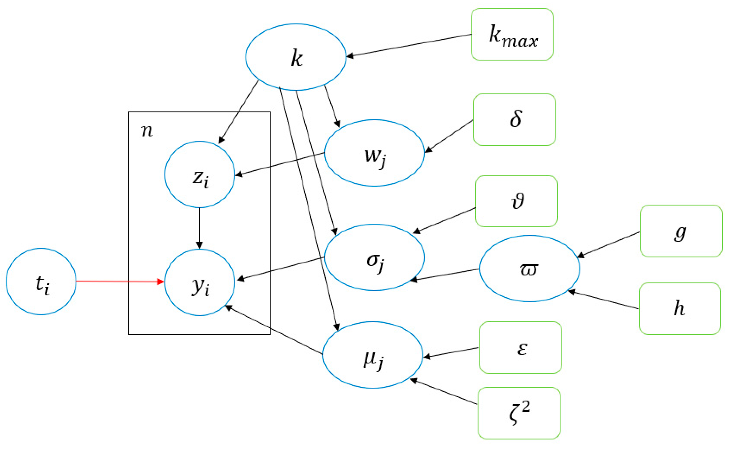
Our hierarchical model can be displayed as a directed acyclic graph (DAG), as shown in Figure 1.

Figure 1. Graphical representation of the Bayesian hierarchical finite EV-I mixture distribution. Nodes in this graph represent random variables, green boxes are fixed hyperparameters, boxes indicate repetition (with the number of repetitions in the upper left), arrows describe conditional dependencies between variables, and the red arrow describes a variable transformation.

4.3. RJMCMC Move Types for EV-I Mixture Distribution

It was mentioned in Section 3.2 that the Algorithm 1, which moves (a), (b), (c), and (d), can be run in parallel. This section will explain in more detail moves (e) and (f), namely split and combine moves, and birth and death moves.

4.3.1. Split and Combine Moves

For move (e), we choose between split or combine, with the probabilities $b_k$ and $d_k=1-b_k$, respectively, depending on $k$. Note that $d_1=0$ and $b_{k_{\max }}=0$, where $k_{\max }$ is the maximum value for $k$; otherwise, we choose $b_k=d_k=0.5$, for $k=1,2,\cdots ,k_{\max }-1$. The combining proposal works as follows: choose two components $j_1$ and $j_2$, where ${\mu }_1<{\mu }_2$ with no other ${\mu }_j\in \left[{\mu }_1,{\mu }_2\right]$. If these components are combined, we reduce $k$ by 1, which forms a new component $j^{\ast }$ containing all the observation previously allocated to $j_1$ and $j_2$, and then creates values for $w_{j^{\ast }}$, ${\mu }_{j^{\ast }}$, and ${\sigma }_{j^{\ast }}$ by preserving the first two moments, as follows:

$$\begin{array}{c}{w}_{j^{\ast }}=w_{j_1}+w_{j_2}\\ w_{j^{\ast }}{\mu }_{j^{\ast }}=w_{j_1}{\mu }_{j_1}+w_{j_2}{\mu }_{j_2}\\ w_{j^{\ast }}\left({\mu }_{j^{\ast }}^2+{\sigma }_{j^{\ast }}\right)=w_{j_1}\left({\mu }_{j_1}^2+{\sigma }_{j_1}\right)+w_{j_2}\left({\mu }_{j_2}^2+{\sigma }_{j_2}\right).\end{array}\}$$

(28)

The splitting proposal works as follows: a random $j^{\ast }$ component is selected then split into two new components, $j_1$ and $j_2$, with the weights and parameters ($w_{j_1}$, ${\mu }_{j_1}$, ${\sigma }_{j_1}$) and ($w_{j_2}$, ${\mu }_{j_2}$, ${\sigma }_{j_2}$), respectively, conforming to Equation (28). Based on this information, we have three degrees of freedom, so we generate three random numbers $u=\left(u_1,u_2,u_3\right)$, where $u_1~\mathrm{Beta}\left(2,2\right)$, $u_2~\mathrm{Beta}\left(2,2\right)$, and $u_3~\mathrm{Beta}\left(1,1\right)$ [16]. Then, split transformations are defined as follows:

$$\begin{array}{c}{w}_{j_1}=w_{j^{\ast }}{u}_1,w_{j_2}=w_{j^{\ast }}\left(1-u_1\right)\\ {\mu }_{j_1}={\mu }_{j^{\ast }}-u_2\sqrt{{\sigma }_{j^{\ast }}}\sqrt{\frac{w_{j_2}}{w_{j_1}}},{\mu }_{j_2}={\mu }_{j^{\ast }}+u_2\sqrt{{\sigma }_{j^{\ast }}}\sqrt{\frac{w_{j_1}}{w_{j_2}}}\\ {\sigma }_{j_1}=u_3\left(1-u_2^2\right){\sigma }_{j^{\ast }}\frac{w_{j^{\ast }}}{w_{j_1}},{\sigma }_{j_2}=\left(1-u_3\right)\left(1-u_2^2\right){\sigma }_{j^{\ast }}\frac{w_{j^{\ast }}}{w_{j_2}}.\end{array}\}$$

(29)

Then, we compute the acceptance probabilities of split and combine moves: $\min \left\{1,A\right\}$ and $\min \left\{1,A^{-1}\right\}$, respectively. According to Equation (9), we obtain $A$ as in Equation (30):

$$\begin{array}{ll}A& =\frac{\mathrm{Pr}\left(z,w,k+1,\theta ,\epsilon ,\zeta ,\vartheta ,\varpi |y\right)d_{k+1}}{\mathrm{Pr}\left(z,w,k,\theta ,\epsilon ,\zeta ,\vartheta ,\varpi |y\right)b_k{p}_{alloc}q\left(u\right)}\left|\frac{\partial {\Delta }^{\ast }}{\partial \left(\Delta ,u\right)}\right|\\ & =\mathrm{likelihood}\mathrm{ratio}\left[\frac{f\left(k+1\right)}{f(k)}\right]\left(k+1\right)\frac{w_{j_1}{}^{\delta +l_1-1}{w}_{j_2}{}^{\delta +l_2-1}}{w_{j^{\ast }}{}^{\delta +l_1+l_2-1}B\left(\delta ,k\delta \right)}\\ & \times {\left(\frac{1}{2\pi {\zeta }^2}\right)}^{\frac{1}{2}}{e}^{-\frac{1}{2{\zeta }^2}\left[{\left({\mu }_{j_1}-\epsilon \right)}^2+{\left({\mu }_{j_2}-\epsilon \right)}^2-{\left({\mu }_{j^{\ast }}-\epsilon \right)}^2\right]}\\ & \times \frac{{\varpi }^{\vartheta }}{\Gamma \left(\vartheta \right)}{\left(\frac{{\sigma }_{j^{\ast }}}{{\sigma }_{j_1}{\sigma }_{j_2}}\right)}^{\vartheta +1}\exp \left(-\varpi \left(\frac{1}{{\sigma }_{j_1}}+\frac{1}{{\sigma }_{j_2}}-\frac{1}{{\sigma }_{j^{\ast }}}\right)\right)\\ & \times \frac{d_{k+1}}{b_k{p}_{alloc}}\frac{1}{g_{2,2}\left(u_1\right)g_{2,2}\left(u_2\right)g_{1,1}\left(u_3\right)}\\ & \times \frac{w_{j^{\ast }}\left|{\mu }_{j_1}-{\mu }_{j_2}\right|{\sigma }_{j_1}{\sigma }_{j_2}}{u_2\left(1-u_2^2\right)u_3\left(1-u_3\right){\sigma }_{j^{\ast }}}\end{array},$$

(30)

where $k$ is the number of components before the split, $l_1$ and $l_2$ are the numbers of observations proposed to be assigned to $j_1$ and $j_2$, $B\left(\cdot ,\cdot \right)$ is the beta function, $p_{alloc}$ is the probability that this particular allocation is made, $g_{p,q}$ is the beta $\left(p,q\right)$ density, the $\left(k+1\right)$-factor in the second line is the ratio $\frac{\left(k+1\right)!}{k!}$ from the order statistics densities for the location-scale parameters $\left(\mu ,\sigma \right)$ [16], and the other terms have been fully explained in Appendix B and Appendix C.

4.3.2. Birth and Death Moves

The following is an explanation of move (f), namely birth and death moves. These moves are simpler than split and combine moves [16]. The first step consists of making a random choice between birth and death, with the same probabilities $b_k$ and $d_k$ as stated above. For birth, the proposed new component has parameters ${\mu }_{j^{\ast }}$ and ${\sigma }_{j^{\ast }}^2$, which are generated from the associated prior distributions shown in Equations (18) and (19), respectively. The weight of the new component $w_{j^{\ast }}$ follows a beta distribution, $w_{j^{\ast }}\sim \mathrm{Beta}\left(1,k\right)$. To remain valid for the constraint ${\displaystyle \sum _{j=1}^k{w}_j+w_{j^{\ast }}=1}$, the previous weights $w_j$ for $j=1,2,\cdots ,k$ must be rescaled by multiplying all by $\left(1-w_{j^{\ast }}\right)$. Therefore, ${\left(1-w_{j^{\ast }}\right)}^k$ is the determinant of Jacobian matrix corresponding to the birth move. For the opposite move, namely the death move, we randomly choose any empty component to remove. This step always considers the constraint that the remaining weights are rescaled to sum 1. The acceptance probabilities of the birth and death moves: $\min \left\{1,A\right\}$ and $\min \left\{1,A^{-1}\right\}$, respectively. According to Equation (9), we obtain $A$ as in Equation (31):

$$A=\frac{\mathrm{Pr}\left(k+1\right)}{\mathrm{Pr}\left(k\right)}\frac{1}{B\left(k\delta ,\delta \right)}{w}_{j^{\ast }}^{\delta -1}{\left(1-w_{j^{\ast }}\right)}^{n+k\delta -k}\left(k+1\right)\frac{d_{k+1}}{b_k\left(k_0+1\right)}\frac{1}{g_{1,k}\left(w_{j^{\ast }}\right)}{\left(1-w_{j^{\ast }}\right)}^k,$$

(31)

where $k_0$ is the number of empty components before birth, and $B\left(\cdot ,\cdot \right)$ is the Beta function.

5. Simulation Study

In this section, we have 16 scenarios, namely Weibull mixture distribution with two components, three components, four components, and five components, each of which is generated with a sample of 125, 250, 500, and 1000 per component. Detailed descriptions of each scenario are given in Table 1, where the “Parameter of EV-I distribution” column is transformed from the “Parameter of Weibull distribution” column.

Table 1. Sixteen scenarios of the Weibull mixture distribution and their transformation into the EV-I mixture distribution.

Scenario	Number of Components	Component	Number of Generated Data	Parameter of Weibull Distribution		Parameter of EV-I Distribution
				$\mathit{\eta }$	$\mathit{\lambda }$	$\mathit{\mu }$	$\mathit{\sigma }$
1	2	1st	125	1	exp(−2)	−2	1
		2nd	125	1/0.5	exp(0)	0	0.5
2	2	1st	250	1	exp(−2)	−2	1
		2nd	250	1/0.5	exp(0)	0	0.5
3	2	1st	500	1	exp(−2)	−2	1
		2nd	500	1/0.5	exp(0)	0	0.5
4	2	1st	1000	1	exp(−2)	−2	1
		2nd	1000	1/0.5	exp(0)	0	0.5
5	3	1st	125	1	exp(−2)	−2	1
		2nd	125	1/0.5	exp(0)	0	0.5
		3rd	125	1/1.5	exp(3)	3	1.5
6	3	1st	250	1	exp(−2)	−2	1
		2nd	250	1/0.5	exp(0)	0	0.5
		3rd	250	1/1.5	exp(3)	3	1.5
7	3	1st	500	1	exp(−2)	−2	1
		2nd	500	1/0.5	exp(0)	0	0.5
		3rd	500	1/1.5	exp(3)	3	1.5
8	3	1st	1000	1	exp(−2)	−2	1
		2nd	1000	1/0.5	exp(0)	0	0.5
		3rd	1000	1/1.5	exp(3)	3	1.5
9	4	1st	125	1	exp(−2)	−2	1
		2nd	125	1/0.5	exp(0)	0	0.5
		3rd	125	1/1.5	exp(3)	3	1.5
		4th	125	1/0.2	exp(5)	5	0.2
10	4	1st	250	1	exp(−2)	−2	1
		2nd	250	1/0.5	exp(0)	0	0.5
		3rd	250	1/1.5	exp(3)	3	1.5
		4th	250	1/0.2	exp(5)	5	0.2
11	4	1st	500	1	exp(−2)	−2	1
		2nd	500	1/0.5	exp(0)	0	0.5
		3rd	500	1/1.5	exp(3)	3	1.5
		4th	500	1/0.2	exp(5)	5	0.2
12	4	1st	1000	1	exp(−2)	−2	1
		2nd	1000	1/0.5	exp(0)	0	0.5
		3rd	1000	1/1.5	exp(3)	3	1.5
		4th	1000	1/0.2	exp(5)	5	0.2
13	5	1st	125	1	exp(−2)	−2	1
		2nd	125	1/0.5	exp(0)	0	0.5
		3rd	125	1/1.5	exp(3)	3	1.5
		4th	125	1/0.2	exp(5)	5	0.2
		5th	125	1	exp(7)	7	1
14	5	1st	250	1	exp(−2)	−2	1
		2nd	250	1/0.5	exp(0)	0	0.5
		3rd	250	1/1.5	exp(3)	3	1.5
		4th	250	1/0.2	exp(5)	5	0.2
		5th	250	1	exp(7)	7	1
15	5	1st	500	1	exp(−2)	−2	1
		2nd	500	1/0.5	exp(0)	0	0.5
		3rd	500	1/1.5	exp(3)	3	1.5
		4th	500	1/0.2	exp(5)	5	0.2
		5th	500	1	exp(7)	7	1
16	5	1st	1000	1	exp(−2)	−2	1
		2nd	1000	1/0.5	exp(0)	0	0.5
		3rd	1000	1/1.5	exp(3)	3	1.5
		4th	1000	1/0.2	exp(5)	5	0.2
		5th	1000	1	exp(7)	7	1

In these scenarios, our specific choices for the hyperparameters were $\zeta =R$, $\vartheta =2$, $g=0.2$, $h=\frac{10}{R^2}$, $\delta =1$, and $k_{\max }=30$, where $R$ and $\epsilon$ are the length and midpoint (median) of the observed data, respectively (see Richardson and Green [16]). Based on the selection of the hyperparameters, we performed an analysis with 200,000 sweeps. With these 200,000 sweeps, we got a value of $k$ as high as 200,000. From this, we took the most frequently occurring (mode) of $k$. Then, we replicated this step 500 times. Thus, we already had one mode $k$ for each replication. Finally, we had 500 $k$ and we calculated them as a percentage. The results of grouping the mixture components can be seen in Table 2, while the parameter estimation results can be seen in Table 3. Based on Table 2, each scenario provides a grouping with an accuracy level of at least 95%; the accuracy level is not 100% only when the sample size is 125 per component. Based on Table 3, it can be seen that the estimated parameters are close to their real parameters for all scenarios. Note: details of the computer and time required for the running simulation study are given in Appendix D.

Table 2. Summary of the results of grouping the EV-I mixture distribution with 200,000 sweeps and replicated 500 times.

Scenario	Number of Components	Sample Size (per Component)	$\mathit{k}=1\left(\mathit{\%}\right)$	$\mathit{k}=2\left(\mathit{\%}\right)$	$\mathit{k}=3\left(\mathit{\%}\right)$	$\mathit{k}=4\left(\mathit{\%}\right)$	$\mathit{k}=5\left(\mathit{\%}\right)$
1	2	125	0	100	0	0	0
2	2	250	0	100	0	0	0
3	2	500	0	100	0	0	0
4	2	1000	0	100	0	0	0
5	3	125	0.8	4.2	95	0	0
6	3	250	0	0	100	0	0
7	3	500	0	0	100	0	0
8	3	1000	0	0	100	0	0
9	4	125	0	0	3.2	96.8	0
10	4	250	0	0	0	100	0
11	4	500	0	0	0	100	0
12	4	1000	0	0	0	100	0
13	5	125	0	0	0	2.4	97.6
14	5	250	0	0	0	0	100
15	5	500	0	0	0	0	100
16	5	1000	0	0	0	0	100

Table 3. Parameter estimation of 16 scenarios, where $\mu$, $\sigma$, and $w$ are the real parameters and $\widehat{\mu }$, $\widehat{\sigma }$, and $\widehat{w}$ are the estimated parameters.

Scenario	Number of Components	Component	Number of Generated Data	Parameter of EV-I Distribution			Estimated Parameter of EV-I Distribution
				$$\mathit{\mu }$$	$$\mathit{\sigma }$$	$$\mathit{w}$$	$$\widehat{\mathit{\mu }}$$	$$\widehat{\mathit{\sigma }}$$	$$\widehat{\mathit{w}}$$
1	2	1st	125	−2	1	0.5	−1.9483	1.019	0.498
		2nd	125	0	0.5	0.5	−0.2771	0.5077	0.502
2	2	1st	250	−2	1	0.5	−2.0034	0.9911	0.4978
		2nd	250	0	0.5	0.5	0.0266	0.4911	0.5022
3	2	1st	500	−2	1	0.5	−2.0009	0.9959	0.5024
		2nd	500	0	0.5	0.5	−0.037	0.4942	0.4976
4	2	1st	1000	−2	1	0.5	−2	1.0023	0.4998
		2nd	1000	0	0.5	0.5	−0.002	0.5082	0.5002
5	3	1st	125	−2	1	0.3333	−1.9736	1.004	0.336
		2nd	125	0	0.5	0.3333	0.005	0.5009	0.328
		3rd	125	3	1.5	0.3333	2.9974	1.4818	0.336
6	3	1st	250	−2	1	0.3333	−1.9734	1.0019	0.3376
		2nd	250	0	0.5	0.3333	0.0179	0.5115	0.3296
		3rd	250	3	1.5	0.3333	3.038	1.5129	0.3328
7	3	1st	500	−2	1	0.3333	−1.9598	0.9935	0.332
		2nd	500	0	0.5	0.3333	−0.0049	0.5162	0.3295
		3rd	500	3	1.5	0.3333	3.021	1.5046	0.3385
8	3	1st	1000	−2	1	0.3333	−2.0062	1	0.3346
		2nd	1000	0	0.5	0.3333	0.0324	0.4943	0.3331
		3rd	1000	3	1.5	0.3333	3.0292	1.5013	0.3323
9	4	1st	125	−2	1	0.25	−1.9909	1.0021	0.2568
		2nd	125	0	0.5	0.25	−0.0563	0.4958	0.2461
		3rd	125	3	1.5	0.25	3.0346	1.497	0.2452
		4th	125	5	0.2	0.25	5.0297	0.205	0.2519
10	4	1st	250	−2	1	0.25	−2.028	0.9977	0.246
		2nd	250	0	0.5	0.25	−0.0213	0.4975	0.2484
		3rd	250	3	1.5	0.25	2.9958	1.496	0.2486
		4th	250	5	0.2	0.25	5.0453	0.2054	0.257
11	4	1st	500	−2	1	0.25	−2.0375	1.0029	0.2499
		2nd	500	0	0.5	0.25	−0.0127	0.4979	0.2489
		3rd	500	3	1.5	0.25	2.987	1.499	0.249
		4th	500	5	0.2	0.25	5.0461	0.2035	0.2522
12	4	1st	1000	−2	1	0.25	−2.023	1.0001	0.2506
		2nd	1000	0	0.5	0.25	0.0266	0.5048	0.2507
		3rd	1000	3	1.5	0.25	2.9932	1.4988	0.2496
		4th	1000	5	0.2	0.25	5.0021	0.1985	0.2491
13	5	1st	125	−2	1	0.2	−1.9904	0.9984	0.1953
		2nd	125	0	0.5	0.2	−0.0613	0.4978	0.1948
		3rd	125	3	1.5	0.2	3.0027	1.4953	0.1909
		4th	125	5	0.2	0.2	5.0289	0.2024	0.1926
		5th	125	7	1	0.2	6.9631	0.9953	0.2264
14	5	1st	250	−2	1	0.2	−2.0178	0.9991	0.1952
		2nd	250	0	0.5	0.2	0.0599	0.498	0.1969
		3rd	250	3	1.5	0.2	3.0547	1.4995	0.2026
		4th	250	5	0.2	0.2	4.9164	0.2005	0.1997
		5th	250	7	1	0.2	6.952	0.9979	0.2056
15	5	1st	500	−2	1	0.2	−2.0065	0.996	0.1992
		2nd	500	0	0.5	0.2	0.0085	0.4998	0.2033
		3rd	500	3	1.5	0.2	3.0289	1.5015	0.1974
		4th	500	5	0.2	0.2	5.0036	0.1965	0.1983
		5th	500	7	1	0.2	7.057	0.9978	0.2018
16	5	1st	1000	−2	1	0.2	−2.0132	1.0048	0.2
		2nd	1000	0	0.5	0.2	−0.0128	0.5025	0.2009
		3rd	1000	3	1.5	0.2	2.9889	1.5011	0.2002
		4th	1000	5	0.2	0.2	4.9884	0.1999	0.2004
		5th	1000	7	1	0.2	7.0045	0.9996	0.1985

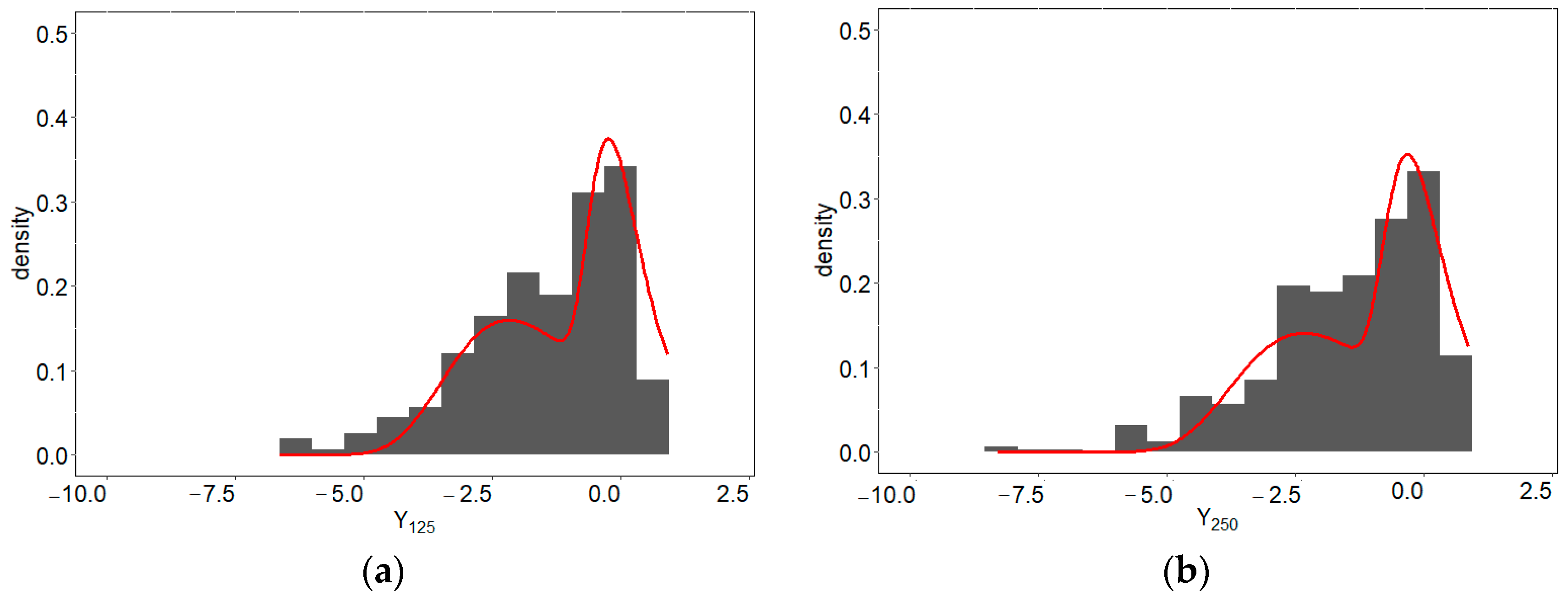
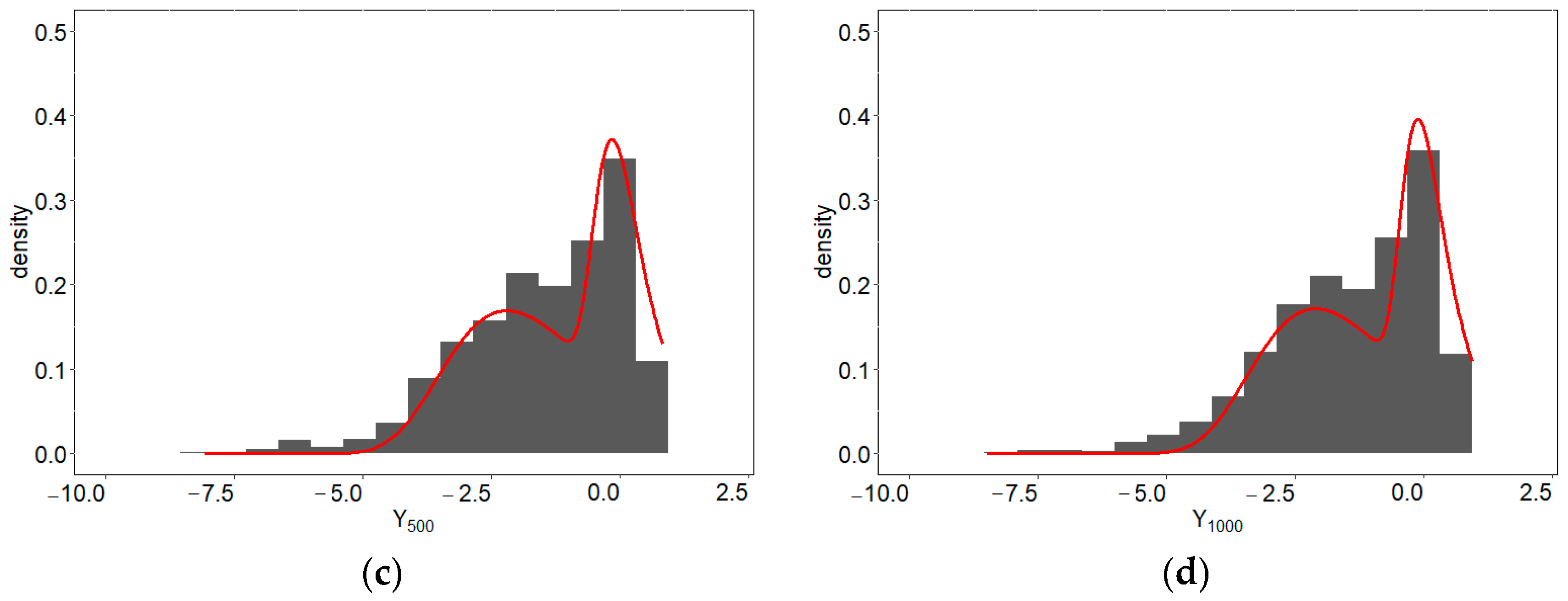
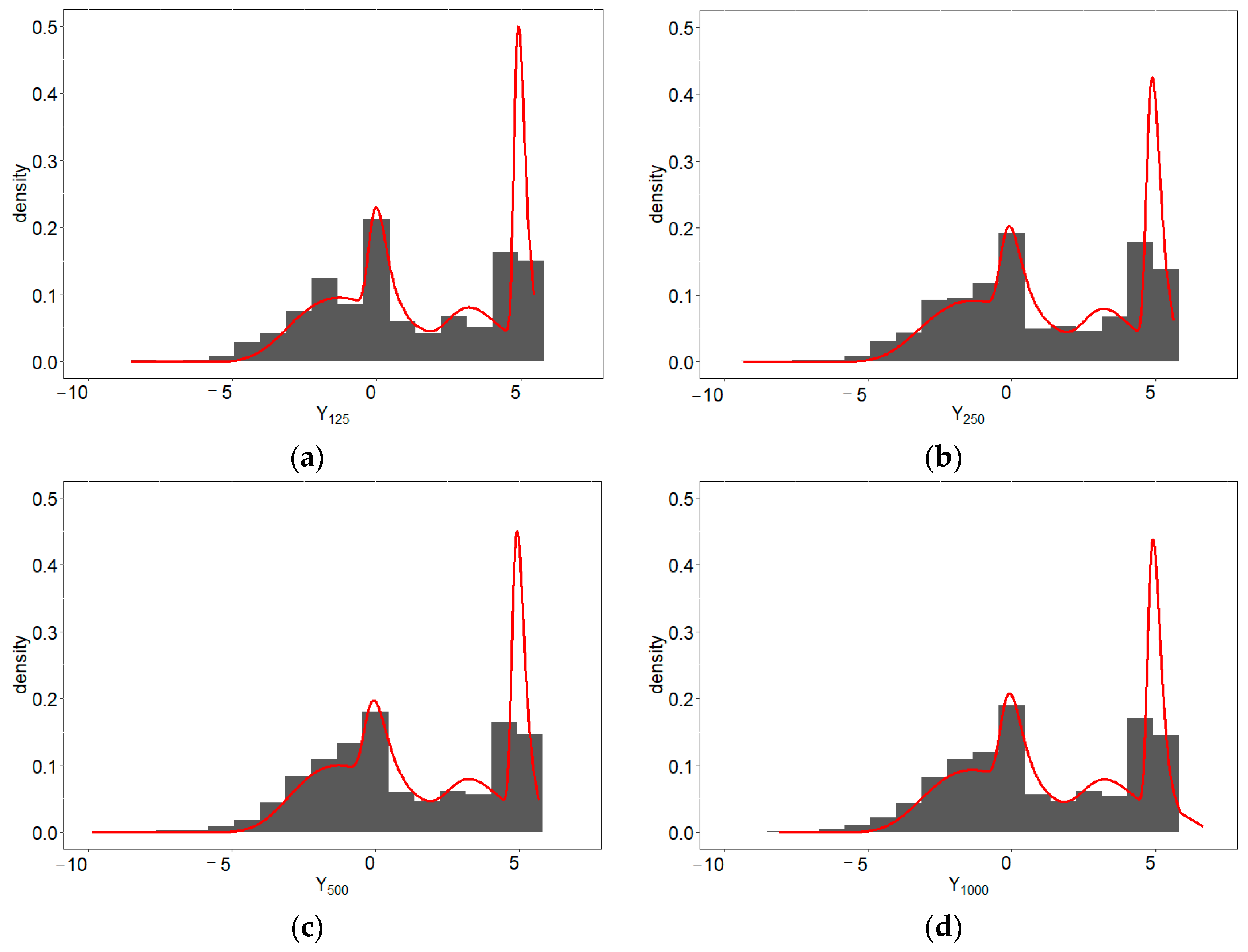
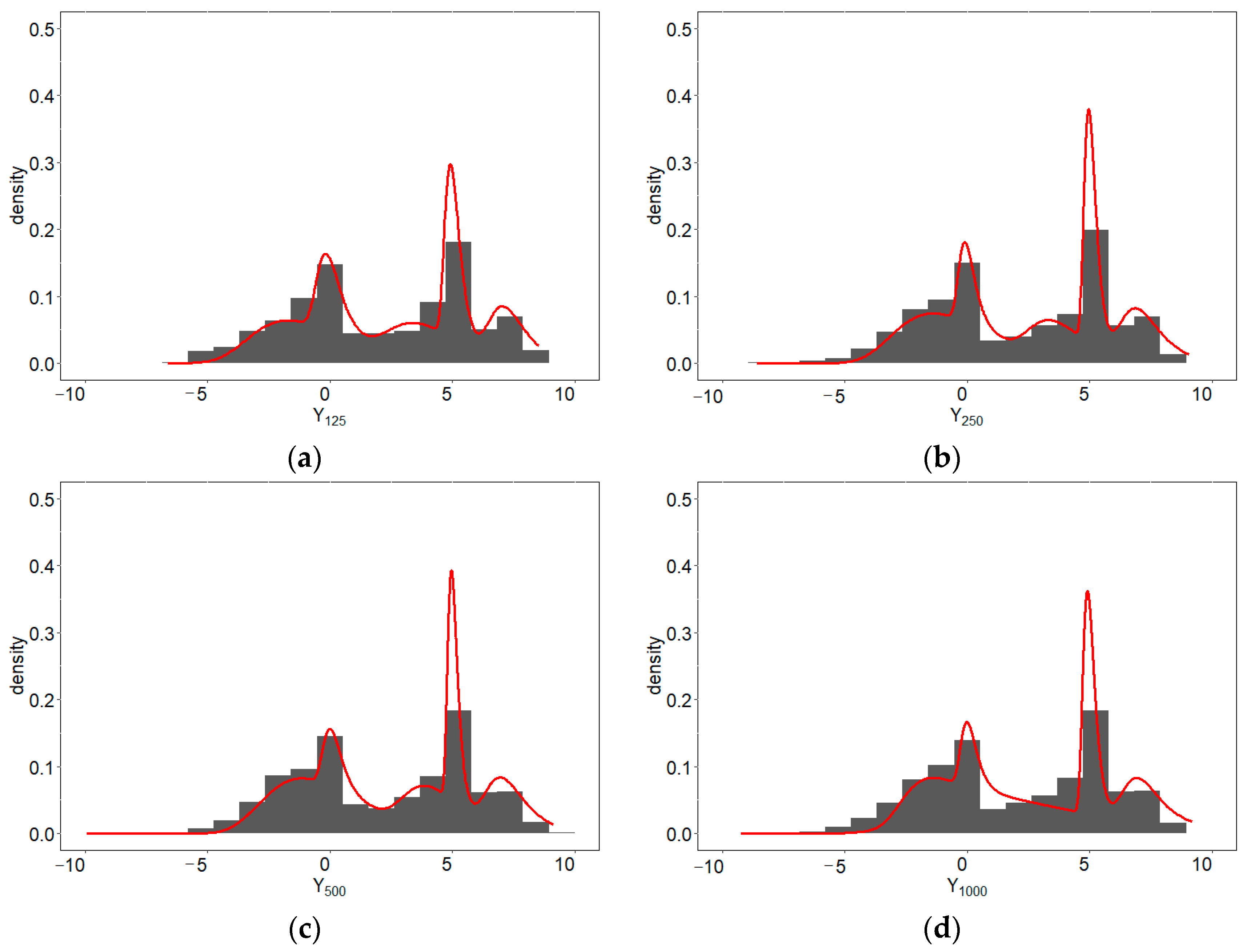
Besides displaying the results of grouping in Table 2 and parameter estimation results in Table 3, we also provide an overview of the histogram and predictive density for each scenario. Histograms and predictive densities for the first to fourth scenarios can be seen in Figure 2a–d, the fifth to eighth scenarios in Figure 3a–d, the ninth to twelfth scenarios in Figure 4a–d, and the thirteenth to sixteenth scenarios in Figure 5a–d.

Figure 2. Histograms and predictive densities for the two-component EV-I mixture distribution with (a) 125, (b) 250, (c) 500, and (d) 1000 samples per component.

Figure 3. Histograms and predictive densities for the three-component EV-I mixture distribution with (a) 125, (b) 250, (c) 500, and (d) 1000 samples per component.

Figure 4. Histograms and predictive densities for the four-component EV-I mixture distribution with (a) 125, (b) 250, (c) 500, and (d) 1000 samples per component.

Figure 5. Histograms and predictive densities for the five-component EV-I mixture distribution with (a) 125, (b) 250, (c) 500, and (d) 1000 samples per component.

6. Misspecification Cases

For the simulation study, we provided 16 scenarios to validate our proposed algorithm. In this section, we provide the opposite—i.e., we intentionally generate data that are not derived from the Weibull distribution and then analyze them using our proposed algorithm. We generate two datasets taken from different distributions. The first dataset is taken from a double-exponential distribution with location and scale parameters of 0 and 1, respectively, and the second dataset is taken from a logistic distribution with location-scale parameters of 2 and 0.4, respectively. Each of these datasets has as many as 1000 data points from the distribution.

We used the EV-I mixture and Gaussian mixture distributions to analyze the data described above. We used the same hyperparameters as in the simulation study section because the double-exponential and logistic distributions both have location and scale parameters. To compare the performance between the EV-I mixture and Gaussian mixture distributions, we used the Kullback–Leibler divergence; a complete explanation and formula for the Kullback–Leibler divergence (KLD) can be found in Van Erven and Harremos [73]. In the simple case, the KLD value of 0 indicates that the true values with fitted densities have identical quantities of information. Thus, the smaller the KLD value, the more identical the true and fitted densities are.

The posterior distribution of $k$ for the misspecification cases data can be seen in Table 4. Based on Table 4, the data that we generate are detected with multimodal data, even though the data we generate are unimodal. Then, in Table 5 can be seen the comparison of KLD for EV-I mixture distribution and Gaussian mixture distribution. Based on Table 5, it can be concluded that the EV-I mixture distribution covers more than the Gaussian mixture distribution for these data.

Table 4. Posterior distribution of $k$ for misspecification cases data based on mixture model using the EV-I distribution.

Distribution of Random Data	$\mathit{n}$	$\mathbf{Pr}\left(\mathit{k}|\mathit{y}\right)$
Double-exponential (0,1)	1000	$\begin{array}{lllll}\mathrm{Pr}\left(1\right)=0& \mathrm{Pr}\left(2\right)=0.2519& \mathrm{Pr}\left(3\right)=0.2631& \mathrm{Pr}\left(4\right)=0.1703& \mathrm{Pr}\left(5\right)=0.1182\\ \mathrm{Pr}\left(6\right)=0.0789& \mathrm{Pr}\left(7\right)=0.0515& {\displaystyle {\sum }_{\ge 8}}\mathrm{Pr}\left(k|y\right)=0.0661& & \end{array}$
Logistic (2,0.4)	1000	$\begin{array}{lllll}\mathrm{Pr}\left(1\right)=0.1492& \mathrm{Pr}\left(2\right)=0.4960& \mathrm{Pr}\left(3\right)=0.2175& \mathrm{Pr}\left(4\right)=0.0843& \mathrm{Pr}\left(5\right)=0.0318\\ \mathrm{Pr}\left(6\right)=0.0122& \mathrm{Pr}\left(7\right)=0.0055& {\displaystyle {\sum }_{\ge 10}}\mathrm{Pr}\left(k|y\right)=0.0035& & \end{array}$

Table 5. Comparison of Kullback–Leibler divergence using EV-I mixture and Gaussian mixture distributions for misspecification cases data.

Distribution of Random Data	Number of Components	Kullback–Leibler
		EV-I Mixture Distribution	Gaussian Mixture Distribution
Double-exponential (0,1)	2	0.0935	0.5311
	3	0.0789	0.5924
	4	0.0902	0.6840
	5	0.0873	0.3892
	6	0.0789	0.2908
	7	0.0677	0.2471
Logistic (2,0.4)	2	0.0629	0.4920
	3	0.0632	0.3288
	4	0.0760	0.2981
	5	0.0754	0.2765
	6	0.0707	0.2587
	7	0.0633	0.2563

7. Application

7.1. Enzyme, Acidity, and Galaxy Datasets

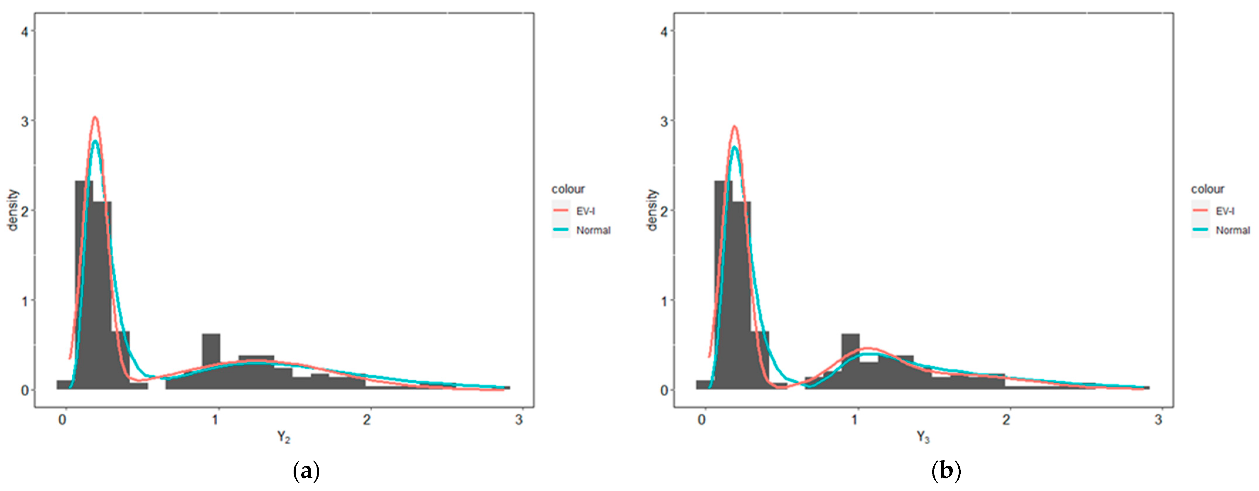
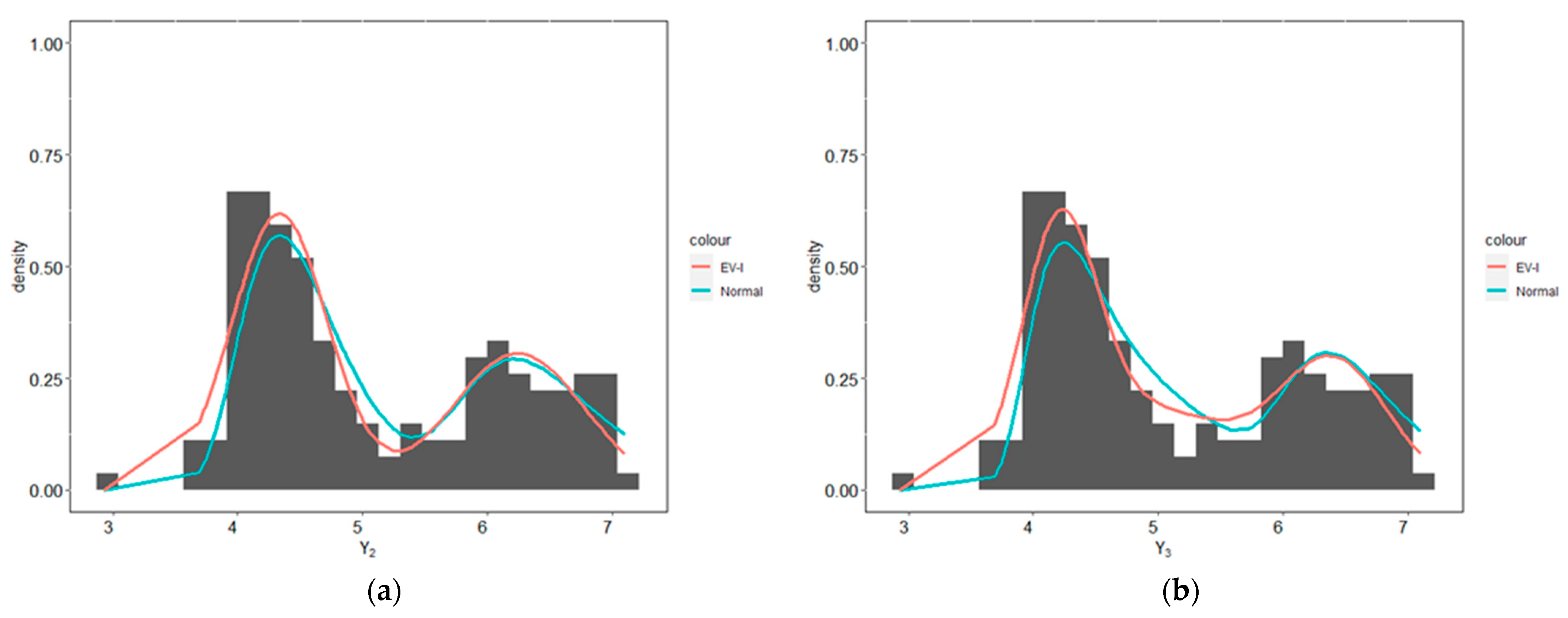
In this section, we analyze enzyme, acidity, and galaxy datasets such as those of Richardson and Green [16] (these three datasets can be obtained from https://people.maths.bris.ac.uk/~mapjg/mixdata, accessed on 22 March 2021). We analyzed the datasets using EV-I mixture distribution with the hyperparameters for enzyme data being $R=2.86$, $\epsilon =1.45$, $\zeta =2.86$, $\vartheta =2$, $g=0.2$, $h=1.22$, $\delta =1$; for acidity data, $R=4.18$, $\epsilon =5.02$, $\zeta =4.18$, $\vartheta =2$, $g=0.2$, $h=0.573$, $\delta =1$; and for galaxy data, $R=25.11$, $\epsilon =21.73$, $\zeta =25.11$, $\vartheta =2$, $g=0.2$, $h=0.016$, $\delta =1$; for these three datasets, we used $k_{\max }=30$. The provisions for selecting these hyperparameters are explained in the Section 5. The posterior distribution of $k$ for all three datasets can be seen in Table 6. Then, we compared the predictive densities of the enzyme, acidity, and galaxy datasets using the EV-I mixture and the Gaussian mixture distributions, which can be seen in Figure 6, Figure 7 and Figure 8. Visually, based on Figure 6, Figure 7 and Figure 8, it can be seen that the EV-I mixture distribution has better coverage than the Gaussian mixture distribution. Then, by using the KLD, it can be seen in Table 7, that the EV-I mixture distribution covers more than the Gaussian mixture distribution.

Table 6. Posterior distribution of $k$ for enzyme, acidity, and galaxy datasets based on mixture model using the EV-I distribution.

Dataset	$\mathit{n}$	$\mathbf{Pr}\left(\mathit{k}|\mathit{y}\right)$
Enzyme	155	$\begin{array}{lllll}\mathrm{Pr}\left(1\right)=0& \mathrm{Pr}\left(2\right)=0.0181& \mathrm{Pr}\left(3\right)=0.2444& \mathrm{Pr}\left(4\right)=0.3232& \mathrm{Pr}\left(5\right)=0.2232\\ \mathrm{Pr}\left(6\right)=0.1135& \mathrm{Pr}\left(7\right)=0.0484& {\displaystyle {\sum }_{\ge 8}\mathrm{Pr}\left(k|y\right)}=0.0292& & \end{array}$
Acidity	245	$\begin{array}{lllll}\mathrm{Pr}\left(1\right)=0& \mathrm{Pr}\left(2\right)=0.0663& \mathrm{Pr}\left(3\right)=0.2470& \mathrm{Pr}\left(4\right)=0.2486& \mathrm{Pr}\left(5\right)=0.1890\\ \mathrm{Pr}\left(6\right)=0.1197& \mathrm{Pr}\left(7\right)=0.0685& {\displaystyle {\sum }_{\ge 8}\mathrm{Pr}\left(k|y\right)}=0.0609& & \end{array}$
Galaxy	82	$\begin{array}{lllll}\mathrm{Pr}\left(1\right)=5\times {10}^{-6}& \mathrm{Pr}\left(2\right)=0.0004& \mathrm{Pr}\left(3\right)=0.0649& \mathrm{Pr}\left(4\right)=0.1410& \mathrm{Pr}\left(5\right)=0.1993\\ \mathrm{Pr}\left(6\right)=0.2095& \mathrm{Pr}\left(7\right)=0.1708& {\displaystyle {\sum }_{\ge 8}\mathrm{Pr}\left(k|y\right)}=0.2141& & \end{array}$

Figure 6. Predictive densities for enzyme data using the EV-I mixture and the Gaussian mixture distributions with (a) two components, (b) three components, (c) four components, (d) five components, (e) six components, and (f) seven components.

Figure 7. Predictive densities for acidity data using the EV-I mixture and the Gaussian mixture distributions with (a) two components, (b) three components, (c) four components, (d) five components, (e) six components, and (f) seven components.

Figure 8. Predictive densities for galaxy data using the EV-I mixture and the Gaussian mixture distributions with (a) two components, (b) three components, (c) four components, (d) five components, (e) six components, and (f) seven components.

Table 7. Comparison of Kullback–Leibler divergence using EV-I mixture and Gaussian mixture distributions for enzyme, acidity, and galaxy datasets.

Dataset	Number of Components	Kullback–Leibler
		EV-I Mixture Distribution	Gaussian Mixture Distribution
Enzyme	2	0.3699	0.7173
	3	0.2670	0.5673
	4	0.6710	0.7992
	5	0.7657	0.9251
	6	2.0578	2.5590
	7	3.4676	3.6022
Acidity	2	0.6508	1.5108
	3	0.5785	1.2076
	4	1.0884	1.4265
	5	1.2894	1.4491
	6	1.2604	1.3877
	7	1.2102	1.3409
Galaxy	2	0.1692	0.2071
	3	0.0880	0.1445
	4	0.0771	0.1542
	5	0.1469	0.1556
	6	0.2005	0.2266
	7	0.2648	0.4460

7.2. Dengue Hemorrhagic Fever (DHF) in Eastern Surabaya, East Java, Indonesia

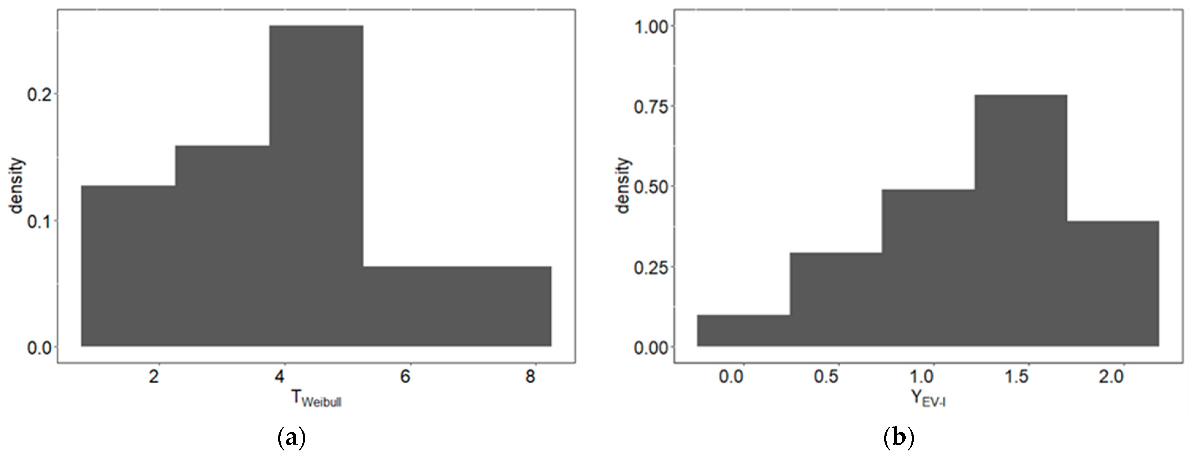
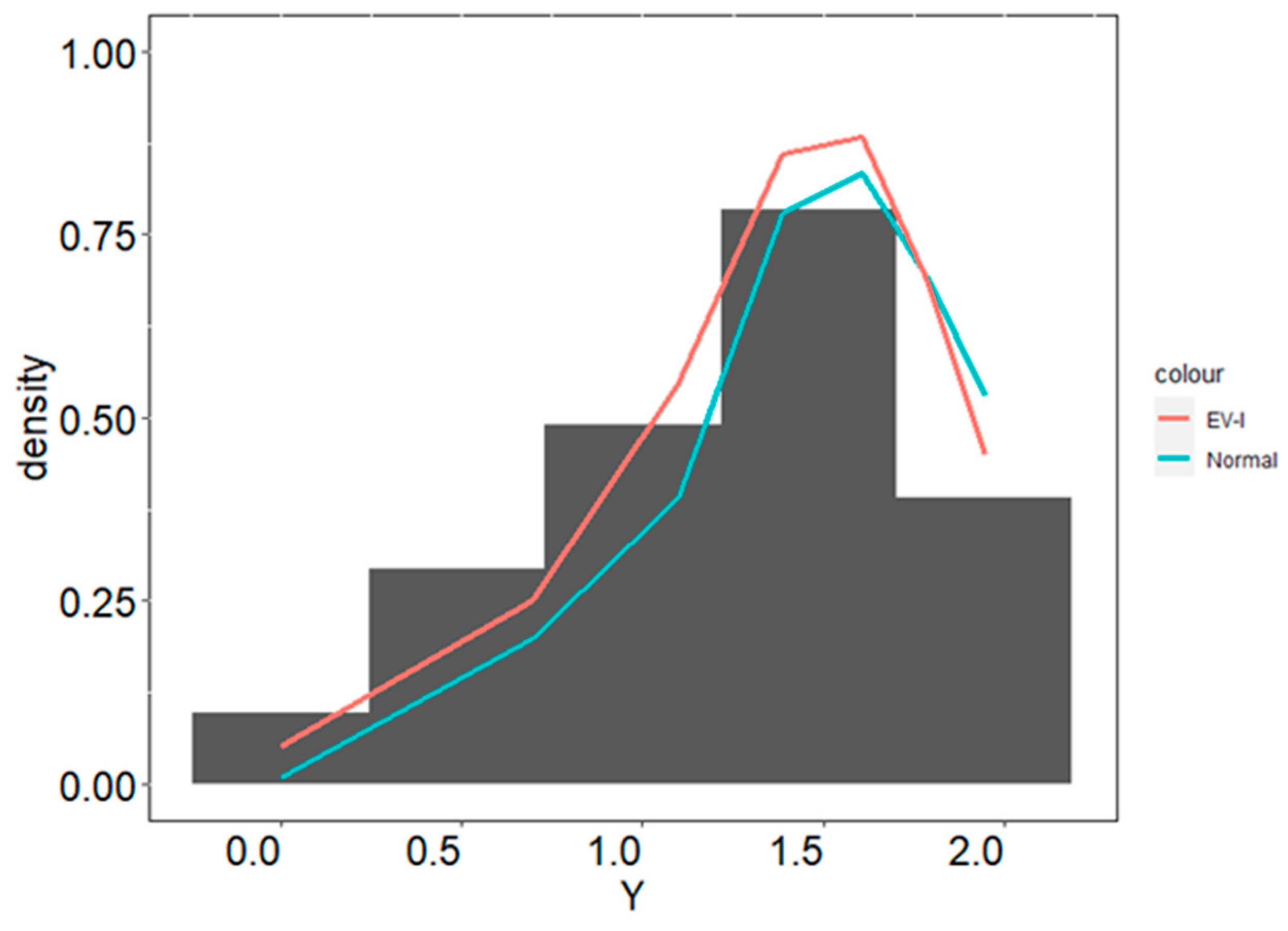
In this section, we apply the EV-I mixture distribution using RJMCMC to a real dataset. These data are the time until patient recovery from dengue hemorrhagic fever (DHF). We obtained the secondary data from medical records from Dr. Soetomo Hospital, Surabaya, East Java, Indonesia. The data concern patients in eastern Surabaya, which consists of seven subdistricts. Our data consist of 21 cases, with each case widespread over each subdistrict. The histogram of the spread of DHF in each subdistrict can be seen in the research conducted by Rantini et al. [36]. It was explained in their study that the data have a Weibull distribution. Whether the data are multimodal or not is unknown. The histogram of our original data is shown in Figure 9a.

Figure 9. Histograms of DHF data in seven subdistricts in eastern Surabaya: (a) original data with Weibull distribution and (b) transformation of the original data into EV-I distribution.

To determine the number of mixture components in our data, we applied the NG-RJMCMC algorithm. Of course, the first step was to transform the original data into a location-scale family, which can be seen in Figure 9b. Then, for our transformed data, we used the hyperparameters $R=1.9459$, $\epsilon =1.3863$, $\zeta =1.9459$, $\vartheta =2$, $g=0.2$, $h=2.6409$, $\delta =1$, and $k_{\max }=30$. Then, we did all six moves type on the data with 200,000 sweeps. The results of the grouping are shown in Table 8. Based on Table 8, the DHF data in eastern Surabaya have a multimodal pattern with the highest probability of having four components.

Table 8. Summary of the results of grouping for DHF data in eastern Surabaya using the EV-I mixture distribution.

$\mathit{n}$

$\mathbf{Pr}\left(\mathit{k}|\mathit{y}\right)$

21

$\begin{array}{lllll}\mathrm{Pr}\left(1\right)=0.0055& \mathrm{Pr}\left(2\right)=0.0095& \mathrm{Pr}\left(3\right)=0.0068& \mathrm{Pr}\left(4\right)=0.3487& \mathrm{Pr}\left(5\right)=0.2778\\ \mathrm{Pr}\left(6\right)=0.1618& \mathrm{Pr}\left(7\right)=0.0845& \mathrm{Pr}\left(8\right)=0.0454& \mathrm{Pr}\left(9\right)=0.0255& {\displaystyle {\sum }_{\ge 10}\mathrm{Pr}\left(k|y\right)}=0.0345\end{array}$

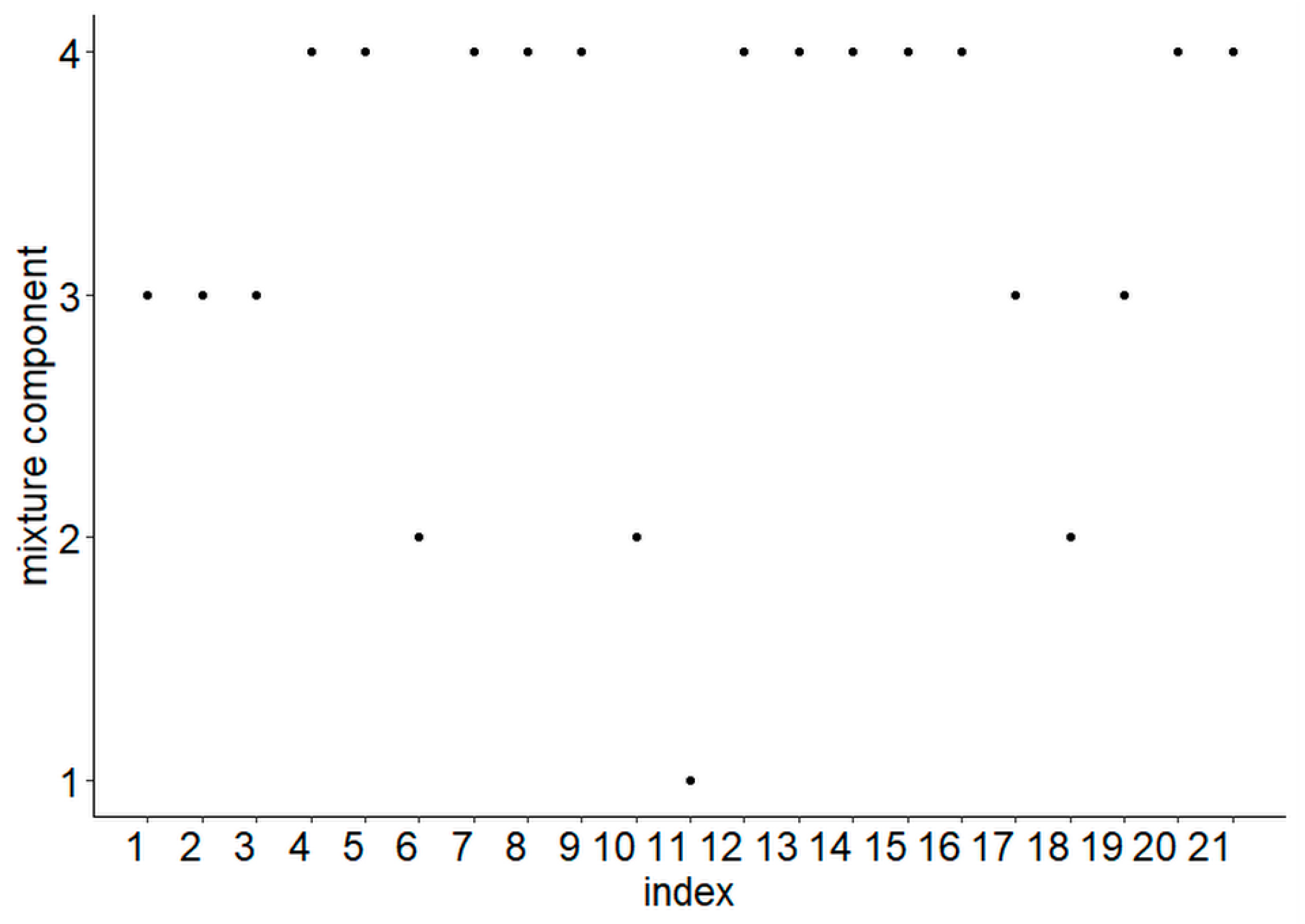
Using the EV-I mixture distribution with four components, the results of the parameter estimation for each component are shown in Table 9. Then, the membership label of each observation in each mixture component is shown in Figure 10. Finally, the analysis was compared using the four-component EV-I mixture distribution and the four-component Gaussian mixture distribution, as shown in Figure 11. According to Table 10 and Figure 11, it can be seen that our data are better covered by using the four-components EV-I mixture distribution.

Table 9. The result of parameter estimation for each component of the EV-I mixture distribution on the DHF data in eastern Surabaya.

Component	$\mathit{w}$	$\mathit{\mu }$	$\mathit{\sigma }$
1st	0.0805	0.0006	0.0053
2nd	0.1614	0.6957	0.0048
3rd	0.2408	1.1022	0.0048
4th	0.5174	1.6265	0.1927

Figure 10. Membership label of each observation on the DHF data in eastern Surabaya using the EV-I mixture distribution with four components.

Figure 11. Comparison of predictive densities for DHF data in eastern Surabaya using the four-component EV-I mixture distribution and the four-component Gaussian mixture distribution.

Table 10. Kullback–Leibler divergence using EV-I mixture and Gaussian mixture distributions for the DHF data in eastern Surabaya.

Number of Components	Kullback–Leibler
	EV-I Mixture Distribution	Gaussian Mixture Distribution
4	0.0711	0.2131

8. Conclusions

We provided an algorithm in the Bayesian mixture analysis. We called it non-Gaussian reversible jump Markov chain Monte Carlo (NG-RJMCMC). Our algorithm is a modification of RJMCMC, where there is a difference in the initial steps, namely changing the original distribution into a location-scale family. This step facilitates the grouping of each observation into the mixture components. Our algorithm allows researchers to easily analyze data that are not from the Gaussian family. In our study, we used Weibull distribution, then transformed it into the EV-I distribution.

To validate our algorithm, we performed 16 scenarios for the EV-I mixture distribution simulation study. The first to fourth scenarios had two components, the fifth to eighth scenarios had three components, the ninth to twelfth scenarios had four components, and the thirteenth to sixteenth scenarios had five components. We generated data in different sizes, ranging from 125 to 1000 samples per mixture component. Next, we analyzed them using a Bayesian analysis with the appropriate prior distributions. We used 200,000 sweeps per scenario and replicated them 500 times. The results of this simulation indicate that each scenario provides a minimum level of accuracy of 95%. Moreover, the estimated parameters come close to the real parameters for all scenarios.

To strengthen the proposed method, we provided misspecification cases. We deliberately generated unimodal data with double-exponential and logistic distributions, then estimated them using the EV-I mixture distribution and Gaussian mixture distribution. The results indicated that the data we generated are multimodally detected. Based on the KLD, the EV-I mixture distribution has better coverage than the Gaussian mixture distribution.

We also implemented our algorithm for real datasets, namely enzyme, acidity, and galaxy datasets. We compared the EV-I mixture distribution with the Gaussian mixture distribution for all three datasets. Based on the KLD, we found that the EV-I mixture distribution has better coverage than the Gaussian mixture distribution. Then, visually, the results also show that the EV-I mixture distribution has better coverage. We also compared the EV-I mixture distribution with the Gaussian mixture distribution for the DHF data in eastern Surabaya. In our previous research, we analyzed the data using the Weibull distribution. We do not know whether the data were identified as multimodal or not. Using our algorithm, we found that the data are multimodal with four components. We also compared the EV-I mixture distribution and the Gaussian mixture distribution. Again, the EV-I mixture distribution indicated better coverage, seen both through the KLD and visually.

References

- Roeder, K. A Graphical Technique for Determining the Number of Components in a Mixture of Normals. J. Am. Stat. Assoc. 1994, 89, 487–495. [Google Scholar] [CrossRef]
- Carreira-Perpinán, M.A.; Williams, C.K.I. On the Number of Modes of a Gaussian Mixture. In Proceedings of the International Conference on Scale-Space Theories in Computer Vision, Isle of Skye, UK, 10–12 June 2003; pp. 625–640. [Google Scholar] [CrossRef]
- Vlassis, N.; Likas, A. A Greedy EM Algorithm for Gaussian Mixture Learning. Neural Process. Lett. 2002, 15, 77–87. [Google Scholar] [CrossRef]
- Jeffries, N.O. A Note on “Testing the Number of Components in a Normal Mixture”. Biometrika 2003, 90, 991–994. [Google Scholar] [CrossRef]
- Lo, Y.; Mendell, N.R.; Rubin, D.B. Testing the Number of Components in a Normal Mixture. Biometrika 2001, 88, 767–778. [Google Scholar] [CrossRef]
- Kasahara, H.; Shimotsu, K. Testing the Number of Components in Normal Mixture Regression Models. J. Am. Stat. Assoc. 2015, 110, 1632–1645. [Google Scholar] [CrossRef]
- McLachlan, G.J. On Bootstrapping the Likelihood Ratio Test Statistic for the Number of Components in a Normal Mixture. J. R. Stat. Soc. Ser. C Appl. Stat. 1987, 36, 318–324. [Google Scholar] [CrossRef]
- Soromenho, G. Comparing Approaches for Testing the Number of Components in a Finite Mixture Model. Comput. Stat. 1994, 9, 65–78. [Google Scholar]
- Bozdogan, H. Choosing the Number of Component Clusters in the Mixture-Model Using a New Informational Complexity Criterion of the Inverse-Fisher Information Matrix. In Information and Classification; Springer: Berlin/Heidelberg, Germany, 1993; pp. 40–54. [Google Scholar] [CrossRef]
- Polymenis, A.; Titterington, D.M. On the Determination of the Number of Components in a Mixture. Stat. Probab. Lett. 1998, 38, 295–298. [Google Scholar] [CrossRef]
- Baudry, J.P.; Raftery, A.E.; Celeux, G.; Lo, K.; Gottardo, R. Combining Mixture Components for Clustering. J. Comput. Graph. Stat. 2010, 19, 332–353. [Google Scholar] [CrossRef]
- Lukočiene, O.; Vermunt, J.K. Determining the Number of Components in Mixture Models for Hierarchical Data. In Studies in Classification, Data Analysis, and Knowledge Organization; Springer: Berlin/Heidelberg, Germany, 2010; pp. 241–249. [Google Scholar] [CrossRef]
- Miller, J.W.; Harrison, M.T. Mixture Models with a Prior on the Number of Components. J. Am. Stat. Assoc. 2018, 113, 340–356. [Google Scholar] [CrossRef] [PubMed]
- Fearnhead, P. Particle Filters for Mixture Models with an Unknown Number of Components. Stat. Comput. 2004, 14, 11–21. [Google Scholar] [CrossRef]
- Mclachlan, G.J.; Rathnayake, S. On the Number of Components in a Gaussian Mixture Model. Wiley Interdiscip. Rev. Data Min. Knowl. Discov. 2014, 4, 341–355. [Google Scholar] [CrossRef]
- Richardson, S.; Green, P.J. On Bayesian Analysis of Mixtures with an Unknown Number of Components. J. R. Stat. Soc. Ser. B Stat. Methodol. 1997, 59, 731–792. [Google Scholar] [CrossRef]
- Astuti, A.B.; Iriawan, N.; Irhamah; Kuswanto, H. Development of Reversible Jump Markov Chain Monte Carlo Algorithm in the Bayesian Mixture Modeling for Microarray Data in Indonesia. In AIP Conference Proceedings; AIP Publishing LLC: Melville, NY, USA, 2017; Volume 1913, p. 20033. [Google Scholar] [CrossRef]
- Liu, R.-Y.; Tao, J.; Shi, N.-Z.; He, X. Bayesian Analysis of the Patterns of Biological Susceptibility via Reversible Jump MCMC Sampling. Comput. Stat. Data Anal. 2011, 55, 1498–1508. [Google Scholar] [CrossRef]
- Bourouis, S.; Al-Osaimi, F.R.; Bouguila, N.; Sallay, H.; Aldosari, F.; Al Mashrgy, M. Bayesian Inference by Reversible Jump MCMC for Clustering Based on Finite Generalized Inverted Dirichlet Mixtures. Soft Comput. 2019, 23, 5799–5813. [Google Scholar] [CrossRef]
- Green, P.J. Reversible Jump Markov Chain Monte Carlo Computation and Bayesian Model Determination. Biometrika 1995, 82, 711–732. [Google Scholar] [CrossRef]
- Sanquer, M.; Chatelain, F.; El-Guedri, M.; Martin, N. A Reversible Jump MCMC Algorithm for Bayesian Curve Fitting by Using Smooth Transition Regression Models. In Proceedings of the 2011 IEEE International Conference on Acoustics, Speech and Signal Processing (ICASSP), Prague, Czech Republic, 22–27 May 2011; pp. 3960–3963. [Google Scholar] [CrossRef]
- Wang, Y.; Zhou, X.; Wang, H.; Li, K.; Yao, L.; Wong, S.T.C. Reversible Jump MCMC Approach for Peak Identification for Stroke SELDI Mass Spectrometry Using Mixture Model. Bioinformatics 2008, 24, i407–i413. [Google Scholar] [CrossRef][Green Version]
- Razul, S.G.; Fitzgerald, W.J.; Andrieu, C. Bayesian Model Selection and Parameter Estimation of Nuclear Emission Spectra Using RJMCMC. Nucl. Instrum. Methods Phys. Res. Sect. A Accel. Spectrometers Detect. Assoc. Equip. 2003, 497, 492–510. [Google Scholar] [CrossRef]
- Karakuş, O.; Kuruoğlu, E.E.; Altınkaya, M.A. Bayesian Volterra System Identification Using Reversible Jump MCMC Algorithm. Signal Process. 2017, 141, 125–136. [Google Scholar] [CrossRef]
- Nasserinejad, K.; van Rosmalen, J.; de Kort, W.; Lesaffre, E. Comparison of Criteria for Choosing the Number of Classes in Bayesian Finite Mixture Models. PLoS ONE 2017, 12, e0168838. [Google Scholar] [CrossRef]
- Zhang, Z.; Chan, K.L.; Wu, Y.; Chen, C. Learning a Multivariate Gaussian Mixture Model with the Reversible Jump MCMC Algorithm. Stat. Comput. 2004, 14, 343–355. [Google Scholar] [CrossRef]
- Kato, Z. Segmentation of Color Images via Reversible Jump MCMC Sampling. Image Vis. Comput. 2008, 26, 361–371. [Google Scholar] [CrossRef]
- Lunn, D.J.; Best, N.; Whittaker, J.C. Generic Reversible Jump MCMC Using Graphical Models. Stat. Comput. 2009, 19, 395. [Google Scholar] [CrossRef]
- Bouguila, N.; Elguebaly, T. A Fully Bayesian Model Based on Reversible Jump MCMC and Finite Beta Mixtures for Clustering. Expert Syst. Appl. 2012, 39, 5946–5959. [Google Scholar] [CrossRef]
- Chen, M.H.; Ibrahim, J.G.; Sinha, D. A New Bayesian Model for Survival Data with a Surviving Fraction. J. Am. Stat. Assoc. 1999, 94, 909–919. [Google Scholar] [CrossRef]
- Banerjee, S.; Carlin, B. Hierarchical Multivariate CAR Models for Spatio-Temporally Correlated Survival Data. Bayesian Stat. 2003, 7, 45–63. [Google Scholar]
- Darmofal, D. Bayesian Spatial Survival Models for Political Event Processes. Am. J. Pol. Sci. 2009, 53, 241–257. [Google Scholar] [CrossRef]
- Motarjem, K.; Mohammadzadeh, M.; Abyar, A. Bayesian Analysis of Spatial Survival Model with Non-Gaussian Random Effect. J. Math. Sci. 2019, 237, 692–701. [Google Scholar] [CrossRef]
- Thamrin, S.A.; McGree, J.M.; Mengersen, K.L. Bayesian Weibull Survival Model for Gene Expression Data. Case Stud. Bayesian Stat. Model. Anal. 2013, 1, 171–185. [Google Scholar] [CrossRef]
- Iriawan, N.; Astutik, S.; Prastyo, D.D. Markov Chain Monte Carlo—Based Approaches for Modeling the Spatial Survival with Conditional Autoregressive (CAR) Frailty. IJCSNS Int. J. Comput. Sci. Netw. Secur. 2010, 10, 211–217. [Google Scholar]
- Rantini, D.; Abdullah, M.N.; Iriawan, N.; Irhamah; Rusli, M. On the Computational Bayesian Survival Spatial Dengue Hemorrhagic Fever (DHF) Modeling with Double-Exponential CAR Frailty. J. Phys. Conf. Ser. 2021, 1722, 012042. [Google Scholar] [CrossRef]
- Rantini, D.; Candrawengi, N.L.P.I.; Iriawan, N.; Irhamah; Rusli, M. On the Computational Bayesian Survival Spatial DHF Modelling with CAR Frailty. In AIP Conference Proceedings; AIP Publishing LLC: Melville, NY, USA, 2021; Volume 2329, p. 60028. [Google Scholar] [CrossRef]
- Villa-Covarrubias, B.; Piña-Monarrez, M.R.; Barraza-Contreras, J.M.; Baro-Tijerina, M. Stress-Based Weibull Method to Select a Ball Bearing and Determine Its Actual Reliability. Appl. Sci. 2020, 10, 8100. [Google Scholar] [CrossRef]
- Zamora-Antuñano, M.A.; Mendoza-Herbert, O.; Culebro-Pérez, M.; Rodríguez-Morales, A.; Rodríguez-Reséndiz, J.; Gonzalez-Duran, J.E.E.; Mendez-Lozano, N.; Gonzalez-Gutierrez, C.A. Reliable Method to Detect Alloy Soldering Fractures under Accelerated Life Test. Appl. Sci. 2019, 9, 3208. [Google Scholar] [CrossRef]
- Tsionas, E.G. Bayesian Analysis of Finite Mixtures of Weibull Distributions. Commun. Stat. Theory Methods 2002, 31, 37–48. [Google Scholar] [CrossRef]
- Marín, J.M.; Rodríguez-Bernal, M.T.; Wiper, M.P. Using Weibull Mixture Distributions to Model Heterogeneous Survival Data. Commun. Stat. Simul. Comput. 2005, 34, 673–684. [Google Scholar] [CrossRef]
- Greenhouse, J.B.; Wolfe, R.A. A Competing Risks Derivation of a Mixture Model for the Analysis of Survival Data. Commun. Stat. Methods 1984, 13, 3133–3154. [Google Scholar] [CrossRef]
- Liao, J.J.Z.; Liu, G.F. A Flexible Parametric Survival Model for Fitting Time to Event Data in Clinical Trials. Pharm. Stat. 2019, 18, 555–567. [Google Scholar] [CrossRef]
- Zhang, Q.; Hua, C.; Xu, G. A Mixture Weibull Proportional Hazard Model for Mechanical System Failure Prediction Utilising Lifetime and Monitoring Data. Mech. Syst. Signal Process 2014, 43, 103–112. [Google Scholar] [CrossRef]
- Elmahdy, E.E. A New Approach for Weibull Modeling for Reliability Life Data Analysis. Appl. Math. Comput. 2015, 250, 708–720. [Google Scholar] [CrossRef]
- Farcomeni, A.; Nardi, A. A Two-Component Weibull Mixture to Model Early and Late Mortality in a Bayesian Framework. Comput. Stat. Data Anal. 2010, 54, 416–428. [Google Scholar] [CrossRef]
- Phillips, N.; Coldman, A.; McBride, M.L. Estimating Cancer Prevalence Using Mixture Models for Cancer Survival. Stat. Med. 2002, 21, 1257–1270. [Google Scholar] [CrossRef]
- Lambert, P.C.; Dickman, P.W.; Weston, C.L.; Thompson, J.R. Estimating the Cure Fraction in Population-based Cancer Studies by Using Finite Mixture Models. J. R. Stat. Soc. Ser. C Appl. Stat. 2010, 59, 35–55. [Google Scholar] [CrossRef]
- Sy, J.P.; Taylor, J.M.G. Estimation in a Cox Proportional Hazards Cure Model. Biometrics 2000, 56, 227–236. [Google Scholar] [CrossRef] [PubMed]
- Franco, M.; Balakrishnan, N.; Kundu, D.; Vivo, J.-M. Generalized Mixtures of Weibull Components. Test 2014, 23, 515–535. [Google Scholar] [CrossRef]
- Bučar, T.; Nagode, M.; Fajdiga, M. Reliability Approximation Using Finite Weibull Mixture Distributions. Reliab. Eng. Syst. Saf. 2004, 84, 241–251. [Google Scholar] [CrossRef]
- Newcombe, P.J.; Raza Ali, H.; Blows, F.M.; Provenzano, E.; Pharoah, P.D.; Caldas, C.; Richardson, S. Weibull Regression with Bayesian Variable Selection to Identify Prognostic Tumour Markers of Breast Cancer Survival. Stat. Methods Med. Res. 2017, 26, 414–436. [Google Scholar] [CrossRef]
- Denis, M.; Molinari, N. Free Knot Splines with RJMCMC in Survival Data Analysis. Commun. Stat. Theory Methods 2010, 39, 2617–2629. [Google Scholar] [CrossRef]
- Mallet, C.; Lafarge, F.; Bretar, F.; Soergel, U.; Heipke, C. Lidar Waveform Modeling Using a Marked Point Process. In Proceedings of the Conference on Image Processing, ICIP, Cairo, Egypt, 7–10 November 2009; pp. 1713–1716. [Google Scholar] [CrossRef]
- Mitra, D.; Balakrishnan, N. Statistical Inference Based on Left Truncated and Interval Censored Data from Log-Location-Scale Family of Distributions. Commun. Stat. Simul. Comput. 2019, 50, 1073–1093. [Google Scholar] [CrossRef]
- Balakrishnan, N.; Ng, H.K.T.; Kannan, N. Goodness-of-Fit Tests Based on Spacings for Progressively Type-II Censored Data from a General Location-Scale Distribution. IEEE Trans. Reliab. 2004, 53, 349–356. [Google Scholar] [CrossRef]
- Castro-Kuriss, C. On a Goodness-of-Fit Test for Censored Data from a Location-Scale Distribution with Applications. Chil. J. Stat. 2011, 2, 115–136. [Google Scholar]
- Bouguila, N.; Elguebaly, T. A Bayesian Approach for Texture Images Classification and Retrieval. In Proceedings of the International Conference on Multimedia Computing and Systems, Ouarzazate, Morocco, 7–9 April 2011; pp. 1–6. [Google Scholar] [CrossRef]
- Naulet, Z.; Barat, É. Some Aspects of Symmetric Gamma Process Mixtures. Bayesian Anal. 2018, 13, 703–720. [Google Scholar] [CrossRef]
- Jo, S.; Roh, T.; Choi, T. Bayesian Spectral Analysis Models for Quantile Regression with Dirichlet Process Mixtures. J. Nonparametr. Stat. 2016, 28, 177–206. [Google Scholar] [CrossRef]
- Kobayashi, G.; Kozumi, H. Bayesian Analysis of Quantile Regression for Censored Dynamic Panel Data. Comput. Stat. 2012, 27, 359–380. [Google Scholar] [CrossRef]
- Gruet, M.A.; Philppe, A.; Robert, C.P. Mcmc Control Spreadsheets for Exponential Mixture Estimation? J. Comput. Graph. Stat. 1999, 8, 298–317. [Google Scholar] [CrossRef]
- Ulrich, W.; Nakadai, R.; Matthews, T.J.; Kubota, Y. The Two-Parameter Weibull Distribution as a Universal Tool to Model the Variation in Species Relative Abundances. Ecol. Complex. 2018, 36, 110–116. [Google Scholar] [CrossRef]
- Scholz, F.W. Inference for the Weibull Distribution: A Tutorial. Quant. Methods Psychol. 2015, 11, 148–173. [Google Scholar] [CrossRef]
- Zhang, J.; Ng, H.K.T.; Balakrishnan, N. Statistical Inference of Component Lifetimes with Location-Scale Distributions from Censored System Failure Data with Known Signature. IEEE Trans. Reliab. 2015, 64, 613–626. [Google Scholar] [CrossRef]
- Park, H.W.; Sohn, H. Parameter Estimation of the Generalized Extreme Value Distribution for Structural Health Monitoring. Probabilistic Eng. Mech. 2006, 21, 366–376. [Google Scholar] [CrossRef]
- Loaiciga, H.A.; Leipnik, R.B. Analysis of Extreme Hydrologic Events with Gumbel Distributions: Marginal and Additive Cases. Stoch. Environ. Res. Risk Assess. 1999, 13, 251–259. [Google Scholar] [CrossRef]
- Banerjee, A.; Kundu, D. Inference Based on Type-II Hybrid Censored Data from a Weibull Distribution. IEEE Trans. Reliab. 2008, 57, 369–378. [Google Scholar] [CrossRef]
- Yoon, S.; Cho, W.; Heo, J.H.; Kim, C.E. A Full Bayesian Approach to Generalized Maximum Likelihood Estimation of Generalized Extreme Value Distribution. Stoch. Environ. Res. Risk Assess. 2010, 24, 761–770. [Google Scholar] [CrossRef]
- Coles, S.G.; Tawn, J.A. A Bayesian Analysis of Extreme Rainfall Data. Appl. Stat. 1996, 45, 463. [Google Scholar] [CrossRef]
- Tancredi, A.; Anderson, C.; O’Hagan, A. Accounting for Threshold Uncertainty in Extreme Value Estimation. Extremes 2006, 9, 87–106. [Google Scholar] [CrossRef]
- Robert, C.P. The Bayesian Choice: From Decision—Theoretic Foundations to Computational Implementation; Springer Science & Business Media: New York, NY, USA, 2007; Volume 91. [Google Scholar]
- Van Erven, T.; Harremos, P. Rényi Divergence and Kullback-Leibler Divergence. IEEE Trans. Inf. Theory 2014, 60, 3797–3820. [Google Scholar] [CrossRef]
Publisher’s Note: MDPI stays neutral with regard to jurisdictional claims in published maps and institutional affiliations. |
© 2021 by the authors. Licensee MDPI, Basel, Switzerland. This article is an open access article distributed under the terms and conditions of the Creative Commons Attribution (CC BY) license (https://creativecommons.org/licenses/by/4.0/).