RCBi-CenterNet: An Absolute Pose Policy for 3D Object Detection in Autonomous Driving

Abstract

3D Object detection is a critical mission of the perception system of a self-driving vehicle. Existing bounding box-based methods are hard to train due to the need to remove duplicated detections in the post-processing stage. In this paper, we propose a center point-based deep neural network (DNN) architecture named RCBi-CenterNet that predicts the absolute pose for each detected object in the 3D world space. RCBi-CenterNet is composed of a recursive composite network with a dual-backbone feature extractor and a bi-directional feature pyramid network (BiFPN) for cross-scale feature fusion. In the detection head, we predict a confidence heatmap that is used to determine the position of detected objects. The other pose information, including depth and orientation, is regressed. We conducted extensive experiments on the Peking University/Baidu-Autonomous Driving dataset, which contains more than 60,000 labeled 3D vehicle instances from 5277 real-world images, and each vehicle object is annotated with the absolute pose described by the six degrees of freedom (6DOF). We validated the design choices of various data augmentation methods and the backbone options. Through an ablation study and an overall comparison with the state-of-the-art (SOTA), namely CenterNet, we showed that the proposed RCBi-CenterNet presents performance gains of 2.16%, 2.76%, and 5.24% in Top 1, Top 3, and Top 10 mean average precision (mAP). The model and the result could serve as a credible benchmark for future research in center point-based object detection.

1. Introduction

Object detection is at the heart of numerous computer vision applications such as face detection [1], video surveillance [2], optical character recognition [3], object counting/tracking [4,5], etc. In autonomous driving [6], the core mission of the perception system of a vehicle computer is to detect nearby objects in real-time and make the optimal driving decisions such as path planning and collision avoidance. Self-driving cars have been in the spotlight and gained explosive development during the past decade [7]. Despite technological advancement, the self-driving system is still far from reliable and trustworthy. Several recent accidents of autonomous vehicles are caused by object misclassification or not being recognized [8]. Therefore, increasing the object detection capability of a self-driving system is one of the highest priorities.

Recent advances in deep learning have elevated the performance of object detection algorithms to a new level [9,10,11,12,13,14]. A wide spectrum of deep learning-based methods has been developed and gained huge success in both academia and industry. However, most prior studies are 2D detection methods that do not provide depth and orientation information, which is required by driving tasks for accurate perception. Figure 1 shows different forms of detection output for a car perception system. A 2D bounding box (Figure 1b) offers limited position information (without depth) and no orientation information. The 3D bounding box in Figure 1c provides more fine-grained pose information. To estimate an accurate 3D mask, Song et al. [15] proposed a keypoint-based approach that learns to convert 2D keypoints (Figure 1d) marked on vehicle objects to corresponding 3D masks (Figure 1e). Regardless of the output format, the absolute 3D pose of a detected object is the most critical datum that should be accurately predicted.

Figure 1. Vehicle object detection: (a) raw image; and (b–e) vehicle objects labeled by 2D, 3D bounding boxes, keypoints, and 3D masks.

A common approach to describe the absolute pose of an object in the world space is the six degrees of freedom (6DOF), which is a six-tuple (yaw, pitch, roll, x, y, z). The first three elements of the 6DOF provide the orientation information and the last three give the position information. A key challenge of using the 6DOF as the prediction target is the lack of annotated datasets for training. 2D images collected by a monocular camera contain rich texture features but lack depth and orientation. 3D cloud points gathered by a Lidar sensor can well represent a 3D scene but lack semantic image features. A camera–Lidar fusion strategy has recently become a popular approach due to its ability to utilize sensory data from both sources, which contain accurate 3D pose data and texture features. The well-known Karlsruhe Institute of Technology and Toyota Technological Institute (KITTI) [16] and its upcoming KITTI 360 [17] datasets are an attempt to offer both 3D and 2D semantics under this integrated setting. Given the limited dataset availability, the Apollocar3d [15] dataset was proposed as an alternative. Vehicle objects in Apollocar3d were annotated with keypoints, which were used to fit the 3D masks. Finally, the resulting 3D masks were used to derive the 3D pose of a vehicle, represented by the 6DOF of the center point of the vehicle. Using this technology, Peking University and Baidu jointly developed the Kaggle Autonomous Driving dataset, which was used in our study.

The current mainstream object detection algorithms predict an object as a bounding box [9,10,11,12]. The learning algorithm can be either one-stage [18] or two-stage [19]. The former works by sliding over an image with pre-arranged bounding boxes, also referred to as anchors, which are directly classified. The latter, on the other hand, extracts image features from each candidate box and then performs classification using those features. Both methods rely on a post-processing operation called non-maxima suppression (NMS), which can effectively eliminate redundant detections but is hard to train and computationally expensive. To address this problem, a new algorithm flavor that focuses on keypoints estimation [13,20] is proposed. A representative approach, CenterNet [20], first predicts the object center point and then regresses other properties such as object size and orientation. Since bounding boxes are not the direct output, NMS is not needed, which speeds up training. CenterNet has been successfully applied to the dataset under investigation and achieved the state-of-the-art (SOTA) performance.

Inspired by the prior efforts, we propose a deep neural network (DNN) architecture for object detection named recursive composite network with a bi-directional feature pyramid. Since the detector part of our model adopts the same idea as CenterNet, we name our model RCBi-CenterNet. The proposed network contains a dual-backbone feature extractor [14] and a bi-directional feature pyramid network (BiFPN) [21] block to extract and fuse cross-scale features. In addition, the model utilizes feedback connections [22] to recursively send output features back to the dual-backbone network to repeat the feature extraction process. This way, an image is looked at and processed twice or more. Due to the inheritance of CenterNet, our model can directly predict the absolute 3D pose of objects without bounding boxes. The contributions of this work are summarized as follows:

• We propose a DNN architecture named RCBi-CenterNet to tackle the object detection problem by predicting the absolute pose of a detected vehicle object in autonomous driving. The model is powered by a recursive composite feature extractor with a BiFPN module to effectively extract, fuse, and represent image features.
• We conducted extensive experiments to justify the design choices of augmentation methods and the optimal backbone. In addition, we evaluated the effect of each integrated module via an ablation study. The overall performance of RCBi-CenterNet outperforms CenterNet by 2.16%, 2.76%, and 5.24% in Top 1, Top 3, and Top 10 mean average precision (mAP), respectively. Our method can serve as a credible benchmark for future research in center point-based objection detection. We open-sourced our code at https://github.com/YixinChen-AI/RCBi_centernet (accessed on 2 June 2020) for public access.

2. Related Work

2.1. Object Detection Based on Candidate Regions

R-CNN (regions with CNN features) [11] has emerged as a groundbreaking method to combine object candidate regions and deep learning in object detection. However, too many candidate regions are produced by only a single image, and every time, after judging the candidate regions, images should be extracted regionally again before being delivered to a deep neural network, making the training slow and hard to optimize. Fast R-CNN [23] is conducted on full images but not by extracting patches of the candidate regions. Generalizable representations of objects can be learned by fast R-CNN when extracting features of the candidate regions on the corresponding deeper feature images. The features obtained by fast R-CNN can be utilized for subsequent recognition and object bounding box regression. R-CNN and fast R-CNN are two algorithms based on the raw images realized by common algorithms in image processing, which is time-consuming. To speed up training, region proposal network (RPN) is adopted to generate object candidate regions in faster R-CNN [24]. The whole object detection and recognition process are contained inside the deep learning network. A sequence-to-sequence model is employed in faster R-CNN to accelerate training. In MR-CNN, s-CNN, and the Loc model [25], detection accuracy is improved in object candidate regions and deep features. Object candidate regions are segmented in different regions, and MR-CNN is conducted to extract the features in these regions to represent the regions together. Deep utilization to candidate regions is employed, and semantic segmentation CNN (s-CNN) is proposed to extract the high-level features from the object feature maps.

2.2. Object Detection Based on Keypoints

To improve the accuracy and speed of network training models in object detection, CenterNet [13] adopts keypoints instead of bounding boxes for object detection. Mobile CenterNet is proposed to be deployed on embedded devices in real industrial application scenarios [26]. HRNet is utilized as a powerful backbone in Mobile CenterNet to decrease the calculation cost and shorten the algorithm’s implementation time. Keypoint triplets are proposed to perceive the internal semantic information of the bounding box. In the backbone CenterNet, prediction boxes are generated by corner keypoint triplets, and scale-aware central regions are employed to define the sizes of the center region. In combination with information extracted from center points, bounding boxes can be detected, while the sizes of the center region are not refined enough [13]. A simpler and more effective center point-based approach is proposed in [20], which utilizes the keypoints to estimate the object center points. Relevant properties are regressed, such as size, 3D location, orientation, and poses.

2.3. Object Detection in Autonomous Driving

The mainstream 3D object detection techniques in autonomous driving can be divided into three categories [27]: monocular detection [28,29,30], Lidar-based detection [31,32], and camera–Lidar fusion [33,34,35,36]. Each line of work has its pros and cons. Monocular detection works by detecting 2D objects in RGB images that help reason in the 3D space to estimate depth and orientation. However, the lack of explicit 3D information from the input limits the localization accuracy. On the other hand, Lidar-based detection aims to detect 3D objects directly from the point cloud sampled from the real world; however, due to the lack of semantic texture information, DNNs cannot learn rich and meaningful features. Camera–Lidar fusion is a hybrid strategy that combines front view images and point cloud to generate interactive and semantic-rich features to train an end-to-end 3D object detector. The majority of detectors developed under the three categories adopt an anchor-based method to predict bounding boxes, and another line of work utilizes a point-based method [20,37] to first predict the center point of an object and then regress other pose information. The point-based detector showed superior performance in both AP and inference time on the COCO dataset [20], compared to the anchor-based methods. This study offers a custom point-based solution of object detection in the autonomous driving domain, which falls into the monocular detection category. The same type of work does not exist in the literature. Our work has the potential to be extended to work in a camera–Lidar fusion setting, where the 3D point coordinates can be obtained directly from the point cloud and projected to the 2D image to serve as an accurate position; in addition, a DNN model can extract rich semantic features the RGB images to boost the detection accuracy.

2.4. 3D Object Datasets

In the previous 3D object datasets [38,39,40,41,42,43], there are several drawbacks such as limited objects in scale, only partial 3D properties, and few objects per image. In the EPFL cars, 20 cars are contained under different viewpoints, while they are captured in a controllable turntable which is quite different from real-time traffic conditions [42]. Non-controllable and more realistic scenes are required in real object detection for autonomous driving cars, and datasets containing natural images [44] collected from Flickr [45] or indoor scenes [46] with Kinect are added in 3D objects [47]. A few hundred indoor images are labeled in the IKEA datasets [44] with 3D furniture models. Twelve rigid categories in PASCAL VOC 2012 images [48] are labeled in PASCAL3D+ [49], and a larger 3D object dataset is proposed by ObjectNet3D [50] with images from ImageNet [51] with 100 categories. These datasets are useful but still cannot meet the real traffic driving scenarios in autonomous driving. Although the KITTI dataset seems to be matched with our requirement, cars in the KITTI dataset [16] are only labeled by a rectangular bounding box, and a lack of fine-grained semantic keypoint is discovered.

3. The Dataset and Learning Task

3.1. Dataset

The dataset used in our study is derived from the ApolloSpace dataset [15] created by the Baidu Robotics and Autonomous Driving Lab (RAL) and Peking University. The dataset consists of more than 60,000 labeled 3D car instances from 5277 real-world images based on industry-grade CAD car models. All images are with high resolution and collected in real traffic environments with diverse driving conditions in four cities of China. Compared to KITTI, the ApolloSpace dataset contains more movable objects (11.7 vs. 4.1 average cars per image). There are some challenging environments in the dataset; for example, two extreme lighting conditions (e.g., dark and bright) appearing in the same image could be caused by the shadow of an overpass [52].

The training data consist of 4262 images, and each comes with a line describing the 3D pose information of all vehicles annotated in the image. The pose information is given as a string with the following format: model type, yaw, pitch, roll, x, y, z, where (yaw, pitch, roll) gives the orientation/rotation information and (x, y, z) provides the position/translation information. The model type indicates the car model that comes with a 3D model, which can help determine the vehicle size and orientation but is not required as a part of the prediction result. Note that some vehicles are not of interest because they are too far/small and are therefore removed from consideration for the task. In addition, the camera intrinsic parameters are provided to facilitate the coordinate conversion between the 3D world space and the 2D image space, as shown in Figure 2.

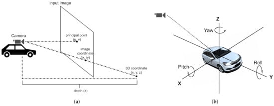
Figure 2. (a) The camera perspective from the top of the autonomous vehicle. All images in the dataset are taken by this camera. The principal point (u, v), at the center of an image, is the point on the image plane onto which the perspective center is projected. With a given camera intrinsic matrix, we can obtain a conversion between a point’s 3D coordinate (x, y, z) in the world space and its 2D coordinate, denoted as (ix, iy), in the image space. (b) Six degrees of freedom (6DOF) can be used to determine the absolute pose of a vehicle in the world space. Rotation around the side-to-side (X) axis is called pitch; rotation around the front-to-back (Y) axis is called roll; and rotation around the vertical (Z) axis is called yaw.

Given the transformed 2D position and orientation data, along with provided car models, the ground truth vehicle annotations can be visualized with a center point and the bottom rectangle of a 3D bounding box, as shown in Figure 3. Note that the bounding boxes are estimated and are only for visualization purposes. We can also plot a distribution of vehicle objects across the dataset, as shown in Figure 4.

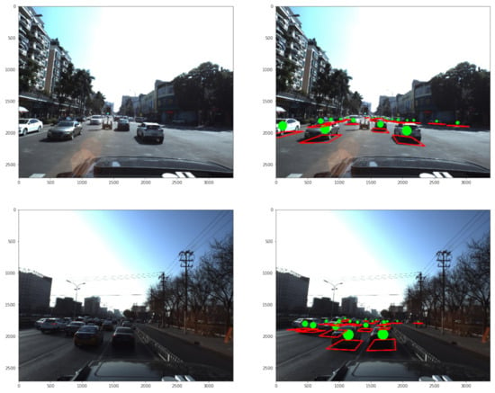
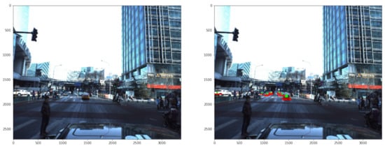
Figure 3. The original sample images (left) and the ones with ground truth labels (right).

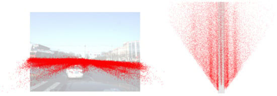
Figure 4. Vehicle object distribution in the dataset from the camera’s view (left) and viewed from the sky (right).

3.2. Learning Task

The task of this challenge is to develop an algorithm to predict the absolute pose of vehicles (6DOF) in an input image collected from a real-world traffic environment. 6DOF is widely used in manufacturing for building a precision positioning system [53], which is also highly desired in autonomous driving. In this dataset, vehicle objects do not present large movement in pitch and roll since the vehicles are on a flat road and roughly at the same level as the camera.

In addition, a confidence score between 0 and 1 should be provided to indicate the chance of a detected vehicle being a real one. In summary, a seven-tuple entry (yaw, pitch, roll, x, y, z, confidence) is used to describe the prediction of a vehicle object.

3.3. Evaluation Metric

Unlike traditional bounding box-based object detection tasks, which use the Intersection over Union (IoU) thresholds to determine true/false positives, this task utilizes the mean average precision (mAP) between the predicted and ground truth pose information as the evaluation metric. To calculate the mAP, we need to obtain the translation distance and the rotation distance between the predicted objects and the solution objects. Let P and $P^{\prime }$ denote the ground truth and predicted center point of an object, respectively. The translation distance between P and $P^{\prime }$ is the Euclidean distance given by $d_{trans}(P,P^{\prime })=\sqrt{{(P_x-P_x^{\prime })}^2+{(P_y-P_y^{\prime })}^2+{(P_z-P_z^{\prime })}^2}$, and the rotation distance $d_{rot}(P,P^{\prime })$ is calculated using the Euclidean distance between the Euler angles. The set of equations are omitted here due to the space limit. Readers with interests can refer to Section 3.2 of [54] for a detailed calculation process.

The resulting distances between all pairs of objects are taken to find out the closest predicted objects to the solution objects. Ten levels of thresholds are then applied to determine a true/false positive. Specifically, given a threshold level that includes a translation and a rotation threshold, if the calculated translation and rotation distances are less than the corresponding translation and rotation thresholds, then the predicted object is said to be a true positive for that threshold level. Otherwise, it is counted as a false positive. Lastly, we can calculate an mAP across all predictions in all of the images for each threshold level and use Top i to represent the mAP for the threshold level i. Note that the higher is a threshold level, the higher are the threshold values and the less accurate is the prediction. For this dataset, the ten rotation threshold levels are 5–50 with a step size 5, and the ten translation threshold levels are 0.01–0.1 with a step size 0.01.

4. RCBi-CenterNet

This section covers the technical details of the proposed RCBi-CenterNet architecture.

4.1. Data Augmentation

To further increase the diversity of the input images and the model’s robustness, we apply the following image processing algorithms to augment the original dataset.

• Contrast limited adaptive histogram equalization (CLAHE) aims at enhancing image contrast effectively by alternating the illumination of the image adaptively, and the presentability of the images can be improved, which is essential for an effective CNN feature extraction process. In this study, we adopted three different magnitudes of contrast enhancement to verify how contrast enhancement can affect the performance of the RCBi-CenterNet. The clip limits are utilized to present the variations, which are 0.005 (low enhancement), 0.01 (moderate enhancement), and 0.02 (high enhancement) [55].
• Random brightness contrast (RBC) is adopted by random factors sampled from a uniform distribution of [0:7; 1:3], generating changes in color.
• Horizontal flip (HFlip) simply mirrors an image in the horizontal direction.
• HFlip+CLAHE means the dataset is firstly augmented by HFlip and CLAHE individually, and then augmented by HFlip and CLAHE combined. The augmented dataset is four times the original one.
• HFlip+RBC means the dataset is firstly augmented by HFlip and RBC individually, and then augmented by HFlip and RBC combined.

4.2. Overall RCBi-CenterNet Architecture

Figure 5 describes the overall architecture of the proposed RCBi-CenterNet, which consists of the following modules:

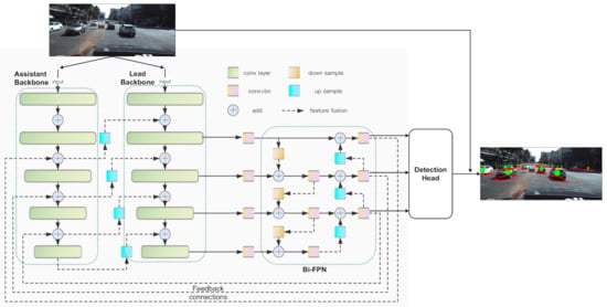
Figure 5. RCBi-CenterNet architecture.

• A feature extractor combines two adjacent networks, including an assistant backbone and a lead backbone that jointly output multi-scale features, which are passed to the subsequent modules.
• A BiFPN is used to fuse multi-scale features in bi-directional pathways to generate more representative features.
• The output of BiFPN is sent back to the assistant backbone via the feedback connections and the previous two modules are repeated to look at the image twice or more, which could enhance the feature representation.

4.3. Dual-Backbone Network

The first module is a dual-backbone network, which is composed of two adjacent backbones with an identical structure. Compared to a single backbone network, using two or more side-by-side backbones has the potential to extract richer semantic features [14] from the images.

The network sends an input image through both backbones, which are assembled through composition connections between the assistant and lead backbones, as shown in Figure 5. Let $B_a$ and $B_l$ denote the assistant and lead backbone, respectively. Let K denote the number of stages for each backbone. The input of the kth stage of $B_l$ is the fusion of $B_l$’s output at stage $k-1$ and $B_a$’s output at stage k, denoted by ${\mathbf{F}}_{k-1}^l$ and ${\mathbf{F}}_k^a$, respectively. Formally, to obtain the output feature map of kth stage of $B_l$, namely ${\mathbf{F}}_k^l$, we have

$${\mathbf{F}}_k^l=C_k^l\left({\mathbf{F}}_{k-1}^l+h\left({\mathbf{F}}_k^a\right)\right)$$

(1)

where $C_k^l$ refers to the convolutional layer at stage k in $B_l$ and function $h(·)$ refers to a composition link that transforms ${\mathbf{F}}_k^a$ by reducing its channels via a $1\times 1$ convolutional operation ($1\times 1$ conv), followed by a batch normalization (BN) layer and an upsample operation to ensure that the resulting tensor $h\left({\mathbf{F}}_k^a\right)$ has the same dimension as ${\mathbf{F}}_{k-1}^l$. This way, the output feature maps of $B_a$ are fused into the input features of each stage of $B_l$ iteratively. Finally, the collection of feature maps $\left\{{\mathbf{F}}_k^l\right|k=1,...,K\}$, generated by $B_l$ and transformed via a $1\times 1$ conv + BN block for dimension shrink, and the resulting outputs, denoted by $\left\{{\mathbf{F}}_k^{\prime }\right|k=1,...,K\}$, are fed into the subsequent module.

4.4. BiFPN-Based Cross-Scale Feature Fusion

The second module is a BiFPN for efficient multi-scale feature fusion. Taking the list of output features from the module one, a BiFPN block employs top-down and bottom-up pathways to aggregate features with different resolutions. Formally, we have

$$\begin{array}{c}\hfill \begin{array}{cc}\hfill & {\mathbf{F}}_k^{\downarrow }=C_{3\times 3}\left({\mathbf{F}}_k^{\prime }+g_{\downarrow }\left({\mathbf{F}}_{k-1}^{\prime }\right)\right)\hfill \\ \hfill & {\mathbf{F}}_k^{\uparrow }=C_{3\times 3}\left({\mathbf{F}}_k^{\downarrow }+g_{\uparrow }\left({\mathbf{F}}_{k-1}^{\downarrow }\right)\right)\hfill \end{array}\end{array}$$

(2)

where $g_{\uparrow }$ and $g_{\downarrow }$ denote the upsample and downsample functions and $C_{3\times 3}$ refers to a $C_{3\times 3}$ conv + BN block. The list of feature maps $\left\{{\mathbf{F}}_k^{\uparrow }\right|k=1,...,K\}$ represents the output feature set of the BiFPN module.

4.5. Recursive Feature Extraction

The dual-backbone network and the BiFPN module represent a base structure for feature extraction in our model, which is adequate for large- and medium-sized objects. To enhance the model’s ability to detect small objects, we adopt the RFP strategy that utilizes feedback connections (marked in Figure 5), which allow a model to look at the input image twice or more. Specifically, the output features of BiFPN are sent back to the dual-backbone network through the feedback connections and fused with the stage outputs of the assistant backbone. This way, the previous two modules are repeated with the knowledge, i.e., features, learned from the first look. The recursive process can be unrolled to an T-step sequential network, where T is the number of repetitions. Figure 6 shows an unrolled two-step sequential network. Our model adopts $T=2$, since an input image is looked at a total of four times due to the joint effect of a dual-backbone network and the RFP. Let the list of feature maps $\left\{{\mathbf{F}}_{k,t}^{\uparrow }\right|k=1,...,K;t=1,...,T\}$ represent the output feature set of the BiFPN module after the tth repetition of the unrolled sequential network. The feature set $\left\{{\mathbf{F}}_{k,T}^{\uparrow }\right\}$ is fed into the detection head for the final prediction.

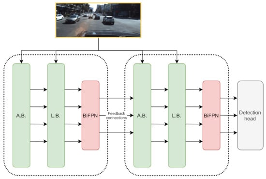
Figure 6. RPF unrolled to a two-step sequential network; A.B. and L.B. refer to assistant backbone and lead backbone, respectively.

4.6. Detection Head

As discussed in Section 3.2, our prediction target is a seven tuple (yaw, pitch, roll, x, y, z, confidence), in which the first six variables describe an absolute pose of a detected vehicle and the last one is a confidence score. The detection head consists of two branches. The first branch predicts a center point heatmap that gives the confidence scores at each location, and the second branch predicts a tensor that regresses the orientation (yaw, pitch, and roll) and the depth (z).

The idea to produce the confidence scores is from Zhou et al. [20]. Let $I\in {\mathbb{R}}^{W\times H\times 3}$ be a $W\times H$ image and let $\mathbf{H}$ be the ground truth center point heatmap $\mathbf{H}\in {[0,1]}^{\frac{W}{R}\times \frac{H}{R}}$, where R is the output stride to scale down the image by a factor of R. For each ground truth center point $p(x,y,z)$ in the 3D world space, we convert it to a 2D point $p^{\prime }(x^{\prime },y^{\prime })$ in the image, and then scale it down to obtain the corresponding location $\overline{p}(\overline{x},\overline{y})$ in the low-resolution heatmap. Let ${\mathbf{H}}_{{\overline{x}}_{+}{\overline{y}}_{+}}$ denote a ground true center point located at $\left({\overline{x}}_{+}{\overline{y}}_{+}\right)$ of the heatmap. We then apply a Gaussian kernel [20]${\mathbf{H}}_{\overline{x}\overline{y}}=exp\left(-\frac{{(\overline{x}-{\overline{x}}_{+})}^2+{(\overline{y}-{\overline{y}}_{+})}^2}{2{\sigma }^2}\right)$, where $\sigma$ denotes the vehicle size-adaptive standard deviation. The Gaussian kernel helps transform each ground truth center point to a circular area in $\mathbf{H}$ so that the near pixels of the center point can also receive a positive score, depending on their closeness to the circle center. This transformation effectively creates more pixels with positive labels and facilitates model training [20]. Part of the learning goal is to generate a center point heatmap ${\mathbf{H}}^{\prime }\in {[0,1]}^{\frac{W}{R}\times \frac{H}{R}}$ to approximate $\mathbf{H}$ and minimize the prediction error. For both $\mathbf{H}$ and ${\mathbf{H}}^{\prime }$, if there is an overlap between two Gaussians, the element-wise maximum is taken. Lastly, given that the positive samples, namely pixels with a value greater than 0.5, are far less than the negative samples, there exists an imbalanced sample distribution. In other words, the majority of an input image is background. Therefore, we adopt focal loss to handle this imbalanced distribution. The loss function is given as follows:

$$L_{\mathbf{H}}=-\frac{1}{S_{\mathbf{H}}}\sum _{\overline{x}\overline{y}}\left({\mathbf{H}}_{\overline{x}\overline{y}}\alpha {(1-{\widehat{\mathbf{H}}}_{\overline{x}\overline{y}})}^{\gamma }log\left({\widehat{\mathbf{H}}}_{\overline{x}\overline{y}}\right)+(1-{\mathbf{H}}_{\overline{x}\overline{y}})(1-\alpha ){\widehat{\mathbf{H}}}_{\overline{x}\overline{y}}^{\gamma }log(1-{\widehat{\mathbf{H}}}_{\overline{x}\overline{y}})\right)$$

(3)

where $\alpha$ and $\gamma$ are hyper-parameters of the focal loss and $S_{\mathbf{H}}$ is the size of the heatmap, which is $\frac{W}{R}\times \frac{H}{R}$.

The other branch of the detection head is to predict the pose information, which is done by regression. Instead of predicting a 3D coordinate $(x,y,z)$ directly, we choose to predict $(\overline{x},\overline{y},z)$, and then convert $\overline{x}$ and $\overline{y}$ into the corresponding 3D coordinates. The output of this branch is a tensor $\widehat{\mathbf{P}}\in {\mathbb{R}}^{\frac{W}{R}\times \frac{H}{R}\times 4}$. We can then define ${\widehat{\mathbf{P}}}_{\overline{x}\overline{y}}=(yaw,pitch,roll,z)$, a four-element tuple, as the orientation and the depth of the vehicle object detected at $(\overline{x},\overline{y})$ in the heatmap. We employ the L1 loss to regress the pose information as follows:

$$L_{\mathbf{P}}=\frac{1}{S_{\mathbf{H}}}\sum _{\overline{x}\overline{y}}\left(∥{\mathbf{P}}_{\overline{x}\overline{y}}-{\widehat{\mathbf{P}}}_{\overline{x}\overline{y}}∥{\mathbf{H}}_{\overline{x}\overline{y}}\right)$$

(4)

Note that both $L_{\mathbf{H}}$ and $L_{\mathbf{P}}$ calculate the loss for a single image. By combining losses (3) and (4), we obtain the overall loss function across the entire training set:

$$L=\sum _{i=1}^m\left(L_{\mathbf{H}}+L_{\mathbf{P}}\right)$$

(5)

where m is the number of images in the training set.

5. Experiments and Result Analysis

The proposed model was evaluated through a series of experiments to validate the effects of different model settings. Specifically, we examined the impact of data augmentation methods and different backbones used in the dual-backbone network of our model. We also compared the performance between our model and the SOTA, namely CenterNet.

Instead of using all ten mAPs, the performance results are reported as Top 1, Top 3, and Top 10 mAPs, which are sufficient to represent a model’s overall performance at various precision levels. Top 1 and Top 10 reflect the performance under the most and least strict threshold settings, while Top 3 was chosen over Top 5 because we intend to emphasize that the model comparison is made more strictly.

5.1. Training Setting

Since the test set of the competition is not provided, we divided the original training set, with 4262 images, into new training and validation sets in the ratio of 4:1. All images in the dataset have the same resolution of 3384 × 2710 pixels and were resized to 576 × 320 pixels. The whole training took 60 epochs. The initial learning rate was set to 3 × 10${}^{-4}$ and was divided by ten at Epochs 45 and 55 to stabilize training. The hyperparameters used by CenterNet [20] were also used in our training: the output stride R was set to 4, while $\alpha$ and $\gamma$ in Equation (3) were set to 2 and 4, respectively. The model and training algorithms were implemented using Pytorch 1.7. All experiments were conducted on a rig with 4xGTX 1080Ti GPUs. It took approximately 11 min per epoch when training the model with the best backbone network Se_ResNet101, adding up to 11 h to finish a total of 60 epochs.

5.2. Comparison of Different Data Augmentation Methods

We adopted CLAHE, RBC, horizon flip (HFlip), HFlip + CLAHE, and HFlip + RBC for data augmentation and compared their effects on the proposed RCBi-CenterNet model. The results are reported in Figure 7. Observations and findings are listed as follows.

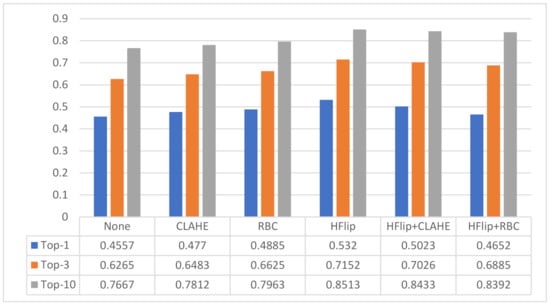
Figure 7. Effects of data augmentation methods.

• All evaluated augmentation methods showed performance improvements to varying degrees, compared to “None”, meaning that data augmentation serves an effective strategy to increase the dataset diversity and allows a model to learn richer features.
• HFlip showed the best result, with 7.43%, 8.87%, and 8.47% improvement for Top 1, Top 3, and Top 10, respectively, compared to the model without augmentation. HFlip is more effective than CLAHE and RBC, potentially due to the fact that HFlip is the only method that changes both the position and orientation of the vehicle objects by mirroring an image in the horizontal direction, creating more objects with different pose information for the model to learn.
• CLAHE and RBC, although not as good as HFlip, presented marginal performance boosts. Neither CLAHE nor RBC creates new pose information, but they do add new color features, which showed a limited but still positive impact.
• Combining with CLAHE and RBC, the hybrid methods HFlip + CLAHE and HFlip + RBC did not show remarkable improvement. HFlip + CLAHE outperformed CLAHE but was worse than HFlip, and HFlip + RBC under-performed compared to both HFlip and RBC applied individually. This result is somehow counter-intuitive since HFlip and the other two focus on different aspects to augment the image features and should work better than each method applied individually.

5.3. Comparison of Different Backbones

We conducted experiments aiming to find an optimal backbone among a list of backbone candidates, including ResNet18, ResNet50, ResNet101, and Se_ResNet101, Se_ResNet101_32 × 4 d. The results are exhibited in Figure 8. Observations and findings are as follows.

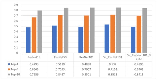
Figure 8. Effects of different backbones used in the dual-backbone feature extractor.

• Among the tested backbones, Se_ResNet101 showed the best mAP in all three indicators. Compared to ResNet101, the addition of a squeeze-and-excitation (SE) block allowed the model to learn channel-wise attentions, leading to significant performance boost.
• By increasing the ResNet depth from 18 to 50, a 4–5% improvement could be achieved in all three indicators. However, further increasing the depth from 50 to 101 showed no obvious improvement, meaning that, as the network depth reaches a certain degree, its impact on model performance is limited. As the number of network layers deepened and the parameters increased, the fitting ability of the neural network became stronger, which meant that the function expressed by it became more complicated and overfitting could occur, leading to a performance drop on the test set.
• With a $32\times 2$ d template, Se_ResNet101_32 × 4 d did not offer positive effect on the performance, compared to Se_ResNet101, thus an increment on convolutional kernels was not helpful.

5.4. Comparison of Different Feature Fusion Methods

To validate the effect of feature fusion strategies, we compared five models, namely CentrNet, CBNet-CentrNet, BiFPN-CentrNet, RFP-CentrNet, and RCBi-CenterNet, in which CBNet-CentrNet employs the dual-backbone feature extractor, BiFPN-CentrNet adds a BiFPN block into CenterNet, and RFP-CenterNet adds feedback connections to CenterNet and enables a two-step sequential network. All five models were evaluated on the same dataset and used the same backbone. Note that CenterNet is regarded as the SOTA as it was one of the models that won the Gold medal of the competition (https://www.kaggle.com/diegojohnson/centernet-objects-as-points, accessed on 20 May 2021). The results are shown in Figure 9. We provide our observations and insights as follows.

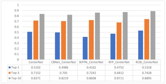
Figure 9. Performance comparison.

• Adding a composite dual-backbone network to CenterNet alone was not effective, reducing the mAP by 1–2%. However, we kept the dual-backbone component because once we removed a backbone from RCBi-CenterNet, a performance drop of 2–4% in all three metrics was observed, meaning that the dual-backbone design worked better with BiFPN and the feedback connections integrated into the same system.
• The addition of BiFPN boosted Top 3 and Top 10 by 0.9% and 2.37%, respectively, and decreasesd Top 1 by 9.4%, meaning that the BiFPN module could help classify more objects with a looser threshold, but its performance in Top 1 was greatly reduced compared to CenterNet.
• The implementation of a recursive network brought down both Top 1 and Top 3 by 3–4%, but boosted Top 10 by 3.4%, presenting a similar effect with BiFPN.
• Combining the dual-backbone and BiFPN modules in a recursive fashion, the resulting RCBi-CenterNet model showed superior performance over CenterNet, with 2.16%, 2.76%, and 5.24% performance gains in Top 1, Top 3, and Top 10, respectively. This result demonstrates that the proposed network architecture can effectively extract, fuse, and represent distinguishable features for object detection in the domain of autonomous driving.

In addition, we provide the inference speed for the five evaluated models in Figure 10. As expected, the inference speed dropped from 23.8 frames per second (FPS) to 13.2 FPS, as we added more feature fusion strategies to the base CenterNet model. Despite the speed degradation, our RCBi_CenterNet can still meet the requirement of real-time inference for practical use. In [56], the authors presented a YOLO-based real-time object detector that runs 13 FPS on the Microsoft HoloLens. Cheng et al. proposed a CenterNet-based model with weighted feature fusion and attention mechanism [57] for object detection and had a speed of 13.5 FPS on four NVIDIA TITAN Xp GPUs. In [58], a mobile CenterNet was developed and achieved a speed of 7 FPS on an NVIDIA TX2. These studies show that the speed of 13.2 FPS for our model is practical. Meanwhile, we realize that there is always a trade-off between accuracy and speed, where speed can be improved with better hardware, but accuracy can only be improved with better architecture design.

Figure 10. Inference speed.

6. Discussion

Building a robust, accurate, and efficient 3D object detector is a critical mission to realize an intelligent perception system of an autonomous vehicle. The mainstream efforts utilize anchor-based methods to predict bounding boxes, which involve inefficient post-processing work, namely NMS, to enumerate a list of candidate object locations and classify each. To address this challenge, recent studies explore a point-based detector that uses key points to estimate the center point of an object and then regress other object properties. A representative work, CenterNet [20], has demonstrated superior performance in both detection accuracy and speed on the COCO dataset, compared to other anchor-based methods. The novelty and efficiency of CenterNet drive us to explore its application in autonomous driving.

In this paper, we develop a center point-based DNN named RCBi-CenterNet for object detection in autonomous driving. The proposed RCBi-CenterNet predicts the center points using a heatmap of confidence scores and selects the peak values to represent detected objects. In addition, our method regresses the object depth and orientation, which describe the absolute pose of an object, along with the position information given by the heatmap. RCBi-CenterNet is powered by a recursive composite network that consists of a dual-backbone module and a BiFPN module for cross-scale feature fusion. We conducted a series of experiments to validate the design choices of various data augmentation methods and backbones and selected HFlip and Se_ResNet101 as the best options for model integration. Finally, an overall comparison between RCBi-CenterNet and the SOTA, CenterNet, is reported. The results show the superiority of RCBi-CenterNet, with 2.16%, 2.76%, and 5.24% performance gains in Top 1, Top 3, and Top 10, respectively, demonstrating the efficacy of the proposed method.

The pitch and roll degrees in the dataset do not carry valuable information since vehicle objects are captured on a flat road and are at the same horizontal level as the camera sensor. This is commonly seen in the current self-driving scenario. However, it should be noted that the usage of 6DOF as a prediction target can be extended to the object detection task in more autonomous driving scenarios, such as unmanned aerial drones (UAV), underwater drones, or even in the outer space, where the absolute 3D position of detected objects, with more meaningful data in all six degrees, can be provided.

This work has the following limitations, which also point out our future directions. First, the performance boost brought by RCBi-CenterNet comes with a cost, i.e., a drop of the detection speed; although the resulting speed, 13.2 FPS, can meet the real-time requirement, it can be further improved. The root cause of the performance drop is the added complexity of the feature extractor, which requires image features to go through multiple layers horizontally, vertically, and recursively. Thus, one direction is to simplify the DNN architecture, keeping the model slim and fast. Second, there are other feature extraction techniques to be tested in our system, such as CNN attention modules [59] and feature interaction [60]. Third, a generative data augmentation method can further enrich the vehicle samples in the original dataset. However, a challenge would be to automatically generate training samples with the 3D position annotations compatible with the existing system. Fourth, it would be interesting to explore the effect of other kernels than the Gaussian kernel. The kernel is a crucial design choice because it decides how the pixels close to the center point are marked as positive in the ground truth heatmap, which determines the sample distribution and directly impacts detection accuracy. Lastly, we plan to investigate a point-based camera–Lidar fusion model, which could offer a promising perspective to complement the current research efforts.

References

- Sun, X.; Wu, P.; Hoi, S.C. Face detection using deep learning: An improved faster RCNN approach. Neurocomputing 2018, 299, 42–50. [Google Scholar] [CrossRef]
- Pérez-Hernández, F.; Tabik, S.; Lamas, A.; Olmos, R.; Fujita, H.; Herrera, F. Object detection binary classifiers methodology based on deep learning to identify small objects handled similarly: Application in video surveillance. Knowl.-Based Syst. 2020, 194, 105590. [Google Scholar] [CrossRef]
- Chaudhuri, A.; Mandaviya, K.; Badelia, P.; Ghosh, S.K. Optical character recognition systems. In Optical Character Recognition Systems for Different Languages with Soft Computing; Springer: Berlin/Heidelberg, Germany, 2017; pp. 9–41. [Google Scholar]
- Onoro-Rubio, D.; López-Sastre, R.J. Towards perspective-free object counting with deep learning. In European Conference on Computer Vision; Springer: Berlin/Heidelberg, Germany, 2016; pp. 615–629. [Google Scholar]
- Du, D.; Qi, Y.; Yu, H.; Yang, Y.; Duan, K.; Li, G.; Zhang, W.; Huang, Q.; Tian, Q. The unmanned aerial vehicle benchmark: Object detection and tracking. In Proceedings of the European Conference on Computer Vision (ECCV), Munich, Germany, 8–14 September 2018; pp. 370–386. [Google Scholar]
- Wang, D.; Devin, C.; Cai, Q.Z.; Yu, F.; Darrell, T. Deep object-centric policies for autonomous driving. In Proceedings of the 2019 International Conference on Robotics and Automation (ICRA), Montreal, QC, Canada, 20–24 May 2019; pp. 8853–8859. [Google Scholar]
- Badue, C.; Guidolini, R.; Carneiro, R.V.; Azevedo, P.; Cardoso, V.B.; Forechi, A.; Jesus, L.; Berriel, R.; Paixao, T.M.; Mutz, F.; et al. Self-driving cars: A survey. Expert Syst. Appl. 2020, 165, 113816. [Google Scholar] [CrossRef]
- Hong, J. Why is artificial intelligence blamed more? Analysis of faulting artificial intelligence for self-driving car accidents in experimental settings. Int. J. Hum.-Comput. Interact. 2020, 36, 1768–1774. [Google Scholar] [CrossRef]
- Krizhevsky, A.; Sutskever, I.; Hinton, G.E. Imagenet classification with deep convolutional neural networks. Adv. Neural Inf. Process. Syst. 2012, 25, 1097–1105. [Google Scholar] [CrossRef]
- Fang, H.S.; Xie, S.; Tai, Y.W.; Lu, C. Rmpe: Regional multi-person pose estimation. In Proceedings of the IEEE International Conference on Computer Vision, Venice, Italy, 22–29 October 2017; pp. 2334–2343. [Google Scholar]
- Girshick, R.; Donahue, J.; Darrell, T.; Malik, J. Rich feature hierarchies for accurate object detection and semantic segmentation. In Proceedings of the IEEE Conference on Computer Vision and Pattern Recognition, Columbus, OH, USA, 24–27 June 2014; pp. 580–587. [Google Scholar]
- Dai, J.; Li, Y.; He, K.; Sun, J. R-fcn: Object detection via region-based fully convolutional networks. arXiv 2016, arXiv:1605.06409. [Google Scholar]
- Duan, K.; Bai, S.; Xie, L.; Qi, H.; Huang, Q.; Tian, Q. Centernet: Keypoint triplets for object detection. In Proceedings of the IEEE/CVF International Conference on Computer Vision, Seoul, Korea, 27 October–2 November 2019; pp. 6569–6578. [Google Scholar]
- Liu, Y.; Wang, Y.; Wang, S.; Liang, T.; Zhao, Q.; Tang, Z.; Ling, H. Cbnet: A novel composite backbone network architecture for object detection. In Proceedings of the AAAI Conference on Artificial Intelligence, New York, NY, USA, 7–12 February 2020; Volume 34, pp. 11653–11660. [Google Scholar]
- Song, X.; Wang, P.; Zhou, D.; Zhu, R.; Guan, C.; Dai, Y.; Su, H.; Li, H.; Yang, R. Apollocar3d: A large 3d car instance understanding benchmark for autonomous driving. In Proceedings of the IEEE/CVF Conference on Computer Vision and Pattern Recognition, Long Beach, CA, USA, 16–20 June 2019; pp. 5452–5462. [Google Scholar]
- Geiger, A.; Lenz, P.; Urtasun, R. Are we ready for autonomous driving? the kitti vision benchmark suite. In Proceedings of the 2012 IEEE Conference on Computer Vision and Pattern Recognition, Providence, RI, USA, 16–21 June 2012; pp. 3354–3361. [Google Scholar]
- Xie, J.; Kiefel, M.; Sun, M.T.; Geiger, A. Semantic instance annotation of street scenes by 3d to 2d label transfer. In Proceedings of the IEEE Conference on Computer Vision and Pattern Recognition, Las Vegas, NV, USA, 26 June–1 July 2016; pp. 3688–3697. [Google Scholar]
- Liu, W.; Anguelov, D.; Erhan, D.; Szegedy, C.; Reed, S.; Fu, C.Y.; Berg, A.C. Ssd: Single shot multibox detector. In European Conference on Computer Vision; Springer: Berlin/Heidelberg, Germany, 2016; pp. 21–37. [Google Scholar]
- Ciresan, D.; Giusti, A.; Gambardella, L.; Schmidhuber, J. Deep neural networks segment neuronal membranes in electron microscopy images. Adv. Neural Inf. Process. Syst. 2012, 25, 2843–2851. [Google Scholar]
- Zhou, X.; Wang, D.; Krähenbühl, P. Objects as points. arXiv 2019, arXiv:1904.07850. [Google Scholar]
- Tan, M.; Pang, R.; Le, Q.V. Efficientdet: Scalable and efficient object detection. In Proceedings of the IEEE/CVF Conference on Computer Vision and Pattern Recognition, Venice, Italy, 14–19 June 2020; pp. 10781–10790. [Google Scholar]
- Qiao, S.; Chen, L.C.; Yuille, A. Detectors: Detecting objects with recursive feature pyramid and switchable atrous convolution. arXiv 2020, arXiv:2006.02334. [Google Scholar]
- Redmon, J.; Divvala, S.; Girshick, R.; Farhadi, A. You only look once: Unified, real-time object detection. In Proceedings of the IEEE Conference on Computer Vision and Pattern Recognition, Las Vegas, NV, USA, 26 June–1 July 2016; pp. 779–788. [Google Scholar]
- Ren, S.; He, K.; Girshick, R.; Sun, J. Faster r-cnn: Towards real-time object detection with region proposal networks. arXiv 2015, arXiv:1506.01497. [Google Scholar] [CrossRef] [PubMed]
- Gidaris, S.; Komodakis, N. Object detection via a multi-region and semantic segmentation-aware cnn model. In Proceedings of the IEEE International Conference on Computer Vision, Santiago, Chile, 11–18 December 2015; pp. 1134–1142. [Google Scholar]
- Yu, J.; Xie, H.; Li, M.; Xie, G.; Yu, Y.; Chen, C.W. Mobile Centernet for Embedded Deep Learning Object Detection. In Proceedings of the 2020 IEEE International Conference on Multimedia & Expo Workshops, (ICMEW), London, UK, 6–10 July 2020; pp. 1–6. [Google Scholar]
- Arnold, E.; Al-Jarrah, O.Y.; Dianati, M.; Fallah, S.; Oxtoby, D.; Mouzakitis, A. A survey on 3d object detection methods for autonomous driving applications. IEEE Trans. Intell. Transp. Syst. 2019, 20, 3782–3795. [Google Scholar] [CrossRef]
- Chen, X.; Kundu, K.; Zhang, Z.; Ma, H.; Fidler, S.; Urtasun, R. Monocular 3d object detection for autonomous driving. In Proceedings of the IEEE Conference on Computer Vision and Pattern Recognition, Las Vegas, NV, USA, 26 June–1 July 2016; pp. 2147–2156. [Google Scholar]
- Simonelli, A.; Bulo, S.R.; Porzi, L.; López-Antequera, M.; Kontschieder, P. Disentangling monocular 3d object detection. In Proceedings of the IEEE/CVF International Conference on Computer Vision, Seoul, Korea, 27 October–2 November 2019; pp. 1991–1999. [Google Scholar]
- Nobis, F.; Brunhuber, F.; Janssen, S.; Betz, J.; Lienkamp, M. Exploring the Capabilities and Limits of 3D Monocular Object Detection-A Study on Simulation and Real World Data. In Proceedings of the 2020 IEEE 23rd International Conference on Intelligent Transportation Systems (ITSC), Rhodes, Greece, 20–23 September 2020; pp. 1–8. [Google Scholar]
- Börcs, A.; Nagy, B.; Benedek, C. Instant object detection in lidar point clouds. IEEE Geosci. Remote Sens. Lett. 2017, 14, 992–996. [Google Scholar] [CrossRef]
- Zhou, Y.; Tuzel, O. Voxelnet: End-to-end learning for point cloud based 3d object detection. In Proceedings of the IEEE Conference on Computer Vision and Pattern Recognition, Salt Lake City, UT, USA, 18–22 June 2018; pp. 4490–4499. [Google Scholar]
- Zhao, X.; Sun, P.; Xu, Z.; Min, H.; Yu, H. Fusion of 3D LIDAR and camera data for object detection in autonomous vehicle applications. IEEE Sens. J. 2020, 20, 4901–4913. [Google Scholar] [CrossRef]
- Yoo, J.H.; Kim, Y.; Kim, J.S.; Choi, J.W. 3d-cvf: Generating joint camera and lidar features using cross-view spatial feature fusion for 3d object detection. arXiv 2020, arXiv:2004.12636. [Google Scholar]
- Jha, H.; Lodhi, V.; Chakravarty, D. Object detection and identification using vision and radar data fusion system for ground-based navigation. In Proceedings of the 2019 6th International Conference on Signal Processing and Integrated Networks (SPIN), Noida, India, 7–8 March 2019; pp. 590–593. [Google Scholar]
- Zhong, H.; Wang, H.; Wu, Z.; Zhang, C.; Zheng, Y.; Tang, T. A survey of LiDAR and camera fusion enhancement. Procedia Comput. Sci. 2021, 183, 579–588. [Google Scholar] [CrossRef]
- Yin, T.; Zhou, X.; Krähenbühl, P. Center-based 3D Object Detection and Tracking. arXiv 2021, arXiv:2006.11275. [Google Scholar]
- Leibe, B.; Schiele, B. Analyzing appearance and contour based methods for object categorization. In Proceedings of the 2003 IEEE Computer Society Conference on Computer Vision and Pattern Recognition, Madison, WI, USA, 18–20 June 2003; Volume 2, p. II-409. [Google Scholar]
- Thomas, A.; Ferrar, V.; Leibe, B.; Tuytelaars, T.; Schiel, B.; Van Gool, L. Towards multi-view object class detection. In Proceedings of the 2006 IEEE Computer Society Conference on Computer Vision and Pattern Recognition (CVPR’06), New York, NY, USA, 17–22 June 2006; Volume 2, pp. 1589–1596. [Google Scholar]
- Stutz, D.; Geiger, A. Learning 3d shape completion from laser scan data with weak supervision. In Proceedings of the IEEE Conference on Computer Vision and Pattern Recognition, Salt Lake City, UT, USA, 18–22 June 2018; pp. 1955–1964. [Google Scholar]
- Moreels, P.; Perona, P. Evaluation of features detectors and descriptors based on 3d objects. Int. J. Comput. Vis. 2007, 73, 263–284. [Google Scholar] [CrossRef]
- Ozuysal, M.; Lepetit, V.; Fua, P. Pose estimation for category specific multiview object localization. In Proceedings of the 2009 IEEE Conference on Computer Vision and Pattern Recognition, Miami, FL, USA, 20–25 June 2009; pp. 778–785. [Google Scholar]
- Lopez-Sastre, R.; Redondo-Cabrera, C.; Gil-Jimenez, P.; Maldonado-Bascon, S. ICARO: Image Collection of Annotated Real-World Objects. 2010. Available online: https://gram.web.uah.es/data/datasets/icaro/index.html (accessed on 2 June 2021).
- Lim, J.J.; Pirsiavash, H.; Torralba, A. Parsing ikea objects: Fine pose estimation. In Proceedings of the IEEE International Conference on Computer Vision, Sydney, Australia, 3–6 December 2013; pp. 2992–2999. [Google Scholar]
- McAuley, J.; Leskovec, J. Image labeling on a network: Using social-network metadata for image classification. In European Conference on Computer Vision; Springer: Berlin/Heidelberg, Germany, 2012; pp. 828–841. [Google Scholar]
- Dai, A.; Chang, A.X.; Savva, M.; Halber, M.; Funkhouser, T.; Nießner, M. Scannet: Richly-annotated 3d reconstructions of indoor scenes. In Proceedings of the IEEE Conference on Computer Vision and Pattern Recognition, Honolulu, HI, USA, 21–26 July 2017; pp. 5828–5839. [Google Scholar]
- Russell, B.C.; Torralba, A. Building a database of 3d scenes from user annotations. In Proceedings of the 2009 IEEE Conference on Computer Vision and Pattern Recognition, Miami, FL, USA, 20–25 June 2009; pp. 2711–2718. [Google Scholar]
- Everingham, M.; Winn, J. The pascal visual object classes challenge 2012 (voc2012) development kit. In Pattern Analysis, Statistical Modelling and Computational Learning; Technical Report; 2011; Volume 8, Available online: https://www.k4all.org/project/25/ (accessed on 2 June 2021).
- Xiang, Y.; Mottaghi, R.; Savarese, S. Beyond pascal: A benchmark for 3d object detection in the wild. In Proceedings of the IEEE Winter Conference on Applications of Computer Vision, Steamboat Springs, CO, USA, 24–26 March 2014; pp. 75–82. [Google Scholar]
- Xiang, Y.; Kim, W.; Chen, W.; Ji, J.; Choy, C.; Su, H.; Mottaghi, R.; Guibas, L.; Savarese, S. Objectnet3d: A large scale database for 3d object recognition. In European Conference on Computer Vision; Springer: Berlin/Heidelberg, Germany, 2016; pp. 160–176. [Google Scholar]
- Deng, J.; Dong, W.; Socher, R.; Li, L.J.; Li, K.; Fei-Fei, L. Imagenet: A large-scale hierarchical image database. In Proceedings of the 2009 IEEE Conference on Computer Vision and Pattern Recognition, Miami, FL, USA, 20–25 June 2009; pp. 248–255. [Google Scholar]
- Huang, X.; Cheng, X.; Geng, Q.; Cao, B.; Zhou, D.; Wang, P.; Lin, Y.; Yang, R. The apolloscape dataset for autonomous driving. In Proceedings of the IEEE Conference on Computer Vision and Pattern Recognition Workshops, Istanbul, Turkey, 30–31 January 2018; pp. 954–960. [Google Scholar]
- Cai, K.; Tian, Y.; Wang, F.; Zhang, D.; Liu, X.; Shirinzadeh, B. Design and control of a 6-degree-of-freedom precision positioning system. Robot.-Comput.-Integr. Manuf. 2017, 44, 77–96. [Google Scholar] [CrossRef]
- Huynh, D.Q. Metrics for 3D rotations: Comparison and analysis. J. Math. Imaging Vis. 2009, 35, 155–164. [Google Scholar] [CrossRef]
- Xiao, Y.; Decencière, E.; Velasco-Forero, S.; Burdin, H.; Bornschlögl, T.; Bernerd, F.; Warrick, E.; Baldeweck, T. A new color augmentation method for deep learning segmentation of histological images. In Proceedings of the 2019 IEEE 16th International Symposium on Biomedical Imaging (ISBI 2019), Venice, Italy, 8–11 April 2019; pp. 886–890. [Google Scholar]
- Guo, J.; Chen, P.; Jiang, Y.; Yokoi, H.; Togo, S. Real-time Object Detection with Deep Learning for Robot Vision on Mixed Reality Device. In Proceedings of the 2021 IEEE 3rd Global Conference on Life Sciences and Technologies (LifeTech), Nara, Japan, 9–11 March 2021; pp. 82–83. [Google Scholar]
- Cheng, Y.; Liu, W.; Xing, W. Weighted feature fusion and attention mechanism for object detection. J. Electron. Imaging 2021, 30, 023015. [Google Scholar] [CrossRef]
- Liu, Z.; Zheng, T.; Xu, G.; Yang, Z.; Liu, H.; Cai, D. TTFNeXt for real-time object detection. Neurocomputing 2021, 433, 59–70. [Google Scholar] [CrossRef]
- Yang, B.; Xiao, Z. A Multi-Channel and Multi-Spatial Attention Convolutional Neural Network for Prostate Cancer ISUP Grading. Appl. Sci. 2021, 11, 4321. [Google Scholar] [CrossRef]
- Zhuang, P.; Wang, Y.; Qiao, Y. Learning attentive pairwise interaction for fine-grained classification. In Proceedings of the AAAI Conference on Artificial Intelligence, New York, NY, USA, 7–12 February 2020; Volume 34, pp. 13130–13137. [Google Scholar]
Publisher’s Note: MDPI stays neutral with regard to jurisdictional claims in published maps and institutional affiliations. |
© 2021 by the authors. Licensee MDPI, Basel, Switzerland. This article is an open access article distributed under the terms and conditions of the Creative Commons Attribution (CC BY) license (https://creativecommons.org/licenses/by/4.0/).