Global Optimisation through Hyper-Heuristics: Unfolding Population-Based Metaheuristics

Abstract

Optimisation has been with us since before the first humans opened their eyes to natural phenomena that inspire technological progress. Nowadays, it is quite hard to find a solver from the overpopulation of metaheuristics that properly deals with a given problem. This is even considered an additional problem. In this work, we propose a heuristic-based solver model for continuous optimisation problems by extending the existing concepts present in the literature. We name such solvers ‘unfolded’ metaheuristics (uMHs) since they comprise a heterogeneous sequence of simple heuristics obtained from delegating the control operator in the standard metaheuristic scheme to a high-level strategy. Therefore, we tackle the Metaheuristic Composition Optimisation Problem by tailoring a particular uMH that deals with a specific application. We prove the feasibility of this model via a two-fold experiment employing several continuous optimisation problems and a collection of diverse population-based operators with fixed dimensions from ten well-known metaheuristics in the literature. As a high-level strategy, we utilised a hyper-heuristic based on Simulated Annealing. Results demonstrate that our proposed approach represents a very reliable alternative with a low computational cost for tackling continuous optimisation problems with a tailored metaheuristic using a set of agents. We also study the implication of several parameters involved in the uMH model and their influence over the solver performance.

1. Introduction

Optimisation has been among us since forgotten times in different implicit human technologies. An umpteen quantity of problems and solutions have appeared chaotically in the current information age. Literature is so prolific that pretending to cover all existing approaches in this manuscript is an impossible task. Instead, we shall focus on one approach that has received a great deal of attention throughout previous years [1]: metaheuristics (MHs). The term covers a plethora of algorithms. Genetic Algorithms [2] and Simulated Annealing [3] are a couple of commonly found examples, which have existed for more than three decades. Others are younger, for example, Reflection-based Optimisation of the Stochastic Spiral Algorithm [4] and Archimedes Optimisation Algorithm [5]. With a rapid literature review, one can notice that innovation in MH has somehow stalled or branched out far from the characteristics that make these methods striking; i.e., hybrids and over-sophisticated approaches. Concerning the stagnation, we refer to the apparent lack of actual novel proposals in terms of mathematical or technical procedures [6]. It is customary for these methods to be accompanied by a corresponding metaphor. This may seem to differentiate two MHs even if they are mathematically equivalent. Hence, it is hard to assess differences between proposals based on different metaphors. This impoverishes the study of metaheuristics, thus hindering the development of better methods as research efforts can become sparse. In turn, the field of metaheuristics becomes polluted with redundant information, all of them claiming novelty, and its evolution slows. Even so, the only way to detect similar approaches is to run extensive simulations or that, by chance, one researcher gets to know them really well. Still, with the increasing appearance of proposals, it becomes exceedingly difficult to notice this issue. In our previous work, we analysed this situation and proposed a model to formally study metaheuristics pushing away the metaphors and only concentrating on their operative core [7]. However, we noticed that the standard metaheuristic model only comprises up to three simple heuristics or search operators, a fact strongly limiting their exploration and exploitation capabilities and making them highly susceptible to the No-Free-Lunch (NFL) [8] theorem. Another relevant fact to take into account is the sensitivity of these methods to their inherent parameters. So, there may exist a simple alternative to study and propose enhancements in the metaheuristic field.

Concerning the selection of proper hyper-parameters of metaheuristics, it leads to a varying metaheuristic performance. For example, the Unified Particle Swarm Optimisation algorithm includes an explicit parameter for controlling the balance between exploration and exploitation of the search domain [9]. Other strategies include parameters of a categorical nature, leading to entirely different behaviours from one value to the next, e.g., the mutation and crossover schemes in Genetic Algorithms [10]. Because of this, some authors have sought ways for incorporating self-tuning capabilities into metaheuristics [11,12,13,14]. The previous comments should suffice to evidence that the parameter setting of a metaheuristic affects its performance. This complicates comparisons across different strategies since experimental conditions may not be the same or because the same experimental conditions can lead to a different performance level for each process. Despite the success of self-tuning approaches, the process remains a complex issue. This is mainly because the set of suitable parameters may change from one problem to another or even across instances of the same problem. As mentioned above, it leads us too far from the simplicity that characterises metaheuristics.

Tuning a metaheuristic is not the only way to improve its performance, and the research community has sought other ways for doing so. For example, Genetic Programming has been used to redefine existing solvers, as evidenced by Miranda et al. in [15]. In their work, the authors focused on the well-known Particle Swarm Optimisation and obtained improved results over a dataset of 60 standard continuous problems. Nonetheless, their approach is not easy to extend to other metaheuristics. Hence, a significant effort would be required to generalise it. Another path where research has focused is on ways to combine different solvers. This is known as hybridisation [16,17]. Bear in mind that hybrids may extend beyond the realm of metaheuristics. Thus, they may also integrate other approaches, e.g., Nelder–Mead Simplex [18]. Despite this, hybrids fall within the umbrella of metaheuristics. For instance, Hassan and Pillay used a Genetic Algorithm for automating the design of hybrid metaheuristics [19]. There are more examples that tune operators for a metaheuristic mould [20,21]. However, we do not delve into them for the sake of brevity. We must mention, nonetheless, that there is another enticing strategy that transcends the field of metaheuristics. Such an approach is commonly known as Hyper-Heuristics (HHs), and they strive to provide a higher-level solver [22]. They do this by using the available heuristics in different ways. Thus, HHs stand as a broad field with different variants [23]. Amongst them reside selection hyper-heuristics, which combine the available heuristics into a procedure for solving a given optimisation problem. This approach has been tested on the generation of metaheuristics based on two or more simple heuristics, where authors have achieved an excellent performance in particular problems [24]. However, the authors failed to provide a concrete mathematical model so that further systematic research on metaheuristics could be pursued.

In the previous lines, we have commented about the exacerbation of ‘novel’ metaheuristic proposals that lack a proper justification. Sörensen et al. warned about this issue and its risks [6]. Still, remember that the NFL theorem reigns supreme, and so the quest for better solvers cannot halt. As such, a track worth pursuing deals with finding a way for combining different approaches, and different parameter settings, into a more robust solver. There are, indeed, some proposals for fusing metaheuristics, as we just mentioned. However, often times, such approaches are not easy to generalise. Moreover, there is no common ground regarding terminology and operations of metaheuristics, as most of them relate to the associated metaphor. Thus, it is essential to establish a standardised model, e.g.,  by using a generalised metaheuristic mould. We have taken a preliminary step in this direction by proposing a modelling scheme that allows merging Search Operators (SOs) from different metaheuristics [7]. Even so, it may be worthwhile to set up a branched model with different paths in such a way that different sets of SOs are applied to a given problem state to provide a more diverse behaviour. It may also be advantageous to extend the looping scheme so that the sequence of SOs can change throughout the solution process. This, however, is not a straightforward task with the previously proposed model. Therefore, in this work we extend upon the model and, thus, this manuscript offers five major contributions:

• Provides a broader metaheuristic model that allows for more complex structures, such as those containing topologies or sub-populations;
• Presents an overview of the effect of having long sequences of heterogeneous search operators that can be applied to continuous optimisation problems;
• Shows the effect of three features (differentiability, separability, and unimodality) over the performance of the generated metaheuristics;
• Studies the nature of search operators selected when solving problems with different characteristics and dimensionalities;
• Stipulates a hyper-heuristic model for furnishing metaheuristics that can outperform standard ones in a majority of scenarios.

The remainder of this document is organised as follows. Section 2 presents background information about the fundamental concepts of our research. Then, Section 3 illustrates our proposed approach. Section 4 provides an overview of the testing that we carry out, while Section 5 shows the corresponding data. Finally, Section 6 wraps up the manuscript with the main insights and the paths for future work. In addition, we provide an appendix section containing all the detailed information about the search operators utilised in this work.

2. Theoretical Foundations

We begin this section by presenting the key concepts that support our proposed model. Be aware that although concepts may seem trivial, their meaning varies across disciplines. Thus, it is critical to have a well-settled background for avoiding misunderstandings and controversies. For example, the terms ‘heuristic’ and ‘metaheuristic’ could be swapped for a given problem, but they may have clearly differentiated meanings in other areas.

2.1. Optimisation

Optimisation is a routine procedure for all living beings. It refers to the decisions taken for reaching the best outcome in a given situation. From this point onward, we assume that an optimisation problem is such where an objective function must be minimised within a feasible continuous domain, where such elements can be described as follows.

Definition 1

(Minimisation problem). Let $\mathfrak{X}\subseteq \mathfrak{S}$ be a feasible domain, since $\mathfrak{S}$ is an arbitrary domain, and let $f(\overrightarrow{x})$ be an objective function to be minimised, known as cost function, defined on a nonempty domain $\mathfrak{X}\ne \varnothing$ such as $f(\overrightarrow{x}):\mathfrak{X}\mapsto \mathbb{R}$. Thus, a minimisation problem represented with the tuple $(\mathfrak{X},f)$ is stated as

$${\overrightarrow{x}}_{\ast }=\underset{\overrightarrow{x}\in \mathfrak{X}}{argmin}\{f(\overrightarrow{x})\},$$

(1)

where ${\overrightarrow{x}}_{\ast }\in \mathfrak{X}$ is the optimal vector (or solution) that minimises the objective function within the feasible domain, i.e., $f\left({\overrightarrow{x}}_{\ast }\right)\le f\left(\overrightarrow{x}\right),\forall \overrightarrow{x}\in \mathfrak{X}$.

Remark 1

(Particular domain). This feasible domain is somehow a general representation of any domain delimited by simple constraints, which can be extended to a more complex one by considering constraints of a different nature.

Remark 2

(Maximisation problem). In several applications, the objective function models the revenue, profit or utility of a process, so this function needs to be maximised. Let $\widehat{f}\left(\overrightarrow{x}\right)$ be the utility function such that we can state the optimisation problem with (1) by using a simple transformation such as $f\left(\overrightarrow{x}\right)=-\widehat{f}\left(\overrightarrow{x}\right)$.

We deal with two kinds of problem domains, continuous and combinatorial, at different levels of abstraction. For the former, $\mathfrak{S}={\mathbb{R}}^D$ and D stand for the number of dimensions that the problem contains. Under some conditions, such as when dealing with engineering applications, the user has prior knowledge about this domain. Moreover, D is usually fixed and represents the number of design variables. For the combinatorial problem, we say that $\mathfrak{S}={\mathfrak{H}}^{\varpi }$ with $\mathfrak{H}$ as the heuristic space and $\varpi$ as the cardinality of the sequence. Further details about this problem are provided below.

2.2. Heuristics

Heuristics can be used to create, evaluate or modify a ‘solution’ to a problem. It is customary to create these kinds of solvers based on existing knowledge about the problem, and they are fairly common in combinatorial optimisation [22], but seldom used in the continuous one [23]. In addition, the ideas presented by [22,23] can be used to define three groups of heuristics, depending on their pattern of actions: low-level, mid-level, and high-level. The first one is rather straightforward, as it contains one fixed action. The next one refers to an array of such actions. Finally, the last group is reserved to those approaches that can be reconfigured or that execute a variable number of instructions. In turn, each group relates to simple heuristics, metaheuristics, and hyper-heuristics, respectively. Some authors use these terms indistinctly, although correctly. The reason is that based on the surrounding conditions, such terms overlap. In this sense, one may call a ‘metaheuristic’ a ‘heuristic’, or even conclude that a ‘metaheuristic’ is given by a partial solution of a ‘hyper-heuristic’. In the long run they are all heuristics that operate with different specifications. In the subsequent sections, we describe briefly these concepts, which were fully detailed in our previous manuscript [7]. Furthermore, since the majority of heuristics operate over a population (i.e., a set of agents), we need to lay some concepts:

Definition 2

(Population). Let $X\left(t\right)$ be a finite set of N candidate solutions for an optimisation problem given by $\mathfrak{X}$ and $f\left(\overrightarrow{x}\right)$ (cf. Definition 1) at time t in an iterative procedure, i.e., $X\left(t\right)=\{{\overrightarrow{x}}_1\left(t\right),{\overrightarrow{x}}_2\left(t\right),\dots ,{\overrightarrow{x}}_N\left(t\right)\}$. Then, $\forall n\in \{1,\dots ,N\}$, ${\overrightarrow{x}}_n\left(t\right)\in \mathfrak{X}$ denotes the n-th search agent position of, let us say, the population $X\left(t\right)$ of size N. For a single-agent approach $(N=1)$, the nomenclature is preserved and one can write $\overrightarrow{x}\left(t\right)={\overrightarrow{x}}_1\left(t\right)$.

Definition 3

(Best solution). Let $Z\left(t\right)$ be an arbitrary set of candidate solutions, which can be designated as, e.g., the entire population $Z\left(t\right)$ is $X\left(t\right)$, the n-th neighbourhood $Z\left(t\right)$ is $Y_n\left(t\right)$, and the historical evolution of the n-th candidate $Z\left(t\right)$ is $\{{\overrightarrow{x}}_n\left(0\right),{\overrightarrow{x}}_n\left(1\right),\dots ,{\overrightarrow{x}}_n\left(t\right)\}$. Therefore, let ${\overrightarrow{x}}_{\ast }\left(t\right)\in Z\left(t\right)$ be the best position from $Z\left(t\right)$, i.e., ${\overrightarrow{x}}_{\ast }\left(t\right)=arginf\left\{f\left(Z\right(t\left)\right)\right\}$.

2.2.1. Simple Heuristics

Simple Heuristics (SHs) are the cornerstone of search techniques. They tackle the problem domain directly and can be of a constructive or perturbative nature. The former builds a solution from the ground up. The latter alters current ones [25]. Nonetheless, we also require a SH that validates if the process must continue. In simple words, this new category analyses the ongoing situation and selects the next SH to use. Perhaps it has no relevance as a standalone heuristic. Still, in the context of metaheuristics, the finaliser is the “master strategy” controlling the search procedure that many authors use to define the metaheuristics [26]. Bearing this in mind, we briefly define the simple heuristics and their three categories. Consider that these concepts are applicable to an arbitrary problem domain $\mathfrak{S}$.

Definition 4

(Simple Heuristic). Let $\mathfrak{H}$ be a set of simple heuristics, or heuristic space, with a composition operation $\circ :\mathfrak{H}\times \mathfrak{H}\mapsto \mathfrak{H}$. Let ${\mathfrak{H}}_i,{\mathfrak{H}}_o,{\mathfrak{H}}_f\subset \mathfrak{H}$ be subsets of heuristics that produces, modifies, and chooses between two operators, respectively.

Definition 5

(Initialiser). Let $h_i:\mathfrak{S}\mapsto \mathfrak{X}\subseteq \mathfrak{S}$ be a simple heuristic that generates a candidate solution $\overrightarrow{x}\in \mathfrak{X}$ within the feasible domain from scratch, i.e., $\overrightarrow{x}=h_i\left\{\mathfrak{X}\right\}$.

Definition 6

(Search Operator). Let $h_o:\mathfrak{X}\mapsto \mathfrak{X}$ be a simple heuristic that obtains a new position $\overrightarrow{x}(t+1)\in \mathfrak{X}$ from the current position $\overrightarrow{x}\left(t\right)\in \mathfrak{X}$, since t indicates the current iteration, i.e., $\overrightarrow{x}\left(t\right)=h_o\left\{\overrightarrow{x}\right\}$. A search operator mostly comprises two basic operations: perturbation and selection. Hence, let $h_p,h_s\in {\mathfrak{H}}_o$ be also simple heuristics that modify and update the current solution $\overrightarrow{x}\left(t\right)$, respectively; then $\overrightarrow{y}=h_p\left\{\overrightarrow{x}\right\}$ and $\overrightarrow{x}(t+1)=h_s\left\{\overrightarrow{y}\right\}$. These are called perturbator and selector. A perturbator always precedes a selector, so a search operator corresponds to $h_o=h_s\circ h_p$. In many implementations, selectors may require additional information to operate.

Definition 7

(Finaliser). Let $h_f:\mathfrak{X}\times {\mathbb{Z}}_2\mapsto \mathfrak{H}$ be a simple heuristic that evaluates the current solution quality and chooses which search operator to apply. To do so, it uses information about the iterative procedure (e.g.,  the current solution, its fitness value, the current iteration, the previous candidate solutions, and other measurements) in a criteria function $c_f:({\mathbb{Z}}_{+},\mathbb{R},\mathfrak{X},\dots )\mapsto {\mathbb{Z}}_2$. Then, $h_f\in {\mathfrak{H}}_f$ is called a finaliser and is defined as

$$h_f\left(h_0\right)\left\{\overrightarrow{x}\right\}\triangleq \left\{\begin{array}{cc}{h}_e\left\{\overrightarrow{x}\right\},\hfill & \mathrm{if}{c}_f(t,f,X,\dots )=1,\hfill \\ h_f\circ h_0\left\{\overrightarrow{x}\right\},\hfill & otherwise,\hfill \end{array}\right.$$

(2)

since $h_0$ and $h_e$ are two search operators selected according to $c_f$; $h_e$ is the identity operator, so $\overrightarrow{x}=h_e\left\{\overrightarrow{x}\right\}$.

Remark 3

(Criteria function). This function $c_f$ ‘decides’ whether an additional iteration is required in the searching procedure. Hence, $c_f$ checks one or many custom stopping (or convergence) criteria using information from the iterative process to make such a decision. Several criteria have been proposed in the literature for numerical methods in general, so their selection primarily depends on the problem application. The simplest one corresponds to a limited number of iterations $t_{\max }$, such as $c_f\left(t\right)\triangleq H(t-t_{\max })$, where H is the standard Heaviside function. Other complexes include a measure of computing budget, fitness improvement threshold, restricted stagnation counts, and so forth. Further information is provided in Appendix A.4.

It is worth noting that a selector and a finaliser are pretty similar in their functioning; the only difference is that the former deals with the problem domain, whilst the latter deals with the heuristic space.

2.2.2. Metaheuristics

A metaheuristic (MH) can be defined as a policy for handling a set of heuristics. This approach has become mainstream throughout the years [27,28]. In the following definitions, we describe how SHs serve as mathematical “building blocks” that can be merged into a MH. Do note that this liberates the process from the need of an inspirational metaphor and that it can describe existing or new metaheuristics.

Definition 8

(Metaheuristic). Let $\mathrm{MH}:\mathfrak{S}\mapsto \mathfrak{X}$ be an iterative procedure called metaheuristic that renders an optimal solution ${\overrightarrow{x}}_{\ast }$ for a given optimisation problem $(\mathfrak{X},f)$, cf. Definition 1. A metaheuristic can be mathematically defined in terms of three basic components as shown,

$${\mathrm{MH}}_o\triangleq \langle h_i,h_o,h_f\rangle =h_f\left(h_o\right)\circ h_i,$$

(3)

since $h_i\in {\mathfrak{H}}_{\mathfrak{i}}$ is an initialiser, $h_f\in {\mathfrak{H}}_f$ is a finaliser, and $h_o\in {\mathfrak{H}}_o$ is a search operator, according to Definition 4. Regard that $h_o$ represents one or more search operators combined under the composition closure, i.e., $h_o=h_1\circ h_2\circ \dots \circ h_{\varpi }$. These operators can be described in an arrangement such as ${\overrightarrow{h}}_o={(h_1,h_2\dots ,h_{\varpi })}^{⊺}$, where ϖ corresponds to the metaheuristic cardinality, $\#M{H}_o=\#{\overrightarrow{h}}_o=\varpi$.

2.2.3. Hyper-Heuristics

Hyper-Heuristics (HHs) are high-level methods that operate at a higher level of abstraction than metaheuristics and share several commonalities. Among their differences, the most distinctive one, at least for this work, is the domain where they operate. While an MH deals with continuous optimisation problems, an HH tackles a combinatorial problem domain because it is a “heuristic choosing heuristics” [29]. In the following lines, we define a hyper-heuristic using the previously described terms.

Definition 9

(Hyper-Heuristic). Let $\overrightarrow{h}\in H\subseteq {\mathfrak{H}}^{\varpi }$ be a heuristic configuration from a feasible heuristic collection H within the heuristic space $\mathfrak{H}$ (cf. Definition 4). Let $Q\left(\overrightarrow{h}\right|\mathfrak{X},f):H\times \mathfrak{X}\mapsto {\mathbb{R}}_{+}$ be a metric that measures the performance of $\overrightarrow{h}$ when it is applied on $(\mathfrak{X},f)$, cf. Definition 1. Therefore, let the hyper-heuristic (HH) be a technique that solves

$${\overrightarrow{h}}_{\ast }=\underset{\overrightarrow{h}\in H}{argmax}\left\{Q\left(\overrightarrow{h}\right|\mathfrak{X},f)\right\}.$$

(4)

In other words, the HH searches for the optimal heuristic configuration ${\overrightarrow{h}}_{\ast }$ that best approaches to the solution of $(\mathfrak{X},f)$ with the maximal performance $Q_{\max }=Q\left({\overrightarrow{h}}_{\ast }\right|\mathfrak{X},f)$.

Remark 4 

(Heuristic Configuration). When performing a hyper-heuristic process, a heuristic configuration $\overrightarrow{h}\in {\mathfrak{H}}^{\varpi }$ is a way of referring to a metaheuristic (cf. Definition 8).

Remark 5 

(Performance Metric). There is no unique expression for determining the performance $Q\left(\overrightarrow{h}\right|\mathfrak{X},f)$ since it depends on the desired requirements for the heuristic sequence $\overrightarrow{h}$. A numerical and practical way to assess this measurement, due to the stochastic nature of almost all the heuristic sequences, is to combine different statistics from several independent runs of $\overrightarrow{h}$ over the same problem $(\mathfrak{X},f)$. For example, the negative sum of median and interquartile range of the last fitness values $f\left({\overrightarrow{x}}_{\ast ,r}\right)$ achieved in the runs, $r=1,\dots ,N_r$. More elaborated formulae could include other fitness statistics, time measurements, stagnation records, and so on.

2.3. Metaheuristic Composition Optimisation Problem

In the previous sections, crucial concepts of optimisation and heuristics (simple heuristics, metaheuristics, and hyper-heuristics) were introduced. Particularly, metaheuristics essentially comprise an initialiser, search operators (perturbators and selectors), and a finaliser. These components are usually combined using a manual design by a researcher or practitioner.

However, Qu et al. presented in [30] a taxonomy for the automated design of search algorithms. This taxonomy includes three categories: automated algorithm configuration, automated algorithm selection, and automated algorithm composition. The authors define the General Combinatorial Optimization Problem (GCOP) to involve optimising the combination of components of search algorithms to solve combinatorial optimisation problems. The GCOP is illustrated by applying selection perturbative hyper-heuristics to automate the composition of search algorithms for solving the capacitated vehicle routing and nurse rostering problems. When solving the GCOP, the perturbative heuristics are the components comprising the search algorithms.

In this work, we focus on the automated algorithm composition of a specific category of search algorithms, namely, metaheuristics. Hence, we define a version of the GCOP, i.e., the Metaheuristic Composition Optimization Problem (MCOP). Furthermore, MCOP applies to both combinatorial and continuous optimisation domains. The research presented in this paper employs a selection perturbative hyper-heuristic (cf. Definition 9) to solve the MCOP for continuous optimisation. As in [30], the low-level heuristics are the components of the metaheuristic, and the optimisation aims to produce a solution ${\overrightarrow{x}}_{\ast }$ by exploring a heuristic space of metaheuristic components instead of the solution space. Details of the proposed hyper-heuristic are presented in the next section.

3. Proposed Model

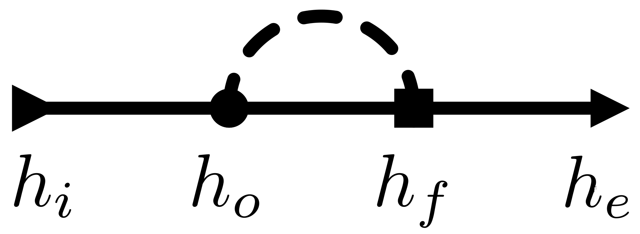
In this section, we describe our proposed model. Do keep in mind that we build it upon the concepts and terminology detailed in the previous section. In addition, we must make clear that our proposal stems from the idea of ‘unfolding’ a metaheuristic into a heuristic sequence found by solving the MCOP with a selection perturbative hyper-heuristic. What does ‘unfolding’ mean? Please take a look at Figure 1 where a metaheuristic is depicted in terms of simple heuristics (cf. Definition 8). Notice the feedback path (dashed stroke) in the metaheuristic diagram. The finaliser controls this path (cf. Definition 4). For each step, it either returns to the search operator ($h_o$) or concludes the procedure, leading to $h_e$. The signal-flow representation of metaheuristics is detailed in [7].

Now, consider a problem with a limited computational budget, which is common in real-world applications. In this case, the finaliser only anticipates the loop exit when an additional condition is met, e.g., a fitness value threshold. Nevertheless, if the finaliser role is delegated to a superior controller (say, an automated designer), we can unfold the metaheuristic scheme as a heuristic sequence. The reason: said controller not only decides when to stop applying a search operator but also which one (from a pool of search operators or heuristic space) to apply next. 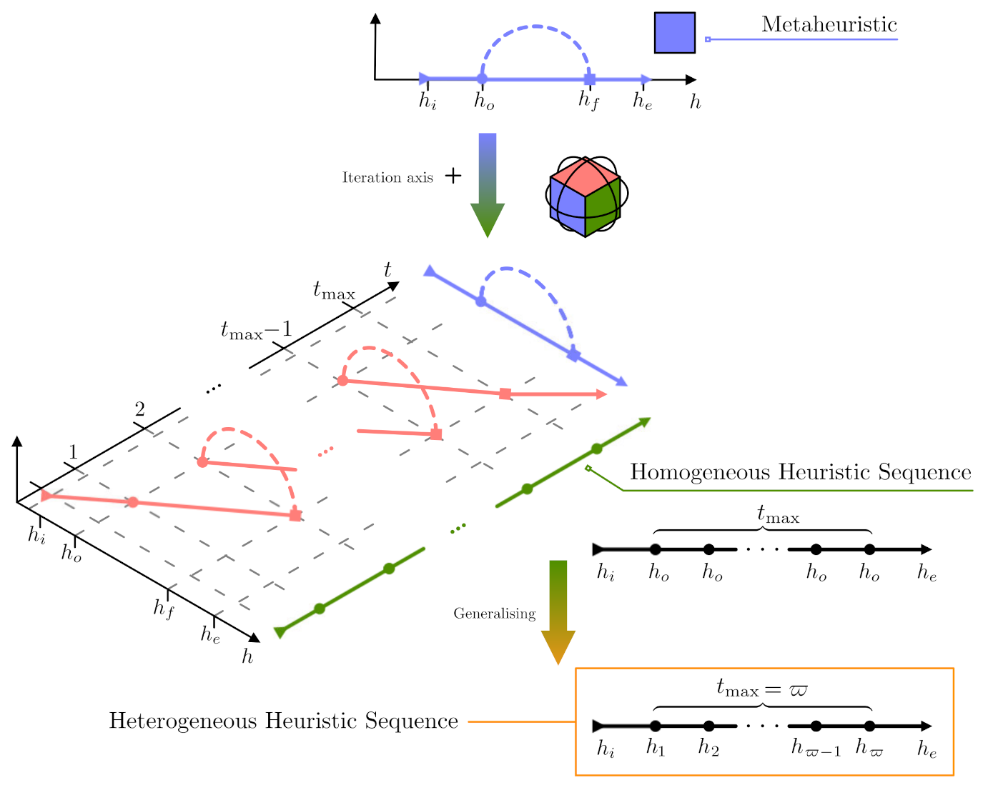Figure 2 illustrates this idea in a simple chronological plot from top to bottom. This figure also renders the signal-flow diagram of the MH with an additional axis: the time or number of iterations. We included a dummy z axis for illustrative purposes; thus, the diagram is presented with a three-dimensional perspective (check the thumbnail cube with faces coloured according to the curves). Thus, Figure 2 depicts the unfolding timeline where the signal-flow diagram of a standard metaheuristic (bluish curves) is transformed into a homogeneous heuristic sequence (greenish curves). Note that this intermediate step in the timeline corresponds to a sequence of t implementations of the same search operator ($h_o$) over the population. This can also be considered as a heuristic sequence, although a trivial one. For that reason, we labelled it as a homogeneous heuristic sequence to avoid confusion. Subsequently, it is quite natural to think about not using the same operator over and over, so we can move to a more general sequence of different (non-exclusive) search operators. This signal-flow diagram at the bottom of Figure 2 displays a heterogeneous heuristic sequence (orangish box). We called it an unfolded metaheuristic (uMH). It is worth remarking that shorter sequences are desirable, as long as they preserve the performance level. Therefore, our proposed unfolded metaheuristic model can be framed into the MCOP described in Section 2.3. Beware that, in this case, the MCOP is targeted at solving continuous optimisation problems at the lowest level of abstraction.

4. Methodology

For this manuscript, we used Python 3.7 and a Dell Inc. PowerEdge R840 Rack Server with 16 Intel Xeon Gold 5122 CPUs @ 3.60 GHz, 125 GB RAM, and CentOS Linux release 7.6.1810-64 bit system for running our experiments. Moreover, we employed the framework CUSTOMHyS v1.0 to test the proposed model with ease. This open-access framework can be found at https://github.com/jcrvz/customhys, accessed on 10 May 2021, and it is documented in [31]. Thus, we needed to specify two domains at different levels of abstraction for testing and implementing the idea.

Table 1. Description of the domains utilised in this work according to their level of abstraction and role. PF and SV stand Population-based Fixed-dimension and Single-agent Variable-dimension heuristics.

		Role
		Solver	Problem
Level of abstraction	High	Search Space: PF Heuristics, $H_{PF}\subseteq {\mathfrak{H}}^3$ Individual: Metaheuristic, ${\mathrm{MH}}_o\triangleq \langle {\eta }_i,{\eta }_o,{\eta }_f\rangle \in H_{SV}$ Procedure: $({\eta }_f\left({\eta }_o\right)\circ {\eta }_i)\left\{(H_{PF},Q)\right\}$	Domain: Heuristics, $H_{PF}\subseteq {\mathfrak{H}}^{\varpi }$ Individual: Sequence, $\overrightarrow{h}={(h_1,\dots ,h_{\varpi })}^{⊺}\in H_{PF}$ Image: $Q\left(\overrightarrow{h}\right|\mathfrak{X}):H\times \mathfrak{X}\mapsto \mathbb{R}$ Objective: Maximisation, ${max}_{\overrightarrow{h}}Q\left(\overrightarrow{h}\right|\mathfrak{X},f)$
	Low	Search Space: Continuous, $\mathfrak{X}\subseteq {\mathbb{R}}^D$ Individual: Unfolded metaheuristic, $\overrightarrow{h}={(h_1,\dots ,h_{\varpi })}^{⊺}\in H_{PF}$ Procedure: $(h_{\varpi }\circ \dots \circ h_1)\left\{(\mathfrak{X},f)\right\}$	Domain: Continuous, $\mathfrak{X}\subseteq {\mathbb{R}}^D$ Individual: Position, $\overrightarrow{x}={(x_1,\dots ,x_D)}^{⊺}\in \mathfrak{X}$ Image: Cost function, $f\left(\overrightarrow{x}\right):\mathfrak{X}\mapsto \mathbb{R}$ Objective: Minimisation, ${min}_{\overrightarrow{x}}f\left(\overrightarrow{x}\right)$

illustrates these domains, as well as their level of abstraction and role. The symbols and terminology from this table follow those from previous sections. Plus, each domain is detailed below.

At the lowest level, we selected a total of 107 benchmark functions as continuous optimisation problem domains. We considered a different number of dimensions D such as 2, 5, 10, 20, 30, 40, and 50. Plus, we categorised these problems by using their qualitative characteristics such as differentiability and unimodality in four duads of binary-encoded features, i.e., DU. With this information, we followed three manners of grouping the functions for analysing the obtained results. First, we regarded the whole set of functions, i.e., without discriminating categories, for procuring an overview of the behaviour. Then, we studied the functions grouped by feature duads: DU equals 11 (Differentiable and Unimodal problems), 10, 01, and 00 (Non-differentiable and Multimodal problems). Third, we performed a similar procedure as before, but only considering a marginal grouping, i.e., differentiability or unimodality. For example, we got differentiable and not differentiable problems neglecting the unimodality feature; a similar case applies for marginalising unimodality.

At the highest level, we utilised the population-based heuristics provided by CUSTOMHyS and also included others based on single-agent operations. Both collections belong to the heuristic space and are employed from a metaheuristic point of view. Although, the former is specialised population-based operations over a continuous problem domain with a fixed dimensionality, say, Population-based Fixed-dimension (PF) heuristics. Otherwise, the latter set corresponds to the single-agent operations, sometimes called actions, applied over a domain with variable dimensionality, say, Single-agent Variable-dimension (SV) heuristics. In this work, this particular domain is discrete, and the dimensionality is aliased to cardinality. These two sets of operators are closely related to the MCOP that we solved.  

Table 2. Ten widespread metaheuristics segregated into their search operators. Parameter data are selected based on customary values from the literature.

Type	Simple Heuristic	Variation Parameters *	Tuning Parameters
SV Perturbation	Add	–	$i\sim \mathcal{U}\{1,\varpi +1\}$
	Add Many	–	$\vartheta \sim \mathcal{U}\{1,{\varpi }_u-\varpi \}$
	Remove	–	$i\sim \mathcal{U}\{1,\varpi \}$
	Remove Many	–	$\vartheta \sim \mathcal{U}\{1,\varpi -{\varpi }_l\}$
	Shift	–	$i\sim \mathcal{U}\{1,\varpi \}$
	Shift Locally	–	$\epsilon \in {\mathbb{R}}_{++}$, $\mathcal{D}:\mathfrak{S}\times \mathfrak{S}\mapsto {\mathbb{R}}_{+}$
	Swap	–	$i,j\sim \mathcal{U}\{1,\varpi \}$
	Restart	–	–
	Mirror	–	–
	Roll	–	–
	Roll Many	–	$k\sim \mathcal{U}\{1,\varpi -1\}$
PF Perturbation	Random Sample (RX) †	$\overrightarrow{r}\ni r_i\sim \mathcal{U}(-1,1)$	$\alpha \in [0,1]$
	Random Search (RS)	$\overrightarrow{r}\ni r_i\sim \mathcal{U}(-1,1)$	$\alpha \in [0,1]$
	Local Random Walk (RW)	$\overrightarrow{r}\ni r_i\sim \mathcal{U}(0,1)$	$\alpha \in [0,1]$, $p\in [0,1]$
	Random Flight (RF)	$\overrightarrow{r}\ni r_i\sim \mathcal{L}\left(1.5\right)$	$\alpha \in [0,1]$
	Genetic Crossover (GC)	Pairing scheme, ‡ Crossover mechanism§	$m_p\in [0,1]$
	Genetic Mutation (GM)	$\overrightarrow{r}\ni r_i\sim \mathcal{U}(-1,1)$	$\alpha \in [0,1]$, $p_e\in [0,1]$, $p_m\in [0,1]$
	Differential Mutation (DM)	Mutation scheme	$M\in \{1,2,3\}$, ${\alpha }_m\in [0,3]\forall m\in \{0,M\}$
	Particle Swarm Dynamic (PS)	Velocity approach, ${\overrightarrow{r}}_i\ni r_{i,j}\sim \mathcal{U}(0,1)\forall i\in \{1,2\}$	${\alpha }_0\in [0,1]$, ${\varphi }_1,{\varphi }_2\in [0,4]$, $\kappa \in [0,1]$
	Firefly Dynamic (FD)	$\overrightarrow{r}\ni r_i\sim \mathcal{U}(-0.5,0.5)$	${\alpha }_0,{\alpha }_1\in [0,1]$, ${\alpha }_2\in [0,1000]$
	Spiral Dynamic (SD)	–	$r_0\in [0,1]$, $\theta \in [0^{\circ },{360}^{\circ }]$, ${\sigma }_r\in [0,1]$
	Central Force (CF)	–	${\alpha }_0,{\alpha }_1\in [0,0.01]$,${\alpha }_2\in [1,2]$
	Gravitational Search (GS)	–	${\alpha }_0\in [0,1]$, ${\alpha }_1\in [0,0.1]$
Selection	Direct	–	–
	Greedy	–	–
	Probabilistic	–	$p_s\in [0,1]$
	Metropolis	–	$k_B\in {\mathbb{R}}_{+}$, $\mathsf{\Theta }\left(t\right):Z_{+}\mapsto {\mathbb{R}}_{+}$

* An alternative distribution function can be implemented instead of the default one, for example, the uniform $\mathcal{U}(0,1)$, normal standard $\mathcal{N}(0,1)$, and symmetric Lévy stable $\mathcal{L}\left(1.5\right)$ ones. ^† This simple heuristic is also used as initialiser. ^‡ Available schema: random, rank weighting, roulette wheel, and tournament pairing. Tournament pairing requires two additional parameters such as $M_T\in \{1,2,3\}$ and $p_T\in ]0,1]$. ^§ Possible mechanisms: single-point, two-points, uniform, blend, and linear crossover. Linear crossover requires two additional parameters such as ${\beta }_1,{\beta }_2\in \mathbb{R}$.

summarises the simple heuristics collected for this work, and further details are provided in Appendix A. We divided them into three groups: SV perturbation, PF perturbation, and selection heuristics as aforementioned. The SV perturbators were designed conforming several works reported in the literature [32,33]. They were extracted from ten well-known metaheuristics: Random Search [34], Simulated Annelaing [35], Genetic Algorithm [36], Cuckoo Search [37], Differential Evolution [38], Particle Swarm Optimisation [39], Firefly Algorithm [40], Stochastic Spiral Optimisaiton Algorithm [41], Central Force Optimisation [42], and  Gravitational Search Algorithm [43]. We also included the random sample because it is the most straightforward manner of performing a search in an arbitrary domain. This simple heuristic also serves as the initialiser in all the implemented heuristic sequences. In this table, we present the name, variation parameters, and tuning parameters of these simple heuristics. The variation parameters concern those that drastically alter the nature of the operator. Meanwhile, tuning parameters hone the searching process. Besides, we also obtained the selectors from the metaheuristics mentioned above. It is worth mentioning that we also dedicated some words in Appendix A for documenting the finalisers commonly utilised in MH implementation.

Since we have described the problem and solution domains, we can now specify how they were employed to study the proposed model. Recall that we are studying ‘unfolded’ metaheuristics (uMHs) represented by heterogeneous heuristic sequences (cf. Figure 2). Thus, the number of iterations $t_{\max }$ is given by the sequence length or cardinality $\varpi$, i.e.,  $t_{\max }=\varpi$. In detail, we planned the experiments using a population size (N) of 30 for each unfolded metaheuristic with two cardinality limits. The first cardinality range is between 1 and 100, and the second one between 1 and 500. We selected these values to analyse the influence over the performance of a tight or a loose imposition in the sequence length. Due to this, we allowed SOs to appear more than once in the sequence. Thus, for controlling the actions that search over the heuristic space, we implemented the well-known Simulated Annealing (SA) using the Single-agent SV heuristics documented in Table 2 and Appendix A.2.1. Particularly, we utilised an initial dimensionless temperature (${\mathsf{\Theta }}_0$) of 1.0, a minimal dimensionless temperature (${\mathsf{\Theta }}_{\min }$) of ${10}^{-6}$, and a cooling rate ($\delta$) of ${10}^{-3}$. A maximal number of steps ($s_{\max }$) of 200 was set for ${\varpi }_{\max }=100$, and 500 steps were allowed for ${\varpi }_{\max }=500$. We refer henceforth to these two configurations as Experiments 1 and 2, respectively. Subsequently, to assess the performance of each uMH (say, $\overrightarrow{h}$) when solving a given problem, we ran each candidate $N_r=50$ times and recorded the last fitness values. Then, we estimated its performance using

$$Q(\overrightarrow{h})\approx -(\mathrm{med}+\mathrm{iqr})(\{\forall {\overrightarrow{x}}_{\ast ,r}\in X_{\ast }|f({\overrightarrow{x}}_{\ast ,r})\}),$$

(5)

where med and iqr are the median and interquartile range operators, respectively, applied to the fitness values $f\left({\overrightarrow{x}}_{\ast ,r}\right)$. The symbol ‘≈’ indicates that the estimation depends on the $N_r$ samples $X_{\ast }$ obtained from a stochastic process. Plus, the minus sign in (5) is because HH deals with a maximisation problem (cf. Definition 9), but the objective function $f\left(\overrightarrow{x}\right)$, at the low-level domain, corresponds to a minimisation problem (cf. Definition 1). We chose this formula mainly because the median and the interquartile range are better descriptors in the presence of outliers. We also based this selection on several a priori results from previous works [31,44]. Lastly, and for the sake of clarity, we summarised the procedures performed for each problem in Pseudocode 1. In this, we refer to the SV heuristics as actions when they are described along with the PF heuristics to avoid confusion.

Pseudocode 1: Hyper-heuristic based on Simulated Annealing (SAHH)

Input:  Domain x, objective function f, heuristic collections HPF, HSV (cf. Table 2), initialiser hi, performance $Q\left(\overrightarrow{h}\right|\mathfrak{X},f)$, and popula1tion size N. Additional parameters: $\mathsf{\Theta },{\mathsf{\Theta }}_{\min }$ and δ. Output:  Best heuristic secquence h∗ 1: $\overrightarrow{h}\leftarrow$ ChooseRandomly ($H_{PF}$, $P_{H_{PF}}$) ▹$P_{H_{PF}}\left(h\right)$ is the probability distribution of $H_{PF}$ 2: for $r=\{1,\dots ,N_r\}$do     ▹ Repeat the subsequent evaluations $N_r$ times 3:   $X_{\ast }\ni {\overrightarrow{x}}_{r,\ast }\leftarrow$ EvaluateMH$\overrightarrow{h}$  ▹ Evaluate and record the candidate sequence 4: end for 5: $\mathrm{perf}\left(\overrightarrow{h}\right)\leftarrow Q\left(\overrightarrow{h}\right|\mathfrak{X},f)$ via Equation (5)    ▹ Estimate the performance metric 6: ${\overrightarrow{h}}_{\ast }\leftarrow \overrightarrow{h}$                  ▹ Initialise the best heuristic sequence 7: $s\leftarrow 0$, and $\mathsf{\Theta }\leftarrow {\mathsf{\Theta }}_0$           ▹ Initialise the step counter and temperature 8: while$\left(\mathsf{\Theta }>{\mathsf{\Theta }}_{\min }\right)$ and $(s\le s_{\max })$ do 9:  $a\leftarrow$ ChooseAction$H_{SV},a,\varpi$ ▹ Choose an action at random from the action set $a\in H_{SV}$ 10:  ${\overrightarrow{h}}_c\leftarrow a\left\{\overrightarrow{h}\right\}$    ▹ Obtain a neighbour sequence ${\overrightarrow{h}}_c$ by applying a to $\overrightarrow{h}$ 11:  for $r=\{1,\dots ,N_r\}$ do   ▹ Repeat the subsequent evaluations $N_r$ times 12:   $X_{\ast }\ni {\overrightarrow{x}}_{r,\ast }\leftarrow$ EvaluateSequence${\overrightarrow{h}}_c$ ▹ Evaluate and record the candidate sequence 13:  end for 14:  $\mathrm{perf}\left({\overrightarrow{h}}_c\right)\leftarrow Q\left({\overrightarrow{h}}_c\right|\mathfrak{X},f)$ via Equation (5)  ▹ Estimate the performance metric 15:  if $\mathcal{U}(0,1)\le exp(-(\mathrm{perf}\left({\overrightarrow{h}}_c\right)-\mathrm{perf}\left({\overrightarrow{h}}_c\right))/\mathsf{\Theta })$ then  ▹ Apply Metropolis selection 16:   $\overrightarrow{h},\mathrm{perf}\left(\overrightarrow{h}\right)\leftarrow {\overrightarrow{h}}_c,\mathrm{perf}\left({\overrightarrow{h}}_c\right)$ 17:  end if 18:  if $\mathrm{perf}\left({\overrightarrow{h}}_c\right)<\mathrm{perf}\left({\overrightarrow{h}}_{\ast }\right)$ then                  ▹ Apply Greedy selection 19:   ${\overrightarrow{h}}_{\ast },\mathrm{perf}\left({\overrightarrow{h}}_{\ast }\right)\leftarrow {\overrightarrow{h}}_c,\mathrm{perf}\left({\overrightarrow{h}}_c\right)$, and $s\leftarrow 0$ 20:  else 21:   $s\leftarrow s+1$ 22:  end if 23:  $\mathsf{\Theta }\leftarrow \mathsf{\Theta }(1-\delta )$                        ▹ Decrease the temperature 24:  end while 24:   25: procedure EvaluateSequence$\overrightarrow{h}$ ▹ Apply the composition: $(h_{\varpi }\circ \dots \circ h_1\circ h_i)\left\{\mathfrak{X}\right\}$ 26:  $t\leftarrow 0$ 27:  $X\left(t\right)\ni {\overrightarrow{x}}_n\left(t\right)\leftarrow h_i\left\{\mathfrak{X}\right\},\forall n\in \{1,\dots ,N\}$          ▹ Initialise the population 28:  $F\left(t\right)\ni f_n\left(t\right)\leftarrow f\left({\overrightarrow{x}}_n\left(t\right)\right),\forall n\in \{1,\dots ,N\}$        ▹ Evaluate the population 29:  ${\overrightarrow{x}}_{\ast }\left(t\right)\leftarrow {\overrightarrow{x}}_k\left(t\right)$ since $k=arginf\left\{F\right(t\left)\right\}$  ▹ Find the best global position by Direct selection 30:  for $t=\{1,\dots ,\varpi \}$ do                        ▹$t_{\max }=\varpi =\#\overrightarrow{h}$ 31:   $h_{p,t},h_{s,t}\leftarrow h_t\in \overrightarrow{h}$  ▹ Read the perturbator and selector from the t-th search operator 32:   $X\left(t\right),F\left(t\right)\leftarrow h_{p,t}\left\{X\left(t\right)\right\}$                ▹ Apply the t-th perturbator 33:   ${\overrightarrow{x}}_{\ast }\left(t\right)\leftarrow h_{s,t}\left\{X\left(t\right)\right\}$  ▹ Update the best global position using the t-th selector 34:  end for 35:  return ${\overrightarrow{x}}_{\ast }\left(t\right)$ 36: end procedure

5. Results and Discussion

After carrying out the experiments described in the previous section, we study all the results using different approaches to validate our proposal. These approaches are organised as we now mention. We first discuss some punctual implementations to detail the unfolded metaheuristics designed by the SAHH approach. Then, we study the number of iterations from both low- and high-level approaches. They are the metaheuristic cardinality $\varpi$ (or the number of search operators) and the hyper-heuristic steps s. Later, we discuss the nature of those operators selected by SAHH to be part of the customised uMHs. Right after analysing these characteristics, we evaluate the performance of the overall approach and the individual unfolded metaheuristics. Finally, we focus our attention on the time complexity of the methodologies that comprise this research.

5.1. Illustrative Selected Problems

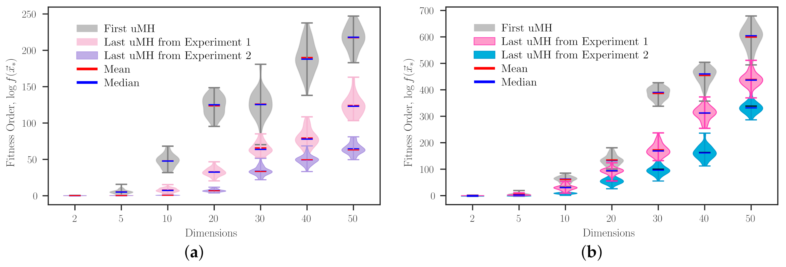
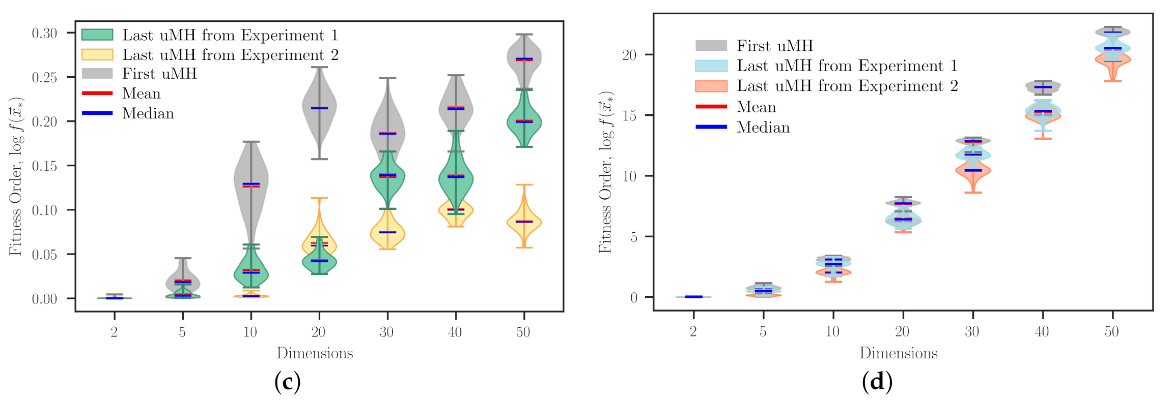
First of all, we selected a problem from each category to illustrate the implementation of the proposed approach. Figure 3 shows how the SAHH procedure improves the heuristic sequence that it initially picked at random. To enhance the readability of these data, we plotted fitness order values, which were calculated using logarithm base 10 $logf\left({\overrightarrow{x}}_{\ast }\right)$, instead of the bare fitness values. Note that each violin in this figure corresponds to a heuristic sequence, where light-grey violins stand for the initial candidate sequence. In contrast, coloured ones correspond to those obtained from each experiment. In all the plots, the influence of the dimensionality over the problem domain is quite observable. This is expected, considering the established conditions (same population size and maximal cardinality). Regarding the maximal cardinality, it is straightforward to infer that unfolded metaheuristics (uMH) obtained from Experiment 2, which has a loose cardinality range, generally improve upon the corresponding uMHs from Experiment 1. An exception of this general improvement, which may not be the only one, can be seen when solving the problem Type I (Figure 3) with 20 dimensions. However, when the number of dimensions equals 50 for the same problem, it is easy to notice a remarkable difference between the two resulting metaheuristics. However, this does not imply that one achieved uMH is better than the others. Recall that each experiment has different conditions, and the resulting methodologies have distinctive properties, e.g., the type and the number of search operators (SOs) composing them. Nevertheless, an objective fact noticed at a glance from Figure 3 is the relatively compact shape of uMHs from Experiment 2. This is to be expected, chiefly because they were designed to have more SOs than those from Experiment 1. Thus, in raw words, they had more opportunities to ‘refine’ their search procedure. It is also worth remarking that even considering one design specification or the other, employing a particular approach may not grant a relevant benefit when dealing with some problems with exceptional ‘hardness’. An example of that can be observed in Figure 3d, where the uMHs tailored for the non-differentiable and multimodal (DU = 00) Schaffer N3 problem exhibit similar performances, close to that of the first uMH guessed by SAHH.

Table 3. Illustrative results from the selected problems in Figure 3. Columns correspond to the problem name, its binary-encoded category (DU), the achieved performance metric value (Perf.), unfolded metaheuristic cardinality ($\varpi$), and hyper-heuristic steps (s). Better performances are in bold face.

Problem	DU	Dim.	Experiment 1			Experiment 2
			Perf.	$\mathit{\varpi }$	s	Perf.	$\mathit{\varpi }$	s
Schwefel	11	2	0.001	67	129	6.2$\times {\mathbf{10}}^{-\mathbf{4}}$	494	323
		5	0.402	99	189	0.050	226	421
		10	11.025	100	187	0.669	483	216
		20	38.686	99	158	8.475	498	465
		30	74.324	94	180	37.957	499	273
		40	89.752	99	164	55.137	498	288
		50	137.846	90	99	70.506	499	441
Rastrigin	10	2	0.001	82	40	3.9$\times {\mathbf{10}}^{-\mathbf{9}}$	378	72
		5	3.413	96	118	1.405	498	190
		10	40.683	100	142	14.999	500	180
		20	105.712	92	74	69.849	500	360
		30	196.954	89	192	117.694	266	380
		40	341.164	100	175	194.557	465	345
		50	463.786	94	162	358.056	490	404
Type I	01	2	1.3$\times {10}^{-4}$	68	24	1.1$\times {\mathbf{10}}^{-\mathbf{5}}$	311	127
		5	0.008	100	45	6.1$\times {\mathbf{10}}^{-\mathbf{4}}$	500	203
		10	0.046	89	164	3.6$\times {\mathbf{10}}^{-\mathbf{3}}$	499	145
		20	0.053	100	187	0.074	473	15
		30	0.155	99	15	0.087	499	491
		40	0.155	100	170	0.109	497	464
		50	0.214	87	20	0.094	497	392
Schaffer N3	00	2	0.004	100	108	1.6$\times {\mathbf{10}}^{-\mathbf{3}}$	377	44
		5	0.657	97	78	0.236	483	247
		10	3.005	73	110	2.305	496	318
		20	6.989	87	190	6.578	471	455
		30	12.253	97	43	11.029	495	310
		40	15.862	94	170	15.697	500	202
		50	20.992	77	60	20.093	497	158

complements the results from Figure 3. Concerning the performance value, it is evident that Experiment 2 promotes reaching better performing unfolded metaheuristics for most cases. However, this is not a general rule. An exception is observed in the performance value of the uMH designed for the 20-dimensional Type I problem (Figure 3). This is self-explained by remembering that SA is just a single-agent metaheuristic implemented as an HH. We have not run several implementations of the same HH problem as we did for evaluating the heuristic sequences because it exhibits a high computing cost. For this work, we employed SAHH as a well-established (stochastic) approach to design uMHs by solving the MCOP, which is considered ill-posed due to the presence of multiple solutions. Bear in mind that if there exists a unique solution, the NFL theorem is violated. This is an interesting discussion that is beyond our scope. Furthermore, it is worth noticing that there are some cases where quite similar performances can be rendered from dramatically different heuristic sequences, for example, those achieved for the Schaffer N3 problem with $D\ge 10$. In that case, it is preferable to use the setup from Experiment 1 or to enhance the HH solver. Plus, we can observe with ease that, on average, Experiment 1 and 2 obtained 92- and 460-cardinality uMHs, in HH procedures with an average of 121 and 283 steps, respectively. In terms of search operators, both implementations achieve methods close to the upper limit, but that was not the case of the required hyper-heuristic steps, at least in this illustrative example. A relevant fact to highlight from these data is the apparent absence of a cardinality ($\varpi$) and the increasing trend of heuristic steps (s) related to the dimensionality. It seems that our approach somehow deals with the dimensionality curse when solving the MCOP. However, this occurs at the high level, where this parameter can be considered as a design condition.

5.2. Low- and High-Level Iterations

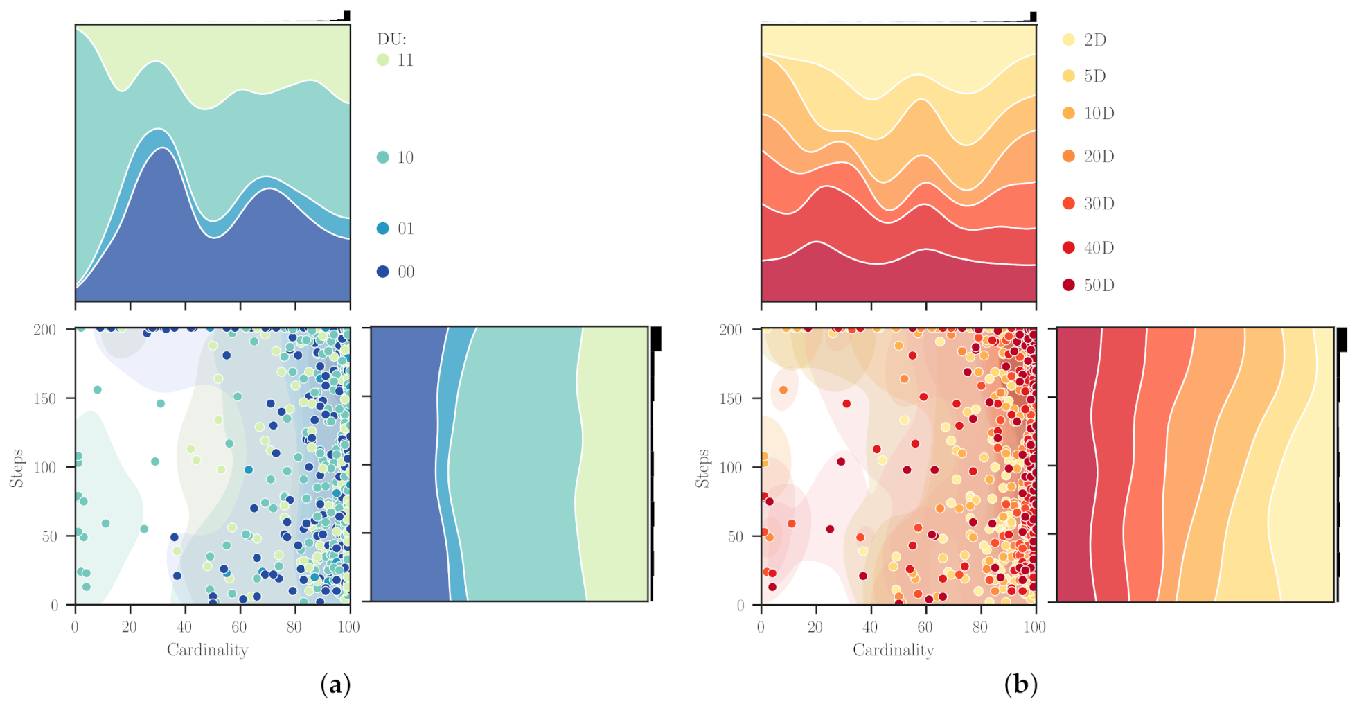
After taking a smooth dive into the results using some punctual examples, we now analyse them from different perspectives. Figure 4 shows the normalised distribution of steps and cardinality when grouping this information by using the categories (DU) and the number of dimensions. It is pretty evident that for both parameters, $\varpi$ and s, the maximal concurrence is near the upper limit (see the distributions in the margins of the diagonal plots). In this case, we used all the results obtained from Experiment 1, but one can notice a somewhat similar pattern from Experiment 2. From Figure 4a, we observe that uMHs with $\varpi$ of about 30 (followed by 70) were more frequently designed for non-differentiable problems. At the same time, for the differentiable one, the cardinalities were more scattered along with the domain. Particularly, it is interesting that our approach found several ‘short’ heuristic sequences with up to 20 search operators for differentiable and multimodal (DU = 10) domains. This is remarkable because short procedures would be preferred in many practical implementations. Now, concerning the steps spent finding these uMHs, the distributions show relatively uniform shapes along with the limits. Using a different lens, Figure 4b, we encountered some inferences about $\varpi$ and s when grouping the results by problem dimensionality. In general, it is worth noting the presence of two modes for the cardinality, near 30 and 70, when the two-dimensional problems are considered. Increasing dimensionality seems to slightly shift these modes to 20 and 60 when search domains reach 50 dimensions. This is an unexpected behaviour that can only be attributed to the capabilities of the proposed approach for dealing with high-dimensional problems. Plus, some particular facts to mention are as follows: for 5D domains, there are no low cardinalities; for 10D and 20D, uMHs of about 40 search operators are less frequent; and for 30D, the $\varpi$ distribution is weighted to its extrema. Lastly, by looking at the steps required to design these metaheuristics, we can remark an evident transition from s values loaded about the first half of the studied range (i.e., from 1 to 100) for the 2D problems to a uniform-like distribution for those with 50D. In addition, it is somewhat understandable that for lower-dimensional domains, the hyper-heuristic implementation of Simulated Annealing required ‘few’ steps for finding an optimal heuristic sequence. In such cases, we know the problem hardness is mainly related to its inherent characteristics, and the influence of the dimensionality curse is not so relevant. The following analysis is intended to attain more information about this discussion.  

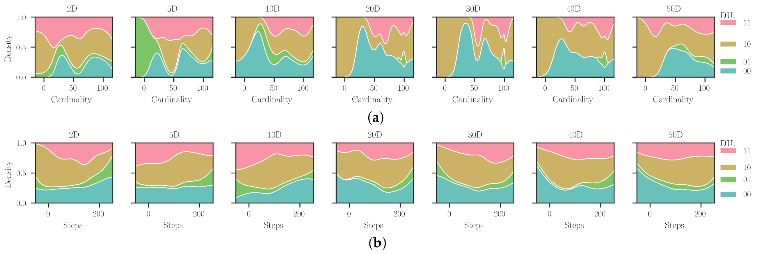
Figure 5 extends the results from Figure 4 by combining the dimensionalities and categories for distributions of both metaheuristic and hyper-heuristic iterations (i.e., cardinality and steps, respectively). Figure 5a shows that uMHs with more than 25 search operators are more prevalent when solving problems with extreme combinations of DU, i.e., 11 and 00. Although, there is an exception for each category. For the differentiable and unimodal problems, it appears when their dimensionality equals two, which is somewhat expected due to their inherent ‘simplicity’. For the non-differentiable and multimodal problems, one can notice low cardinality uMHs can be attributed to the SAHH solving procedure and other parameters worth studying in future works. Besides, $\varpi$ distributions found for uMHs solving differentiable and multimodal functions are diverse and range almost every value for all dimensions. It is crucial to notice that for this category (DU = 10), our approach managed to find unfolded metaheuristics with up to 50 search operators with a remarkable frequency. The remaining category, non-differentiable and unimodal problems, renders quite interesting patterns, most of them showing compact distributions about the 100-cardinality uMHs. We may remark that this behaviour is chiefly led by the fact that such a characteristic combination is a bit unusual, so there are few problems within this category (DU = 10). In particular, our collection comprises 26, 45, 8, and 28 problems for the DU categories 11, 10, 01, and 00. Furthermore, Figure 5b exhibits the steps required by the hyper-heuristic to find a proper uMH for solving a problem from a given category and dimensionality. These distributions are, by far, smoother than those for the cardinality, which is somehow understandable because they belong to a higher level of abstraction (indirectly related to the problem domain). Except for the two-dimensional case, the steps required by SAHH to find the uMHs vary from a distribution that is highly concentrated in the lower limit into one akin to a uniform distribution. Again, we can explain the particular behaviour for 2D because most of the candidate heuristic sequences during the HH procedure were worth considering. Using an analogy with the Law of Supply and Demand, we could state that there is more supply than demand. For the intermediate categories (say, 10 and 01), a slight transition from left- to right-hand loaded distributions is observable. Thus, dimensionality seems to directly influence the number of steps required for designing a solver that deals with problems from these categorical features. Lastly, for the non-differentiable and multimodal problems, we notice a reversed pattern with respect to distributions from the differentiable and unimodal problems. It is quite interesting to see how our approach manages to find uMHs for these functions using few steps with more frequency.

5.3. Nature of Search Operators

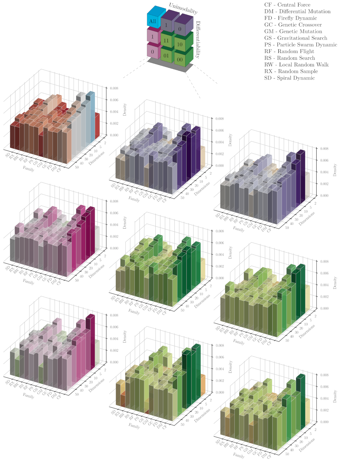
By this point, we have analysed the influence of categories and dimensionality in the unfolded metaheuristic cardinality and the required hyper-heuristic steps. Now, we delve into the nature of the search operators, particularly the perturbators, conforming these uMHs achieved via Experiment 1. We also disregard a detailed analysis from Experiment 2 due to their similarities with this case. Figure 6 presents bidimensional histograms involving the operator families employed in the metaheuristics for solving problem domains with different dimensionalities. We believe that Figure 6 is quite illustrative about the manner we perform this classification (see the thumbnail blocks in the upper centre). In the first block (upper-left corner), we observe the family distributions for ‘All’ the problems without considering their categorical features. We split all these results using the categorical characteristics, unimodality and differentiability, as we did above. The purple and magenta plots in the first row and column, respectively, correspond to the marginal cases where only one feature is considered, i.e., only differentiability (right blocks) or unimodality (bottom blocks). Greenish plots show the results for particular combinations of the differentiability and unimodality characteristics in a matrix-shape form. In general, we notice that our approach manages to deal with a given problem with certain conditions (characteristics and dimensionality) by arranging operators from one family or another to build its solver. There are some situations where a family is often preferred from others, as we discuss below. Nevertheless, it does not mean that a particular set of operators is the best for such a situation. We are just showing the nature of those operators selected for conforming an unfolded metaheuristic found throughout a hyper-heuristic search.

From the histogram for all the functions in Figure 6, it is easy to notice that operators from the Genetic Crossover (GC) and Random Search (RS) families were more frequently selected for dealing with two-dimensional problems. This fact is somehow expected due to the ‘simplicity’ of these problems where, in general, a simple stochastic approach would be enough to solve them. Obviously, GC is not such a simple approach, but we believe that its unstructured outcomes with respect to the other operators explain this behaviour. For greater dimensionalities, perturbators from the Central Force (CF) family became more relevant, but it seems to be attenuated when augmenting the number of dimensions. A similar effect is noticed with the GC perturbators and, slightly different, with the RS ones that show an increase in popularity around five and ten dimensions. On the contrary, we found that simple heuristics from Gravitational Search (GS) and Particle Swarm (PS) families seem, in a more notorious way, to be boosted up when dimensionality rises. One may explain such a fact with the ‘swarm’ interaction of the probes representing such operators, making them more suitable for higher-dimensional problems. Regarding the family distribution per dimension, we must remark that this becomes more uniform when increasing the problem dimensionality. Nevertheless, we note that mutation-based operators (from Genetic and Differential Mutation families) are oft-chosen to build heuristic sequences for solving 50-dimensional problems.

In general, the shape observed for the overall case, without categories, is preserved when grouping the results as mentioned. To better scrutinise these family distributions, the following lines are dedicated to remark those interesting situations that appear when grouping the results. For non-differentiable problems, operators based on random walks (e.g., RS) seem to be invariant in popularity, with a high-density value, concerning the dimensionality. This effect can be observed in detail at the blocks corresponding to categories 10 and 00. Likewise, the Gravitational Search (GS) family appears to be invariant to dimensionality and exhibits low-density values. This is also noticed in a reduced proportion for the Spiral Dynamic (SD) family. We can notice that GS heuristics start as the less popular ones when dealing with 2D domains for the marginally differentiable problems. Still, they gradually increase in density to a moderate value when the 50D problems are considered. This behaviour is also regarded in the block of marginally multimodal problems. It is crucial to remark that we observe a more uniform density distribution with respect to dimensions and families for this marginal classification. Nevertheless, it is quite obvious that this is mostly inherited from the differentiable and multimodal problems (DU = 10).

5.4. Performance Analysis

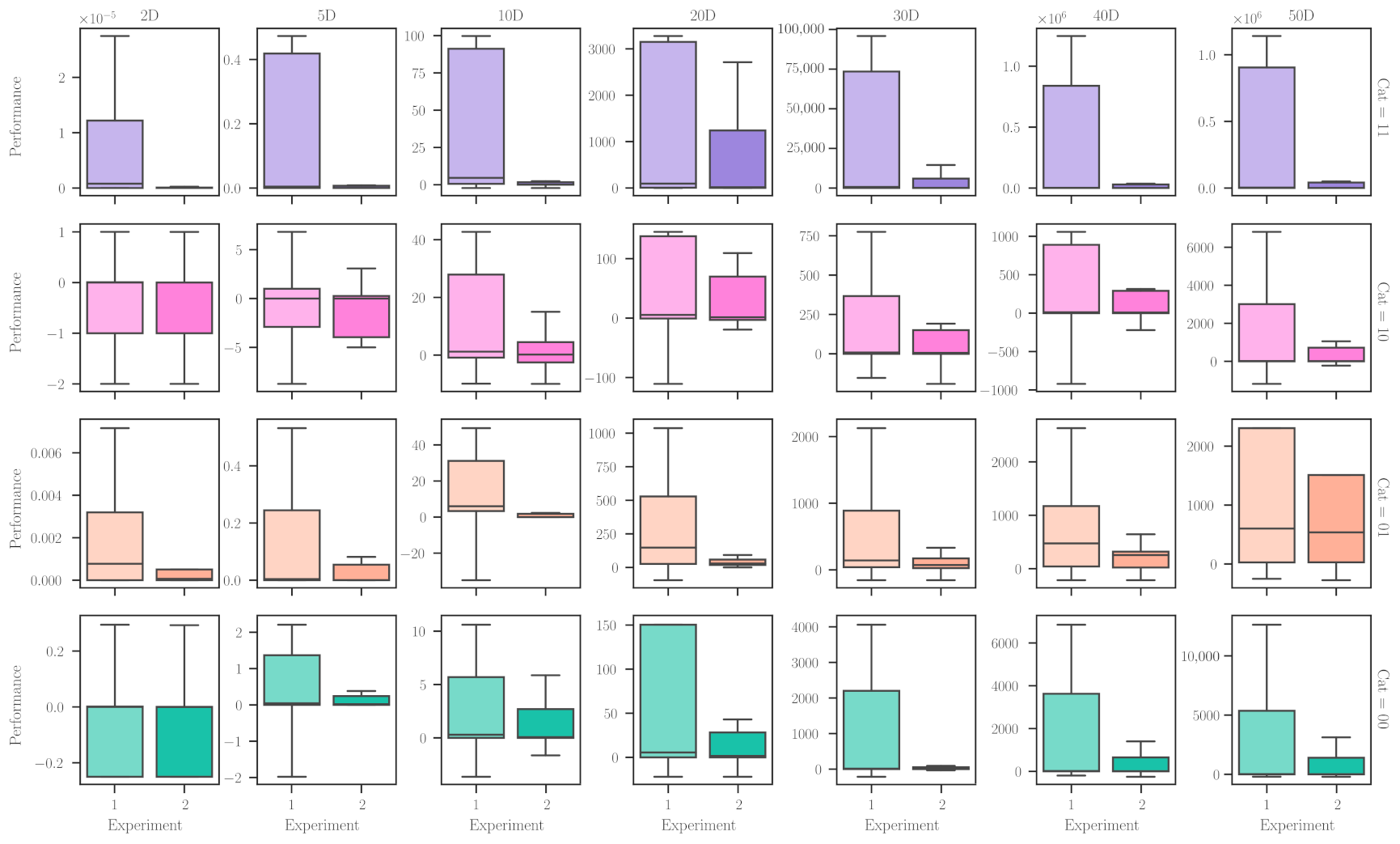
Once we have boarded the cardinality, required steps, and nature of the resulting unfolded metaheuristics, which are somehow similar for the two experimental setups, we proceed to study the most crucial feature of them: performance. Figure 7 presents the performance values for the resulting uMHs from the two experimental setups, when solving the problem domains with different characteristics and dimensionalities. In this figure, rows correspond to the combination of problem categories (differentiability and unimodality), and columns are the number of dimensions. It is pretty easy to notice that the conditions of Experiment 2 promote better performing uMHs than those of Experiment 1. Nevertheless, this is not a general rule. For example, when dealing with multimodal problem domains (say, DU = 10 and 00), the performance distribution for both experimental setups is virtually the same in the context of boxplots. One can explain such a fact with the dimensionality of these problems, making them ‘easy’ to solve. Naturally, if we have to choose a procedure to find an adequate solver, we would prefer to implement Experiment 1 because it requires fewer resources. In the other cases, it is evident that those additional requirements render notably better performing metaheuristics. Another point to emphasise is the precision of these performance values, with Experiment 2 allowing more concentrated values than the other.

For our subsequent discussion, we compare the achieved unfolded metaheuristics against the collection of basic metaheuristics, which are also provided by the CUSTOMHyS framework [31], using the same performance metric. These basic methods are those used for extracting the simple heuristics but implemented with different default hyper-parameters. This gives us a total of 66 MHs. The first comparison is also the most straightforward: performance-to-performance. Thus, we calculated the Success Rate (SR) for an achieved unfolded metaheuristic (uMH) for a given problem domain $(\mathfrak{X},f)$ compared against ($M=66$) basic MHs implemented in the same domain, such as,

$$\mathrm{SR}\left(\mathrm{uMH}\right)\triangleq \frac{1}{M}\sum _{i=1}^{M}H\left(Q\left(\mathrm{uMH}|\mathfrak{X},f\right)-Q\left({\mathrm{MH}}_i|\mathfrak{X},f\right)\right),$$

(6)

where $H:{\mathbb{R}}^D\to {\mathbb{Z}}_2^D$ is the Heaviside step function and $Q\left(\overrightarrow{h}\right|\mathfrak{X},f)$ is the performance metric from (5). SR means a weighted counting of how many basic MHs were beaten (outperformed) by the designed uMH per problem and dimensionality. Although analysing the individual SR for each problem domain cannot be insightful, we aggregated the SR values from problems sharing the same category and dimensionality employing the average operation. Thus, we obtained an Average Success Rate (ASR) measurement that Figure 8 shows. With that in mind, we must notice that our approach, whichever experimental configuration, surmounts the performance of at least one basic metaheuristic in almost all problems (i.e.,  $\mathrm{ASR}>0$). This is crucial because even for an excellent solver for a given problem, we must know its limitations and advantages. However, employing the approach we are proposing in this manuscript, we as practitioners are able to find automatically a heuristic-based solver for any problem. It may not be the best one, but it is a good starting point for further enhancements. 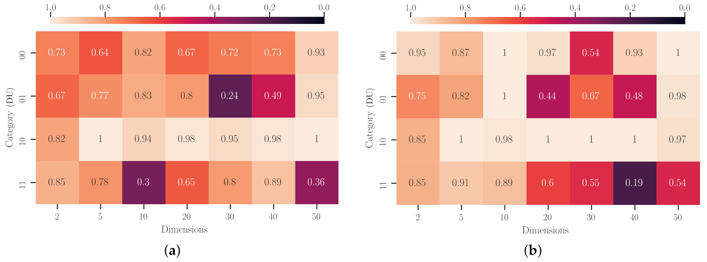These words are supported with the non-zero values of ASR that Figure 8 depicts; it means that the uMH achieved by SAHH has beaten at least one basic MH. Moreover, we must emphasise that ASRs from Experiment 1 were, in general, improved when we implemented the second setup. The most notorious scenarios where our approach surmounts the basic metaheuristics are the multimodal (DU = 10 and 00) problems. On the contrary, unimodal problem domains seem to be difficult rims, paradoxically, due to their ‘easiness’, for tackling these basic metaheuristics. In other words, the relatively low success rates do not imply that our approach has trouble solving these problems. It just means that many basic MHs can achieve good performance values.

Subsequently, we analyse the results by carrying out multiple comparisons using the pairwise (one-sided) Wilcoxon signed-rank test. Thus, we compute the true statistical significance for multiple pairwise comparisons such as $p=1-{\prod }_i(1-p_i)$ by following the procedure and conditions given in [45,46]. We employed the performance value reached by the metaheuristics, for each problem and dimension via (5), as the measure of one run of the algorithm. Thus, we set the unfolded metaheuristic generated by SAHH as the control parameter and the basic metaheuristics as the other parameters. We look for the statistical significance of uMHs outperforming at least one of the basic MHs in a given problem. In doing so, we justify the fact that we do not require prior knowledge of which problems a particular MH is an excellent choice. Keeping this in mind, we state the null and alternative hypotheses as:

Hypothesis 0.

(Null) The unfolded metaheuristic, generated by the SAHH approach, performs equal to or worse than at least one basic metaheuristic with a significance level $0.05$.

Hypothesis 1.

(Alternative) The unfolded metaheuristic, generated by the SAHH approach, outperforms at least one basic metaheuristic with a significance level of $0.05$.

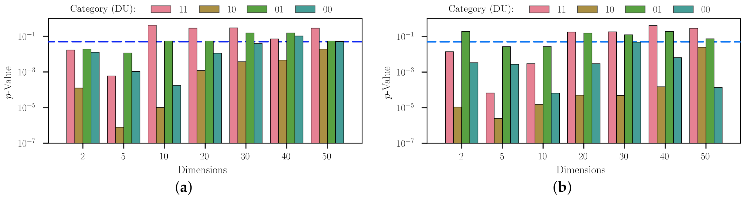
Figure 9 shows the p-values from this Wilcoxon’s analysis, and also grouped by category and dimensionality. At a general glance, we notice that it is possible ($p<0.05$) to reject the null hypothesis H${}_0$ for several scenarios in both experimental setups. Particularly, for those liaised with the multimodal domains, numerous basic metaheuristics are not suitable for dealing with them. It is also worth mentioning that the number of dimensions seems to increment the p-values determined for these scenarios. Nevertheless, it does not mean that SAHH generates poor-performing unfolded metaheuristics. We attribute this tendency to fail to reject the null hypothesis because these problems become harder to solve with any technique. It is also valuable to comment that Experiment 2 represents a better configuration than Experiment 1 for most problems with a dimensionality beyond five. On the opposite side, we can find those problem domains with a unimodal landscape where it is hard to find a method incapable of solving them. Likewise, increasing the dimensionality has a similar effect as the one we just commented. However, we only fail to reject H${}_0$ when regarding the nondifferentiable and unimodal problems in 2D and Experiment 2. This result is quite understandable because this setup proffers to generate longer heuristic sequences from longer HH searching procedures. It may also be considered a drawback of using a memoryless metaheuristic approach to deal with a hyper-heuristic problem. Naturally, if the practitioner decides to apply our approach for low-dimensional problems, we highly recommended a configuration similar to Experiment 1. Otherwise, Experiment 2 would suffice as a good starting point for dealing with more than twenty dimensions.

5.5. Time Complexity Analysis

All the terms mentioned below follow the nomenclature described in Section 2 and Section 3. After analysing the nature of the resulting heterogeneous heuristic sequences, we are interested in studying the computing cost of our proposal. Keep in mind that once a uMH is designed for any problem, its implementation or further tuning for a relatively similar problem requires a low computing burden; it could be even lower than that required for a standard metaheuristic. Thus, we only focus our attention on the hyper-heuristic process for designing these uMHs. In that sense, SAHH has a time complexity similar to that of a regular metaheuristic, given by

$$\begin{array}{cc}\hfill T_{\mathrm{SAHH}}& =T_{\tilde{p}}+T_{\tilde{f}}+T_{\tilde{s}}+s_{\max }\ast (T_{\tilde{p}}+T_{\tilde{f}}+T_{\tilde{s}})\hfill \\ \hfill & =\mathcal{O}\left(s_{\max }\ast sup\left\{T_{\tilde{p}},T_{\tilde{f}},T_{\tilde{s}})\right\}\right),\hfill \end{array}$$

(7)

since $T_{\tilde{p}}$, $T_{\tilde{f}}$, and $T_{\tilde{s}}$ are also the computational costs of evaluating the perturbator, objective function, and the selector, respectively; and $s_{\max }$ is the maximal number of steps carried out in this high-level search. Plus, SAHH is a single-agent algorithm, so selection, perturbation, and acceptance are actions considered to have constant time, i.e.,  $T_{\tilde{p}}=T_{\tilde{s}}=\mathcal{O}\left(1\right)$. Otherwise, the objective function at this high level stands for the performance metric described in (5), so its computing cost is given by $T_{\tilde{f}}=\mathcal{O}\left(N_r\ast T_{\mathrm{uMH}}\right)$, where $N_r$ is the number of repetitions, and $T_{\mathrm{uMH}}$ is the cost of implementing a candidate uMH. Naturally, the time for calculating the median and interquartile range is disregarded due to its magnitude. In summary, we can rewrite the SAHH time complexity as

$$T_{\mathrm{SAHH}}=\mathcal{O}\left(N_r\ast s_{\max }\ast T_{\mathrm{uMH}}\right).$$

(8)

Now, regarding the low level, the time complexity for an unfolded metaheuristic composed of up to ${\varpi }_{\max }$ search operators yields

$$T_{\mathrm{uMH}}=\mathcal{O}\left({\varpi }_{\max }\ast N\ast D\ast T_p\right),$$

(9)

since N is the population size, D is the dimensionality, and $T_p$ is the computational cost of evaluating the perturbator. According to the well-known Big-$\mathcal{O}$ definition, this value can be determined such as $T_p=sup\{T_{p,1},\dots ,T_{p,\varpi }\}$ for the uMH. It is easy to notice that the initialiser, finaliser, and selectors have an irrelevant complexity contribution. Besides, we focus on analysing the procedure and not the problem to solve, so we can adopt without loss of generality that the time complexity of evaluating the fitness is constant. Equation (9) can be employed to find the theoretical time complexity of any unfolded metaheuristic for some given conditions, for example, Experiments 1 or 2. In that case, we must use the worst case for $T_p$; i.e., $T_p=\mathcal{O}\left(N^2\right)$ for the Genetic Crossover perturbator with Cost-based Roulette Wheel Pairing [47]. Thus, uMHs have a cubic time complexity with respect to the population size and a linear one with respect to the dimensionality, which is relatively high but affordable considering the context of designing solvers.

Keeping this in mind, we can express the time complexity of the overall approach $T_{\mathrm{SAHH}}$ by plugging (9) in (8), as shown,

$$T_{\mathrm{SAHH}}=\mathcal{O}\left(N_r\ast s_{\max }\ast {\varpi }_{\max }\ast D\ast N^3\right).$$

(10)

This expression gives us information about which components influence the time complexity of the overall approach. Notice that we considered the maximal number of search operators ${\varpi }_{\max }$ instead of $\varpi$, which can be different from one uMH to another. From the above analysis, it is exciting to surmise that the running time scales linearly with the problem dimensionality and cubically with the population size; which is somehow manageable. The main reason is the high-level metaheuristic (i.e., SAHH) controlling the process, which performs one modification per step in a single element of the unfolded metaheuristic. For the scope of this research, SAHH constitutes a good prospect with a low computational burden.

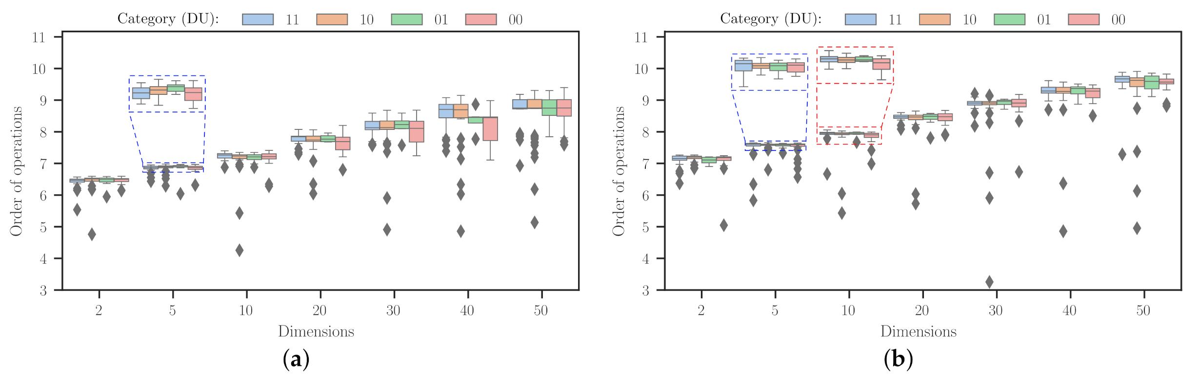
Furthermore, we can use (9) to assess the order of operations required by the designed uMHs to tackle problems with different characteristics and dimensionalities. Thus, instead of the overall worst case of $\mathcal{O}({\varpi }_{\max }\ast T_p)$, we approximated this by accumulating the number of operations done for each simple heuristic from the uMH achieved in the SAHH procedure, i.e., $\mathcal{O}({\varpi }_{\max }\ast T_p)\approx {\sum }_{k=1}^{\varpi }{T}_{p,k}$. Figure 10 displays this information as boxplots, where the effect of the problem dimensionality is evident for both experimental setups. First, it is interesting to note that Experiment 2 allows for more search steps, promoting a more refined heuristic sequence that solves a given problem. Such a fact translates into operation values more concentrated around a specific amount. This has meaningful implications in providing more confidence to the practitioner when implementing the approach proposed in this work. Although, it is not a secret that using this setup instead of the first one would have an additional computing burden. Plus, it is worth mentioning that the order of operations does not increment too dramatically, as we foresaw with the brief theoretical analysis. Likewise, as we expected, the difference between Experiments 1 and 2 (Figure 10a,b, respectively) does not constitute an abyss. Indeed, the overall value is 0.74 ± 0.41 with a mean value of 0.70. This is due to the low computational burden that SA imposes on the HH approach. The second setup has 300 and 400 units more in $s_{\max }$ and ${\varpi }_{\max }$ than those for the first setup. In general, we must notice that results for non-differentiable and unimodal functions represent the most expensive procedure for both experimental setups. It is also remarkable that many of the outliers from Figure 10 are mostly situated at data liaised with differentiable (DU = 11 and 10) problems. This is an unusual combination of characteristics since problems from this category exhibit diverse behaviours. Such a fact must be a matter to be considered in further works.

6. Conclusions

This work proposed a new heuristic-based solver model for continuous optimisation problems. However, our proposal can be easily extended to other domains. Such a model, which we named ‘unfolded’ metaheuristic (uMH), comprises a heterogeneous sequence of simple heuristics. This is achieved by delegating the control mechanism in the standard metaheuristic scheme to a high-level strategy. Hence, this implies solving the Metaheuristic Composition Optimisation Problem (MCOP) to tailor a particular uMH that tackles a specific optimisation problem. We carried out a proof-of-concept by utilising the CUSTOMHyS framework, which is publicly available at https://github.com/jcrvz/customhys, accessed on 10 May 2021. Through CUSTOMHyS we analyse 107 continuous optimisation problems and a collection of 12 population-based fixed-dimension heuristics, extracted from ten well-known metaheuristics in the literature, to search in the problem domain. Thus, we specified the unfolded metaheuristic model and implemented a Hyper-Heuristic (HH) based on Simulated Annealing (SA), SAHH in short, to solve the MCOPs. For the SAHH, we also incorporated 11 single-agent variable-dimension heuristics to search in the heuristic domain. We considered two main experimental setups. The first one allowed uMHs of up to 100 search operators, with SAHH performing up to 200 steps. The second one considered up to 500 operators and steps. In the manuscript, we refer to the number of search operators in a uMH as its cardinality, $\varpi$.

From the results, we found that our proposed approach represents a very reliable alternative, with low computing cost, for designing optimisation population-based metaheuristics that solve continuous problems. To complement this claim, we shortly summarise several insights extracted from the experiments we carried out. First, we noticed that SAHH manages to find an unfolded metaheuristic, which deals with the optimisation problem, no matter the imposed design conditions. Naturally, some conditions affect the performance of the outcoming solvers. For example, the cardinality range does not directly affect the uMH performance, but when this range is relaxed, the uMH commonly renders more precise performance values. However, this has the drawback of increasing time complexity (or the number of operations) as a trade-off for a greater chance of balanced exploration and exploitation features. Besides, we found some leads indicating that the dimensionality affects the metaheuristic and hyper-heuristic iterations (i.e., cardinality and steps, respectively) on a scale related to the problem characteristics. The influence of dimensionality over problem hardness acts like a catalyst that amplifies the inherent difficulty given by its characteristics. In such cases, we noted that uMHs with greater cardinality only slightly outperform those with lower $\varpi$ values, so we must recommend using the low-cost ones in practical implementations. Nevertheless, we have not detected an abysmal difference between the unfolded metaheuristics obtained from the studied setups in the number of operations, i.e., about 0.70 of the median value. This is a great feature due to the heuristic nature of the solvers that our approach generates.

We also studied the nature of the search operators that are automatically selected by SAHH when building uMHs. We remark that SAHH often chooses operators from the Genetic Crossover and Random Search families for two-dimensional problems. However, their frequency seems to be attenuated when increasing the number of dimensions. A similar case was observed with simple heuristics of the Central Force nature, but starting with 5D problems and an evident greater dominance. Conversely, we regard operators from the Gravitational Search and Particle Swarm families correspond to the less frequent ones at the 2D mark, although they become relevant during the dimensionality increment. We attribute this effect to the nature of these families, related to multi-probes intelligent interactions, which performs better on broader search domains. In the end, for the greatest dimensionality, we observed a pretty uniform distribution from almost all the families of search operators. Therefore, we infer that operators slightly sophisticated to the random ones are enough to fulfil the solver requirement for few dimensions. More nature-diverse operators are needed for many variables.

Lastly, we carried out a similar experiment using the metaheuristics selected for extracting the search operators used to construct the heuristic space employed by SAHH; we called them basic MHs. We found that our uMHs surmount the average performance of at least one basic metaheuristic for the same problem domain. Such a fact has a tremendous repercussion in the context of the No-Free-Lunch (NFL) theorem, mainly because the practitioner does not have to know which is the excellent metaheuristic for a given problem. Instead, s/he only has to use our approach, and it will indeed find a good one with some particular requirements. Bear in mind that this work does not pretend to violate the NFL theorem. Instead, we are using it in our favour to propose suitable solvers.

To the best of our knowledge, this unfolded metaheuristic model has not been previously proposed in the literature. According to our results, it is a model worth considering in practical implementations because it seems to be a very reliable and low-cost computing approach for solving optimisation problems. We know that our model is not a panacea. There are several issues to deal with for further understanding and improvement; some are now commented. To alleviate the influence of dimensionality and problem characteristics, we plan to loosen the constraints imposed on the cardinality and steps, and include other relevant parameters, such as the population size. In the same way, we believe that improving the hyper-heuristic algorithm (i.e., SAHH) must increase the overall performance of the resulting uMHs. An alternative and faster approach requires considering a non-heuristic-based algorithm such as a Machine Learning methodology. Plus, we are going to consider additional benchmark problems, including those utilised in algorithm competitions, e.g., CEC and GECCO. Lastly, we plan to implement this approach in a practical engineering scenario to test its feasibility to achieve low-budget heuristic sequences. We considered it a relevant topic for future works.