Abstract
In this study, singular integral solutions were studied to investigate scattering of Rayleigh waves by subsurface cracks. Defining a wave scattering model by objects, such as cracks, still can be quite a challenge. The model’s analytical solution uses five different numerical integration methods: (1) the Gauss–Legendre quadrature, (2) the Gauss–Chebyshev quadrature, (3) the Gauss–Jacobi quadrature, (4) the Gauss–Hermite quadrature and (5) the Gauss–Laguerre quadrature. The study also provides an efficient dynamic finite element analysis to demonstrate the viability of the wave scattering model with an optimized model configuration for wave separation. The obtained analytical solutions are verified with displacement variation curves from the computational simulation by defining the correlation of the results. A novel, verified model, is proposed to provide variations in the backward and forward scattered surface wave displacements calculated by different frequencies and geometrical crack parameters. The analytical model can be solved by the Gauss–Legendre quadrature method, which shows the significantly correlated displacement variation with the FE simulation result. Ultimately, the reliable analytic model can provide an efficient approach to solving the parametric relationship of wave scattering.
1. Introduction
The propagation of disturbances known as wave propagation in solids has been studied in many branches of physical science and engineering. Wave propagation carries energy (e.g., kinetic and potential energies) through a solid medium and energy transmission over a radiation pattern is through the motion of particles in the wave motion phenomenon. Although wave motion in elastic solids is well-studied, adequately defining a wave scattering model by objects such as cracks still can be quite a challenge.
Over the past decades, crack evaluations using a wave scattering approach in nondestructive evaluations (NDEs) have gained much attention [1,2]. Many researchers in the early 1980s offered analytical solutions to define and explain the scattered surface waves caused by cracks (e.g., subsurface cracks) [3,4,5]. A vertical subsurface crack is considered capable of generating an efficiently scattered field since the crack is one of the most influential damages of surface wave propagation. The analytical model of a vertical subsurface crack [3] is obtained by establishing an integral representation for the scattered field expressed in terms of the fundamental potentials first introduced by Lapwood [6]. Furthermore, numerical methods have been devised to solve the singular integral equations of the analytical model. For example, the Gauss–Chebyshev quadrature rule as a numerical method was adopted by Erdogan and Gupta [7]. Understanding the numerical solution of a singular integration is vital to providing an accurate and reliable solution to the analytical wave scattering model. Such studies have focused on scattered wave motions presented in relation to the displacement variations caused by different frequencies and geometrical crack parameters. Based on this approach, a well-defined relationship can be developed to evaluate causes and estimate behavioral patterns in cracks. Although using the relationship between displacement variations and frequencies can lead to evaluate cracks by solving the inverse problem, research is needed to verify displacement variations in the existing analytical solutions.
Meanwhile, high-performance computers and simulation software have facilitated efficient wave modeling studies [8,9], which perform with experimental studies under the constraints of time, environment, sources, etc. Several methods have been conducted to simulate the mechanical wave propagation in solid mediums. Among them, finite element (FE) simulation is widely used for higher accuracy and adaptability. Hassan and Veronesi [8] performed a comparative study of FE simulation of wave propagation and laser interferometry experiment with a cracked steel plate to show the reliability of FE simulation. FE results allow simulation of waveform change between the incident wave and scattered wave based on the resultant crack(s). One challenge of FE simulation of wave propagation is that it requires a large-sized simulation model to avoid wave reflection at the model’s boundary. Furthermore, the model should have enough distance between the wave source and listening nodes to obtain pure waveforms (e.g., surface wave). Typically, a minimized model has been designed to streamline computational efficiency. Oh and his colleagues [10] conducted practical FE simulations using a damper and energy-absorbing element known as an infinite element to minimize the model size. They proposed a combination of damper and infinite element with a required absorbing thickness and damping factor, so dampers could prevent wave reflection.
Both analytical and simulation methods (e.g., FE) are powerful approaches for wave modeling, which aim to predict or provide a specific parametric relationship in a system (e.g., variations of a scattered wave amplitude by different frequencies and crack sizes). The simulation method is beneficial when a complex wave model is needed (e.g., complicated geometry and various incident waves). In addition, an analytical model has applicability limitations needing corrections of some factors (e.g., nonlinearity, wave amplitude-dependent) [11,12]. However, an analytical method is still a powerful approach to calculate the wave model needs rapidity to provide computational efficiency. This is especially true when the simulation model has become too time-consuming and requires heavy computations. Thus, use of a reliable analytical model can significantly save efforts and provide an efficient approach to solving the parametric relationship of wave scattering. Furthermore, beyond the computational benefit, an analytical method is helpful in understanding the fundamental wave propagation through a mathematical formulation that is derived from wave motion and elastodynamic theory [13].
In this study, we investigate the existing analytical model of the displacement variations of scattered surface waves, and study different numerical integration methods for the proposed analytical model. We also introduce an efficient dynamic FE analysis to demonstrate the viability of the wave scattering model with an optimized model configuration for wave separation. Finally, we verify the analytical model with the FE simulation results uniquely. To solve the singular integral equations in the analytical model, five different numerical integration methods of Gaussian quadrature were considered: the Legendre quadrature (GLEQ), the Gauss–Chebyshev quadrature (GCQ), the Gauss–Jacobi quadrature (GJQ), the Gauss–Hermite quadrature (GHQ) and the Gauss–Laguerre quadrature (GLAQ). The obtained displacement variation curves from the analytical models are compared and verified with FE simulation results by defining the correlation of the curves.
2. Analytical Model
The analytical model of the wave scattering is defined in Section 2. The aim of the theoretical model is to calculate the displacement variation subject to the crack geometry and incident wave frequencies in a homogeneous, isotropic and linearly elastic solid medium on the half-plane condition defined as the set of points (x, y) in the Cartesian plane with . The subsurface crack is formed, as shown in Figure 1, with varying a and b parameters.
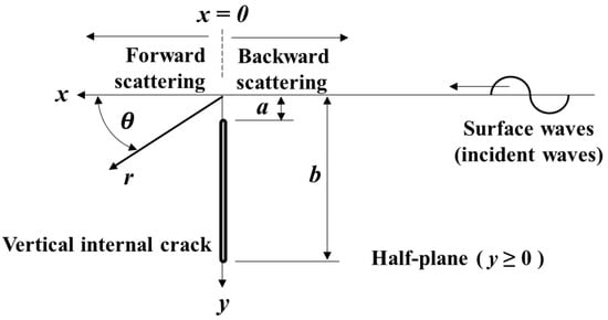
Figure 1.
Illustration of subsurface crack on the two-dimensional half-plane. is the distance between the ground and the top of the crack tip, is the distance between the ground and the bottom of the crack tip and and are components of the polar coordinate. The image shows the directions of the incident waves and scattered waves influenced by different and distances.
2.1. Derivation of Displacement Potentials.
The displacement field as the final theoretical model can be expressed as two potential functions, a scalar potential and a vector potential by Helmholtz decomposition [14]:
where is the displacement field of scattered waves and is the Nabla or Del operator. Computing the displacement potentials is the main part of defining the theoretical scattering model. The displacement field is defined in the -invariant condition. The waves in the half-plane are z-invariant waves where all functions are dependent on the z-direction. The displacement potentials are defined in the scattered field and satisfy a radiation condition of the elliptic boundary-value problem by Wickham [15] as the equation including the exponential and small ‘’ functions:
where and are constant; , and are the Rayleigh wavenumbers, longitudinal waves and transverse waves, respectively. and are the components of the polar coordinate (, ). The signs denote forward direction, + and backward direction, . The part including the polar coordinate in the Equation (2) is ignored since the incident wave angle is 90 degrees. The coefficient and satisfy the equation and are given as:
The constant can be obtained by Equation (3) when the constant can be calculated as an explicit formula given Achenbach’s approach [16], which can be expressed as:
Where
The components of integration in Equation (4) are given as:
where, and are the displacement functions in y-direction and x-direction, respectively. The displacement functions can be obtained by Hooke’s law, , where is a displacement matrix, is a force matrix and is a stiffness matrix. The force matrix can be computed by the stress field given by Achenbach [3] as:
where is Poisson’s ratio.
The stiffness matrix is obtained by the equations representing the Hankel function, which is a Bessel function of the third kind.
where is the third order of the first kind of Hankel function, is the first order of the first kind of Hankel function and
where is a density and is a digamma function of a complex variable obtained by differentiating the logarithm of a gamma function.
2.2. Numerical Integral Solutions of an Analytical Model
The ultimate objective of this study is to calculate and verify displacement variations, which is defined by the ratio of displacements as scattered wave and incident wave occurrences. The displacements are calculated from the potentials derived by the singular integral Equation (4) Notably, numerical integration methods are key to solve the analytical model to provide reliable and accurate displacement variation. Five Gaussian quadrature numerical integration methods are employed: GLEQ, GCQ, GJQ, GHQ and GLAQ.
The key to the Gaussian quadrature method is to define the node (x) and weight (w), which is the additional coefficient known as “weight” at the element and given by the weight function, to calculate integration in numerically as described in Equation (12). The rule of integration is stated as
where is a continuous function, is a dependent variable at a discrete node and is the weight function at the discrete node .
To define the node or the reference point in the x coordinate, an orthogonal polynomial is utilized. Depending on the applied orthogonal polynomial, the five numerical integration methods are classified. The Gauss–Legendre quadrature is the simplest integration problem by Legendre polynomials on [−1, 1], and the weight function is:
where is the Legendre polynomial, which is the solution of the Legendre differential equation .
The Gauss–Chebyshev quadrature uses Chebyshev polynomials with respect to the weight function, which is given as:
The Gauss–Jacobi quadrature is for an approximate integral with the Jacobi polynomials and weight function expressed as:
where f is a smooth function on [−1, 1] and α, β > −1. The interval [−1, 1] can be replaced by any other interval by a linear transformation. The Gauss–Hermite quadrature is a form of Gaussian quadrature for approximating the value of integrals of the following kind, and the weight function is given as:
where is a Hermite polynomial, which is the solution to Hermite’s differential equation, .
The Gauss–Laguerre quadrature is an extension of the Gaussian quadrature method for approximating the value of integrals for the following kind and the weight function is:
where is the Laguerre polynomial, which gives the solution to Laguerre’s equation of a second-order linear differential equation, . Weight functions of each numerical integration method are described in Table 1.

Table 1.
Weight function of integral methods.
3. Computational Simulations Model
The computational simulations, especially the finite element (FE) analysis, is the most widely used method to solve field problems using a numerical approach. In this study, the FE modeling is performed to verify analytical models solved with different numerical integral methods. The model will simulate the wave propagation in the solid media, including the vertical subsurface crack with different frequencies of incident waves. In detail, the cracks are designed by the different ‘’ values and ratios. Three values of the parameter ‘’ to simulate subsurface crack in those depths are 12 mm, 18 mm and 24 mm cracks, as denoted in Table 2. The selected parameters are typical sizes in the field area. In addition, two ratios with 0.1 and 0.2 are considered to design the internal crack. The increase in the ratio indicates the decrease in crack sizes. These ratios are selected to compare with the existing analytical solution [3]. In addition, the proposed analytical model will be verified with the FE simulation. Each case has a different wavenumber range. A total of 177 FE models are simulated. A total of 150 FE models are designed for 6 different crack geometry cases simulated varying different frequency ranges. For example, there are 27 models for C12–0.1 case for simulating different frequencies described in Table 2. Twenty-seven FE models out of 177 are designed for no crack case.
Table 2.
Designed crack geometry and simulation numbers by the wavenumber range.
3.1. Model Description
Typically, an FE simulation requires a large-sized simulation model to avoid unexpected waves reflected from the boundary; otherwise, it will show considerable computation time. Several researchers [10] have conducted the FE simulation with damper and energy-absorbing elements (i.e., infinite elements) to reduce the size of the model. The study of FE simulation with damper and infinite element recommends 10 damping zones in an 0.4–0.6/length (distance between wave source and boundary) with 1000 to 2000 of step damping factor increase. Since the simulation model of this study has a shorter distance between the wave source and boundary, 1000 of the initial damping factor, and 5000 of the incremental damping factor are chosen. The FE models in this study compose of three groups: the solid medium group, damper group and wave absorbing infinite element group. The solid medium size is 4000 mm (width) 1000 mm (height). The 500 mm damper zone is at the boundary of the solid medium group and is represented in the rainbow color of Figure 2. The infinite element is placed at the dampers’ end. The applied material properties are assumed for the typical solid material ( = 2400 kg/m2, E = 35 GPa and = 0.2), which is the largest component in the model. Both the analytical model and the FE model have applicability limitations for typical material cases having material nonlinearities that may affect wave propagation. We assume linear elastic wave propagation. The explicit FE simulation does not enforce the structural equilibrium [17], therefore the structural boundary condition is not necessary for the structural equilibrium of the internal structure forces under the external load. The model of the ABAQUS solver is designed using a two-dimensional (2-D) four-node plane strain element (CPE4R) with 2 mm mesh size for the solid medium group and dampers.
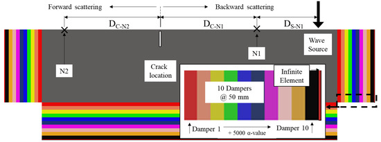
Figure 2.
Details of finite element (FE) model: is the listening node for the backward scattered waves, is the listening node for the forward scattered waves, and are the distances between the crack and nodes, and , respectively, is the distance between the wave source and . The figure also includes ten dampers in rainbow colors on the three sides of the solid medium and an infinite element in the thin red layer at the end of dampers. The illustration shows the required component and geometry to simulate the wave propagation in the cracked model.
The artificially attenuated dampers are designed by gradually increased alpha mass-proportional damping factors, as described in Table 3. Typically, the damper zone allows attenuating low-frequency waves, while the infinite element absorbs high-frequency waves [10]. The type of the element is an infinite element, CINPE4.
Table 3.
Damping factors for optimum damping gradient of FE model.
3.2. Discussion of the Wave Separation in FE Simulation
The model based on the wave separation in the P-wave and surface waves is studied in this section. As illustrated in Figure 2, the represents a distance between the crack location and listening nodes in the x-direction, while represents the distance between the source point and backward listening node in the x-direction. Typically, each propagated wave (e.g., P-wave, S-wave and surface wave) has a different arrival time due to each wave’s different speed. For example, in the simulation with given material property, the speed of the P-wave ( and surface wave () are 4084 m/s and 2265 m/s, respectively. However, the model requires a minimum distance between the wave source and the listening nodes to obtain the pure waveforms (e.g., surface wave) so as to avoid overlapped waves.
Figure 3 shows four different wave groups excited by an incident sine wave. The two-wave groups (P-wave and surface wave) are incident waves in the time range between 0.2 and 0.8 x 10⁻³ s, while the other two-wave groups are the reflected waves at the crack in the time range between 1.2 and 1.6 x 10⁻³ s. The three following groups must be considered to obtain a clear P-wave and surface wave separation: i) Reflected P-waves by the crack should not pass when the incident surface waves pass through at , as . ii) the distance, should be enough to have a wave separation in P- and Surface-waves at , (see Region A in Figure 3), , where T is period of the incident wave. should be enough to have a wave separation between the reflected P- and Surface-waves by the crack at the and , (see region B in Figure 3), . In addition, the simulations are designed to avoid the S-wave effect to obtain the pure surface wave by receiving only the horizontal displacement, which is in a longitudinal direction, thus the S-wave was eliminated.
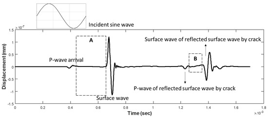
Figure 3.
FE simulation results of the time-domain waveform at the node in horizontal x-displacement: Waves from the incident wave and reflected waves by the crack are calculated. Both Region A and B show different arrival times as wave separations of the P-wave and surface waves. Region A is associated with the incident waves and B is associated with the reflected waves by crack. The image explains the waveform in the time-domain and the required distance of and to obtain a pure waveform of the surface waves.
4. Results and Discussions
The FE simulation is performed to verify the analytical model introduced in Section 2. The numerically calculated analytical model and FE simulation results are described to the displacement variation of the ratio of the backward scattered wave and incident wave, and the ratio of the forward scattered wave and incident wave by two parameters of ‘a’ and ‘’, which is related to the frequency (: k is a wavenumber, f is a frequency and C is the wave speed).
4.1. Results of the Analytical Model and FE Simulation
The analytical model with five different integral methods is computed using MATLAB (2019, MathWorks, Natick, MA, USA) in accordance with the procedures of Section 2. The FE simulation is designed based on the details described in Section 3. The analytical model and FE simulation results are normalized with the highest magnitude of the variation ratio to compare the shape and tendency of each case. The wavenumbers are considered to have the displacement variation curves in the range by the given ‘’ values (e.g., 12 mm, 18 mm and 24 mm). In the simulation result of the forward scattered case, the pure scattered waves are obtained at a higher frequency range than 10 kHz. Since the lower frequency (e.g., 10 kHz or below) has a longer wavelength, the scattered P-wave overlaps the scattered surface wave, as discussed in Section 3.2.
Figure 4 includes two graphs of the backward and forward scattered cases of the C18–0.2 model, which has a 72-mm crack size. In this geometry, the higher amplitude of scattered energy variation shows in the forward scattered direction (see the amplitude of the in Figure 4) than in the backward direction (see the amplitude of the in Figure 4).
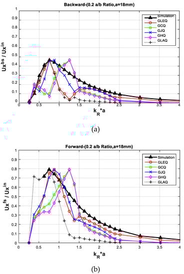
Figure 4.
Displacement variation curves from the analytical model and FE simulation by the different direction of the C18–0.2 model: (a) backward scattering and (b) forward scattering result. The curves show the shape of the displacement variation denoted as and in the analytical model and simulation result. The results indicate that the analytical models solved by different internal methods show a shape similar to that of the FE simulation in both the forward and backward case.
The displacement variation changes depending on distance between the ground and top crack, denoted as ‘’ and the crack size are described in Figure 5. The three models considered are C12–0.2, C18–0.2 and C24–0.2, which have depths of 12 mm, 18 mm and 24 mm, respectively and a crack size of 48 mm, 72 mm and 96 mm. The models have the same ratio, 0.2. Regardless of the crack depth and size, a similar amount of wave scattering occurs in the same ratio.
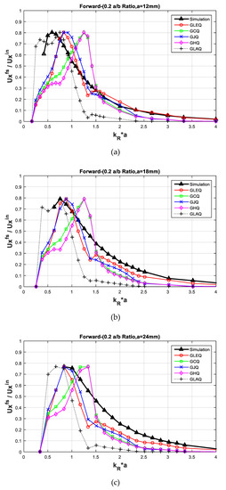
Figure 5.
Displacement variation curves of analytical model solving five different integral methods and FE simulation shown with different crack depths, ‘ ’ of the forward scattered models: (a) result with a 12 mm and a 0.2 ratio model (C12–0.2), (b) results with an 18 mm and 0.2 ratio model (C18–0.2) and (c) results with 24 mm of and a 0.2 ratio model (C24–0.2). The figure implies the deeper crack depth which is a higher ‘’ result shows the peak point at the higher value.
The displacement variations based on crack size change is described in Figure 6, including C12–0.1 and C12–0.2 case, which have a 108-mm and 48-mm crack size. The graph result showing 0.1 of the a/b ratio (see Figure 6a) is obtained by a longer crack than the 0.2 case (see Figure 6b) and the model shows a sharper triangular shape of curves in the lower value. The small crack size case has its peak value at the relatively higher . Since the lower frequency waves can pass through the smaller length or size of the crack, it shows lesser wave scattering energy in the lower . Thus, the peak displacement variation is formed in the higher as part of a smaller crack model.
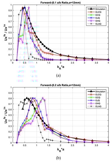
Figure 6.
Displacement variation curves of the analytical model and FE simulation by different a/b ratio of the forward scattering models: (a) result from 0.1 ratio model (C12–0.1), (b) result from 0.2 ratio model (C12–0.2). The figure implies the longer crack model represents the higher wave scattering energy and narrow distribution curve. The peak displacement variations of the shorter crack model are obtained at the relatively higher value.
4.2. Representative Correlation Values of Curves
The correlation coefficient is used for quantifying the similarity between two variables. In this study, Pearson’s correlation coefficient [18] is adopted to evaluate the similarity of the displacement variation curves. The method of Pearson’s correlation coefficient gives the coefficient () value between −1 and 1 to define the similarity of the two curves. When > 0, it means that the two variables are positively correlated and when < 0, the two variables are negatively correlated. When = 1, it means that the two variables are completely and linearly correlated, that is, they have a functional relationship. When = 0, it refers to the nonlinear correlation between the two variables. When 0 < < 1, it means there is a certain degree of linear correlation between the two variables, as described in Table 4. And, the closer is to 1, the closer the linear relationship is between two variables. If is closer to 0, the linear correlation is weaker between two variables, as described in Table 5.
Table 4.
Condition of correlation coefficient and its relationship between variables.
Table 5.
Criteria for a correlation coefficient.
The Pearson’s correlation coefficient (r) is calculated by Equation (18):
where and is the mean of variable and . In the discussion section, the results of the FE simulation will be compared with the analytical models using five different numerical integration approaches.
The calculated correlation coefficients are described in Table 6. The averages of the obtained correlation coefficients from the five integral methods range from 0.79 to 0.94. Therefore, all five integral methods are in the highly linear correlation condition in Table 5. Among the applied integration methods, the Gauss–Legendre quadrature method shows a higher correlation, e.g., 0.94 and obtained an averaged correlation coefficient.
Table 6.
Calculated correlation coefficient results between FE simulation and analytical solution by five different numerical methods; the Gauss–Legendre quadrature method (GLEQ) shows the highest similarity. GCQ: the Gauss–Chebyshev quadrature; GJQ: the Gauss–Jacobi quadrature; GHQ: the Gauss–Hermite quadrature; GLAQ: the Gauss–Laguerre quadrature.
The distance of the correlation coefficient between the analytical model and FE simulation can be explained with considerable limitations: 1) the assumption of the analytical model which is not considered in FE simulation and 2) methodological difference between the analytical solutions and FE simulation.
The analytical model is derived based on many assumptions to make the mathematical logic simple. For example, the analytical model uses Green’s function expressed in terms of the Hankel functions to obtain the stiffness function (see and in Equation (10)). Since Green’s function adopts a point source effective solution based on the Dirac delta function in mathematical terms, the analytical model limits the non-localized explicit solution. Thus, the results show a difference from the FE simulation results, which is the explicit time variable solution. In addition, the FE simulation results are affected by the distance ( and ) and incident waveform; however, the analytical model has no variables pertaining to the horizontal distance and incident waveform.
5. Conclusions
The presented study mainly focuses on singular integral solutions to investigate the existing analytical model and to provide a new analytical solution. The study also presents an efficient dynamic FE analysis with an optimized model configuration for wave separation. The simulation that uniquely offers the wave scattering phenomena is designed to obtain the displacement value under the same given conditions as with the analytical model. The data from the simulation results are used to demonstrate the viability of the wave scattering model. The obtained analytical solutions with displacement variation curves are investigated by defining the Pearson’s correlation of the FE results. Finally, the result shows the significantly correlated displacement variation of the proposed model with the FE results. The obtained results are discussed in terms of the curved shape and the correlation coefficient between the analytical model and FE simulation. The following conclusions are drawn based on the analytical solutions and FE simulation results and discussion presented in the study.
- The computation time of the analytical model is much shorter than the FE simulation. In the study, 177 FE models are created and simulated in order to provide an adequate resolution of the displacement variation curves. Each simulation computing time is about 20 minutes, and post-processing is required, while the numerical solution for analytical model takes a few seconds without designing and post-processing time.
- Regardless of crack depth and size, a similar amount of wave scattering energy occurs in the same ratio.
- The smaller crack sized model has a peak value at the relatively higher . Since the lower frequency waves can pass through the smaller length of the crack, it shows lesser wave scattering in the lower . Therefore, the peak displacement variation is formed in the higher in the case of the smaller crack model.
- The Gauss–Legendre quadrature integration method shows the highest correlation coefficient values, with an averaged value of 0.94 compared to all considered models, between its analytical model and the FE simulation.
- The analytical model can provide an efficient and reliable approach to solving the parametric relationship of wave scattering. Further studies are needed to investigate the limits of applicability of the developed analytical formulation, such as nonlinearity.
Author Contributions
S.K. and S.H. designed the study; S.K. and Y.C.W. carried out numerical simulation, analyzed the collected. S.H. acquired the funding, supervised the study, reviewed and improved the manuscript draft. All authors have read and agreed to the published version of the manuscript.
Funding
This research was funded by the U.S. Department of Transportation, Tran-SET, Grant Number 19SAUTA04 and 19SAUTA03.
Conflicts of Interest
The authors declare no conflict of interest.
References
- Ham, S.; Popovics, J.S. Application of contactless ultrasound toward automated inspection of concrete structures. Autom. Constr. 2015, 58, 155–164. [Google Scholar] [CrossRef]
- Ham, S.; Popovics, J.S. Application of micro-electro-mechanical sensors contactless NDT of concrete structures. Sensors 2015, 15, 9078–9096. [Google Scholar] [CrossRef] [PubMed]
- Achenbach, J.D.; Brind, R.J. Scattering of surface waves by a sub-surface crack. J. Sound Vib. 1981, 76, 43–56. [Google Scholar] [CrossRef]
- Achenbach, J.D.; Brind, R.J.; Norris, A. Scattering by Surface-Breaking and Sub-Surface Cracks. Proc. DARPA/AFWAL Rev. Prog. Quant. NDE 1981, 58, 340–347. [Google Scholar]
- Achenbach, J.D.; Lin, W.; Keer, L.M. Surface Waves due to Scattering by a Near-Surface Parallel Crack. IEEE Trans. Sonics Ultrason. 1983, 30, 270–276. [Google Scholar] [CrossRef]
- Lapwood, E.R. The Disturbance Due to a Line Source in a Semi-Infinite Elastic Medium. Philos. Trans. R. Soc. A Math. Phys. Eng. Sci. 1949, 242, 63–100. [Google Scholar]
- Erdogan, F.; Gupta, G.D.; Cook, T.S. Numerical solution of singular integral equations. In Methods of Analysis and Soultions of Crack Problems; Springer: Dordrecht, The Netherlands, 1973; Volume 1, pp. 368–425. [Google Scholar]
- Hassan, W.; Veronesi, W. Finite element analysis of Rayleigh wave interaction with finite-size, surface-breaking cracks. Ultrasonics 2003, 41, 41–52. [Google Scholar] [CrossRef]
- Ávila-Carrera, R.; Rodríguez-Castellanos, A.; Valle-Molina, C.; Sánchez-Sesma, F.J.; Luzón, F.; González-Flores, E. Numerical simulation of multiple scattering of P and SV waves caused by near-surface parallel cracks. Geofis. Int. 2016, 55, 275–291. [Google Scholar]
- Oh, T.; Popovics, J.S.; Ham, S.; Shin, S.W. Practical finite element based simulations of nondestructive evaluation methods for concrete. Comput. Struct. 2012, 98–99, 55–65. [Google Scholar] [CrossRef]
- Reda, H.; Karathanasopoulos, N.; Ganghoffer, J.F.; Lakiss, H. Wave propagation characteristics of periodic structures accounting for the effect of their higher order inner material kinematics. J. Sound Vib. 2018, 431, 265–275. [Google Scholar] [CrossRef]
- Karathanasopoulos, N.; Reda, H.; Ganghoffer, J.F. The role of non-slender inner structural designs on the linear and non-linear wave propagation attributes of periodic, two-dimensional architectured materials. J. Sound Vib. 2019, 455, 312–323. [Google Scholar] [CrossRef]
- Pao, Y.H.; Chen, W.Q. Elastodynamic theory of framed structures and reverberation-ray matrix analysis. Acta Mech. 2009, 204, 61–79. [Google Scholar] [CrossRef]
- Farwig, R.; Kozono, H.; Sohr, H. On the Helmholtz decomposition in general unbounded domains. Arch. Math. 2007, 88, 239–248. [Google Scholar] [CrossRef]
- Wickham, G.R. The forced two dimensional oscillations of a rigid strip in smooth contact with a semi—infinite elastic solid. Math. Proc. Camb. Philos. Soc. 1977, 81, 291–311. [Google Scholar] [CrossRef]
- Gregory, R.D. The non-existence of standing modes in certain problems of linear elasticity. Math. Proc. Camb. Philos. Soc. 1975, 77, 385–404. [Google Scholar] [CrossRef]
- Kandil, K.S.; Nemir, M.T.; Ellobody, E.A.; Shahin, R.I. Strain Rate Effect on the Response of Blast Loaded Reinforced Concrete Slabs. World J. Eng. Technol. 2014, 2, 260–268. [Google Scholar] [CrossRef]
- Egghe, L.; Leydesdorff, L. The Relation Between Pearson’s Correlation Coefficient r and Salton’s Cosine Measure Leo. J. Am. Soc. Inf. Sci. Technol. 2009, 60, 1027–1036. [Google Scholar] [CrossRef]
© 2020 by the authors. Licensee MDPI, Basel, Switzerland. This article is an open access article distributed under the terms and conditions of the Creative Commons Attribution (CC BY) license (http://creativecommons.org/licenses/by/4.0/).