Stability of Multiple Seasonal Holt-Winters Models Applied to Hourly Electricity Demand in Spain

Abstract

Electricity management and production depend heavily on demand forecasts made. Any mismatch between the energy demanded with respect to that produced supposes enormous losses for the consumer. Transmission System Operators use time series-based tools to forecast accurately the future demand and set the production program. One of the most effective and highly used methods are Holt-Winters. Recently, the incorporation of the multiple seasonal Holt-Winters methods has improved the accuracy of the predictions. These forecasts, depend greatly on the parameters with which the model is constructed. The forecasters need to deal with these parameters values when operating the model. In this article, the parameters space of the multiple seasonal Holt-Winters models applied to electricity demand in Spain is analysed and discussed. The parameters stability analysis leads to forecasters better understanding the behaviour of the predictions and managing their exploitation efficiently. The analysis addresses different time windows, depending on the period of the year as well as different training set sizes. The results show the influence of the calendar effect on these parameters and if it is necessary or not to update them in order to obtain a good accuracy over time.

1. Introduction

The programming of the production of electrical energy is a complex task carried out by the Transmission System Operators (TSO). Their main objective is the supply of electricity, assuring the distribution. In addition, the energy production at the lowest possible cost to the consumer, without incurring losses is a key point [1]. Any mismatch between the programmed and the really demanded energy produces huge losses. Hobbs [2] determined that the losses produced by a 1% gap between planning and reality can cost up to millions of dollars. Hong et al. [3] determined that for a maximum peak demand central of 1 GW, a 1% error in the prediction can involve costs of $600,000 per year. The TSOs use for their predictions time series forecasting [4,5,6]. One of the most common used technique is the exponential smoothing methods, and especially the Holt-Winters models, due to their easy to understand and implement features [7,8]. Exponential smoothing methods use the data observed in the past to make predictions, assigning an exponentially decreasing weight to the older information against the newer. The way to assign the relevance of newer data against the older is performed by the weight assigned to smoothing parameters. The smoothing parameters are bounded in the range [0,1]. The closer to 0 the more important the older data is, and the contrary when closer to 1. The Holt-Winters model is described in Equations (1)–(4)

$$\begin{array}{ccc}\hfill S_t& =& \alpha \left(\frac{X_t}{I_{t-s}}\right)+(1-\alpha )(S_{t-1}+T_{t-1})\hfill \end{array}$$

(1)

$$\begin{array}{ccc}\hfill T_t& =& \gamma (S_t-S_{t-1})+(1-\gamma )T_{t-1}\hfill \end{array}$$

(2)

$$\begin{array}{ccc}\hfill I_t& =& \delta \left(\frac{X_t}{S_t}\right)+(1-\delta )I_{t-s}\hfill \end{array}$$

(3)

$$\begin{array}{ccc}\hfill {\widehat{X}}_{t+h}& =& (S_t+h{T}_t)I_{t-s+h}\hfill \end{array}$$

(4)

where $S_t$, and $T_t$ are the equations for the level and additive trend, with smoothing parameters $\alpha$ and $\gamma$. $I_t$ are the seasonal indices of length s, with smoothing parameters $\delta$. $X_t$ is the observed data. Finally, ${\widehat{X}}_{t+h}$ is the equation to forecast h time instants ahead. It collects the information contained in the model and makes predictions.

The introduction of double and triple seasonal models (HWT), described in [9,10], improved the accuracy of these methods, and their use is being generalized. Additionally, these methods behave very accurate for such type of series, with a strong seasonal effect [11,12]. The generalization to include up to n seasonal patterns is known as Multiple Seasonal Holt-Winters (nHWT), developed in [13]. The model is defined as in Equations (5)–(8),

$$\begin{array}{ccc}\hfill S_t& =& \alpha \left(\frac{X_t}{{\prod }_{i=1}^{n_s}{I}_{t-s_i}^{\left(i\right)}}\right)+(1-\alpha )(S_{t-1}+T_{t-1})\hfill \end{array}$$

(5)

$$\begin{array}{ccc}\hfill T_t& =& \gamma (S_t-S_{t-1})+(1-\gamma )T_{t-1}\hfill \end{array}$$

(6)

$$\begin{array}{ccc}\hfill I_t^{\left(i\right)}& =& {\delta }^{\left(i\right)}\left(\frac{X_t}{S_t{\prod }_{j=1,j\ne i}^{n_s}{I}_{t-s_j}^{\left(j\right)}}\right)+(1-{\delta }^{\left(i\right)})I_{t-s_i}^{\left(i\right)}i=1,\cdots ,n_s\hfill \end{array}$$

(7)

$$\begin{array}{ccc}\hfill {\widehat{X}}_{t+h}& =& (S_t+h{T}_t)\prod _{i=1}^{n_s}{I}_{t-s_i+h}^{\left(i\right)}+{\phi }_{AR}{\epsilon }_t\hfill \end{array}$$

(8)

where $I_t^{\left(i\right)}$ are the seasonal indices of length $s_i$, with smoothing parameters ${\delta }^{\left(i\right)}$. There are as many equations as seasonal patterns allocated in the time series, $n_s$. The ${\phi }_{AR}$ parameter is entered to correct the model including effectively the first order autocorrelation error (${\epsilon }_t$), known as AR(1) adjustment.

Depending on the way the equations are defined, additive or multiplicative methods can be used. The method of combining the smoothing equations will determine the Holt-Winters model to be used. The combination provides 30 different models, according to the trend and seasonality combination, as well as AR(1) adjustment, as described in [13]. The nomenclature for these models is as follows: Three letters to describe the combination, where the first one describes the trend method, the second one the seasonality method and the last one whether the adjustment was applied. This combination is shown in Table 1. Furthermore, the model is described by adding as subscript the different seasonal patterns considered, using the length of the cycle. As an example, the $AM{C}_{24,168}$ one is a model with additive trend and multiplicative seasonal, the model is adjusted using first order autocorrelation error and it has two seasonalities, one daily (subscript 24) and one weekly (subscript 168).

Table 1. Multiple seasonal Holt-Winters models’ nomenclature according to trend and seasonal method. The first letter determines the trend, N: none, A: additive, d: damped additive, M: multiplicative and D: damped multiplicative. The second letter is used for Seasonality, with only N (none), A (additive) and M (multiplicative) option. The third letter is used for the AR(1) adjustment: L (no adjustment) and C (adjusted).

	Seasonality	None	Additive	Multip.	None	Additive	Multip.
Trend		Normal			AR(1) Adjusted
None		NNL	NAL	NML	NNC	NAC	NMC
Additive		ANL	AAL	AML	ANC	AAC	AMC
Damped additive		dNL	dAL	dML	dNC	dAC	dMC
Multiplicative		MNL	MAL	DML	MNC	MAC	MMC
Damped multiplicative		DNL	DML	DML	DMC	DAC	DMC

The smoothing parameters are obtained by adjusting the model to data observed in the past, and try to reproduce the same pattern for the near future. The adjustment is done by solving a non-linear problem, in which the 1-hour-ahead forecasting error is minimised. This topic is better developed in Section 3. The smoothing parameters obtained are assumed to be optimal, and the model is then exploited. The optimality of these parameters is locally obtained, valid only for the dataset and the model selected. Moreover, the same parameter can highly vary from one method to another using the same dataset. Thus, it is a big deal for forecasters to understand the behaviour of the model considering the locally optimised parameters. The future predictions accuracy will be closely related to the smoothing parameters. The optimisation procedure is using an optimisation algorithm, that do not take care concerning the reality of the series. The forecaster needs to make use of the own experience to validate and approve the obtained parameters. These actions are crucial for the entire process. Some factors have an influence on the parameter values. The method to obtain initial values for seeding the model impact on the forecasting accuracy [14] although after an optimisation of the parameters, accuracy differences are also minimised [15]. Climate conditions are not a big deal in terms of short-term forecasting accuracy [12]. However, it seems reasonable the parameters ought to be influenced. If only two seasonal patterns are considered, seasons modify the trend, whereas if three seasonalities are considered, the intra-year seasonal parameter should be influenced. The calendar also has a huge influence on the predictions and parameters, that must deal with some irregularities of the series [16,17,18]. Therefore, forecasters should always pay close attention to the parameters values.

The forecasting procedure performed by TSOs must ensure continuously accurate forecasts for the electricity system. These predictions are used by the TSO for the operational planning and unit assignment, while they are also used by the market for the spot price settlement [19,20]. The Spanish electricity market (OMIE) operates similarly [21,22], where the unique Spanish TSO, Red Eléctrica de España (REE), supplies forecasts of demand for the next week every Wednesday, for the next 24 h every day, and a revision of the daily demand every six hour [23]. The market uses this information for the bidding process, as well as REE itself to carry out operational planning. Thus, there is an enormous responsibility in such eagerly awaited forecasts. In fact, REE uses a complex algorithm [24] to provide forecasts.

With such high frequency forecasting, there is a need for the model to be updated continuously. The forecaster must deal with the varying smoothing parameters and take decisions on the engaged forecasts. In the Holt-Winters literature there is a strong discussion about whether the parameters should be continuously readjusted as the series progresses, or on the contrary, they must be immobile and try to exploit them for as long as possible. The values of the parameters are also discussed, since high values of the parameters indicate a great damping to adapt to the new observed values, compared to low values, where the initial values are given greater weight. Before this doubt, the following question is added: how do the parameters respond to a specific time series, such as the hourly electricity demand in Spain? Make it sense the obtained values? What is their stability? All these questions have not been answered in the previous literature.

This article describes how we have performed a stability analysis on the parameters of the nHWT models applied to the electricity demand series in Spain. The main objective was to understand the behaviour of smoothing parameters against several different datasets with changes in climate conditions, time series components such as trend or seasonal, calendar effects among others. This analysis will help the forecasters to face the optimised model before making forecasts, considering the values of the parameters. It is also important to check whether it is necessary or not to update the smoothing parameters of the Holt-Winters models in order to obtain a good accuracy over time. On the other hand, the results of this study will show the influence of the calendar effect on these parameters, and therefore the need to develop new Holt-Winters models that take it into account [16].

The article is organized as follows: Section 2 reviews the existing literature related to the smoothing parameters of Holt-Winters models. Section 3 presents the methodology followed in order to predict the Spanish electricity demand time series and to analyze the variability of the parameters; in Section 4 the results obtained for a given double and triple seasonal model are shown and in Section 5 the results are discussed. Finally, the conclusions reached in this article are shown.

2. Related Work

Short and medium term electricity demand time series forecasting were extensively studied in the literature applying both statistical methods and machine learning techniques. Recently, the machine learning methods have focused on big data [25], especially deep learning [26,27], and ensemble methodologies [28,29].

Within classical methods, the accuracy of the forecasts in the Holt-Winters models has been widely studied, especially how to select the best method and adjust the parameters [30]. As the Holt–Winters models are recursive, an initialization value is needed to feed the model. Thus, the initialization methods for Holt-Winters were also another intense field of research especially with the emergence of double and triple seasonal Holt-Winters models [31,32]. In fact, new methods to initialize the level, trend and seasonality in multiple seasonal Holt–Winters models were recently developed in [14]. These seed values have influence on the smoothing parameters’ values as well as the forecasting accuracy [33]. However, when the series adjustment is made, the initial values lose influence [15]. After fitting the Holt-Winters model, the obtained smoothing parameters are assumed to be optimal for the data set. Thus, the study of their values or their stability has not been worked in depth in the literature. This is due, in large part, to the fact that the models do not allow a theoretical mathematical analysis.

Archibald [34] used 406 monthly series from the M competitions. He analyzed the models with additive seasonality, and demonstrated that the values of the parameters within the range [0,1] are not always invertible. Thus, it is necessary to use only a set range within the region of invertibility.

Lawton [35] used state spaces to analyze Holt-Winters models, and although his work focused on the normalization of the seasonal component, he also analyzed the stability of the parameters. From previous work on filters [36,37], it determined that Holt-Winters models are not asymptotically stable. The values of the eigenvectors of the stability matrices depend on the $\alpha$, $\gamma$ and $\delta$ parameters.

Some authors [38] worked on obtaining the limits of the smoothing parameters. They analyzed state space parameters, and stated the parameters ought to meet $0<\alpha <\gamma$. Finally, the authors in [39] established a series of criteria in the parameters so that the models can be “predictable”, a term that mints whether a series will be able to make forecasts with constant mean and variance. Osman et al. [40] obtained the values of the main vectors and confirmed that the models proposed in [39] produce stable predictions, but if regressors are used, they must be invariant over time.

Another interesting study related to this paper is the study of the minimum size required for the sample. Hyndman et al. [41] analyzed this situation and concluded that there is no clear answer, but that there should be many more observations than parameters. In this regard, García-Díaz and Trull [13] verified that for a double seasonal model, a data set length of one year produces more stable parameters than 8–10 weeks.

3. Materials and Methods

The time series used in this study is the hourly electricity demand in Spain, within the years from 2008 to 2017. It was provided by REE through its website www.ree.es. This time series shows clearly several seasonalities: the intraday which is repeated every 24 h, and the intra-weekly, which is repeated every 168 h. A third seasonality has also been included, which relates the data of the series with the seasonal periods of the year. Various strategies were proposed to deal with the 3rd seasonality, since its length depends largely on the concept to be covered. Taylor uses the calendar year, so that the years comprise 52 weeks, although to adjust the process in leap years, it uses 53 weeks [10]. Most authors have chosen to use the solar year, which includes 365.25 days, and seasonally adjusted [42]. In our case, it was considered to be 365.25 days, or 8766 h.

This series was used in former works [43,44] and especially using the nHWT methods [13,14,16]. This experience showed the authors that many factors could have an impact on the model parameters, as well as its forecast accuracy, key point for the proper exploitation of the nHWT models. The influence of the initial values was analysed in [14]. However, there is still a lack of analysis regarding the meaning of the parameter space and their relation with forecasts.

The method described in this paper analyses the smoothing parameters of the nHWT forecasting procedure when working with the hourly electricity demand in Spain. It performs an analysis of the parameter values, by checking their behaviour depending on the method chosen from Table 1. That implies to analyse the stability against some influential factors derived from our experience such as seasons, years, calendar, and inner variability.

To match the previously mentioned issues, raw data must be used, avoiding any smoothing or modification of the series. Double seasonal nHWT used a dataset size of 8–10 weeks, it was chosen as this seems to be long enough for this purpose. Alternatively, an analysis of the dataset size is also performed. Triple seasonal nHWT used a dataset of three years.

Randomness in the series selection must be assured. To observe the maximum possible variability, randomly selected data sets were used, but always complying with the following premises:

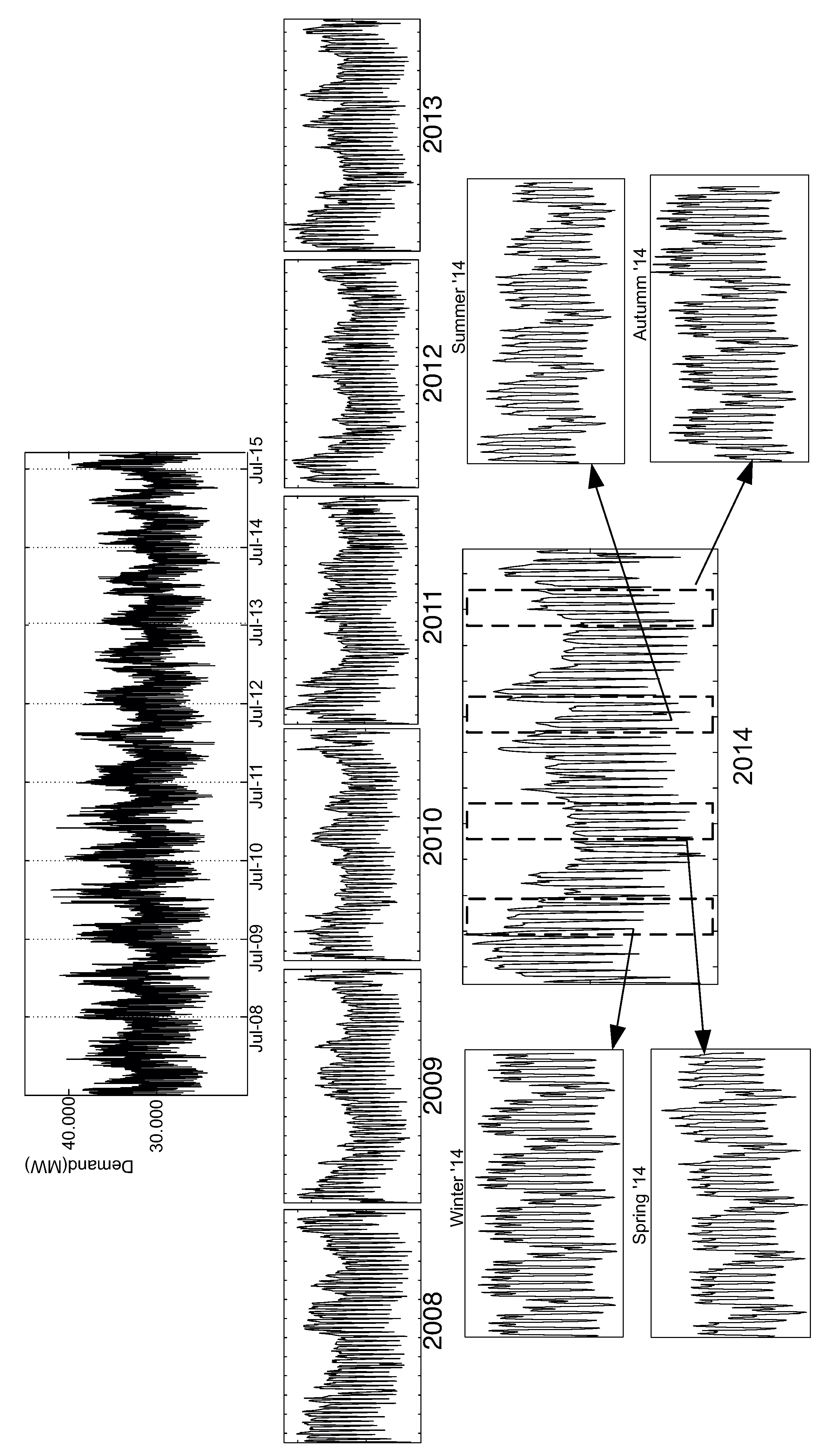
• At least 3 sets of data for each season of the year.
• At least there must be sets in different years, to check the repeatability of the process in similar situations in a matter of period of the year, including holidays nearby.
• The data has not been filtered or the special days were altered.

As a result, for the seasonal double analysis, 250 random samples of 10 weeks were extracted, of which, the first 8 weeks were used for adjustment, while the other two weeks were used for validation. Because the climatic effect present in the series must be assessed, the samples were selected so that they belong to different climatic periods and several years. Figure 1 shows the working scheme for this analysis.

Figure 1. Demand split in years and seasons for stability analysis.

The parameters optimization was done using a minimization algorithm, Nelder-Mead’s simplex [45], where the minimization function was the Root Mean of the Squared Error (RMSE), described in Equation (9).

$$RMSE=\sqrt{\frac{1}{h}\sum _{t=1}^h{({\widehat{X}}_t-X_t)}^2}$$

(9)

where h is the number of samples to be predicted.

Once the model was fit and the parameters obtained, 24-hours ahead forecast during two weeks were performed, and compared against the real data. The forecast accuracy was measured by using the Mean Average Percentage Error (MAPE), described in Equation (10).

$$MAPE(\%)=100\frac{1}{h}\sum _{t=1}^h\frac{\left|{\widehat{X}}_t-X_t\right|}{\left|X_t\right|}$$

(10)

The use of RMSE for the model optimisation is preferred [46]. On the contrary, the most commonly used indicator to compare forecast accuracy is MAPE [47], in special when comparing demand forecasts. The triple seasonal analysis was performed similarly, but it was needed a higher dataset to fit the model and obtain the parameters. Thus, 80 random samples from three full years and two weeks were sampled. The first set of three years was used to fit the model, whereas the two week set was used for validation purposes. In this case, only the $AM{C}_{24,168,8766}$ model was used for the analysis.

4. Results

The analysis procedure was organized inductively. First, the results of the forecasts and how they and the smoothing parameters evolve over time were observed for both double and triple seasonal Holt-Winters models, and then, the influence of the size of the adjusting set was analyzed.

4.1. Double Seasonal Models

Table 2 shows the results of the forecasts made by double seasonal models. In particular, the average of the MAPE when predicting the 250 random samples of two weeks. Only models with the correction of the first order autocorrelation error setting are shown, since they offer better results. Removing the year 2009, the year in which the crisis was emphasized in the Spanish industrial sector until that uncertain moment, the rest of the years there is a clear stability in the forecasts. Holt-Winters models are very robust to small variations. The forecast accuracy values are around 2.6% in terms of MAPE for 24 hours-ahead forecasts. In the triple seasonal case these values are around 7.9% of MAPE.

Table 2. Summary of the 24-hour ahead forecasting MAPE of double seasonal models, split by years.

Year	2008	2009	2010	2011	2012	2013	2014	2015	2016	2017	Mean
$AA{C}_{24,168}$	2.4755	3.3322	2.8705	2.5367	2.6761	2.2657	2.5447	2.4527	2.6741	2.6238	2.6963
$AM{C}_{24,168}$	2.4644	3.2576	2.8389	2.4974	2.5697	2.2284	2.4225	2.4131	2.7129	2.6972	2.6521
$dAA{C}_{24,168}$	2.4402	3.3052	2.8227	2.5120	2.5927	2.2272	2.5114	2.4397	2.6361	2.6189	2.6571
$dAM{C}_{24,168}$	2.4028	3.1723	2.8047	2.4720	2.5209	2.2190	2.3866	2.4164	2.6447	2.5585	2.6034
$DMA{C}_{24,168}$	2.4483	3.3217	2.8034	2.5183	2.6054	2.2351	2.4846	2.4279	2.6399	2.6296	2.6601
$DMM{C}_{24,168}$	2.4119	3.1572	2.8087	2.4519	2.5267	2.2045	2.4077	2.4117	2.6330	2.6184	2.6026
$MA{C}_{24,168}$	2.4722	3.3320	2.8427	2.5260	2.6059	2.2430	2.5031	2.4420	2.6520	2.6325	2.6746
$MM{C}_{24,168}$	2.4462	3.1844	2.8538	2.4670	2.5681	2.2444	2.4787	2.5781	2.7370	2.7615	2.6531
$NA{C}_{24,168}$	2.4434	3.3208	2.8131	2.4970	2.5932	2.2258	2.4869	2.4256	2.6497	2.6216	2.6552
$NM{C}_{24,168}$	2.4061	3.1339	2.8043	2.4196	2.5126	2.1720	2.4407	2.3999	2.6366	2.5810	2.5872

The $NM{C}_{24,168}$ is selected as it offers the best forecast accuracy. As the MAPE provided is an average each year, a split including the months is graphed in Figure 2 as weather conditions and months may influence on the results. Clearly the winter and autumn months have higher levels of MAPE, this time the winter months when worse forecasts occur.

Figure 2. MAPE radar diagram of the forecasts for the $NM{C}_{24,168}$ model using the demand time series from 2008 to 2017.

Table 3 shows the distribution of the parameter values according to the year and seasonal period for the model $NM{C}_{24,168}$. These values were obtained using the sets for adjustment composed of the 250 random samples of 8 weeks. The total row is the mean of the parameters if they are calculated without dividing into seasons. It can be seen that there was a shift in the parameter values from autumn to winter. The values for the daily seasonality are in the order of 0.2 to 0.3 with the exception of winter, where it increases to the value of 0.4. For the intra-weekly seasonality it has a value of 0.2 and it becomes 0.5 for the winter season.

Table 3. Distribution of the parameters for the $NM{C}_{24,168}$ model.

		$\mathit{\alpha }$		${\mathit{\delta }}^{\left(24\right)}$		${\mathit{\delta }}^{\left(168\right)}$		${\mathit{\phi }}_{\mathit{AR}}$
		mean	Dev.	mean	Dev.	mean	Dev.	mean	Dev.
	2009
Autumn		0.0647	0.0398	0.3003	0.0588	0.2660	0.0795	0.8716	0.0487
Spring		0.0099	0.0074	0.3762	0.1326	0.1668	0.0316	0.9480	0.0245
Summer		0.0502	0.0288	0.2407	0.0870	0.2044	0.0637	0.8938	0.0420
Winter		0.6009	0.4141	0.4240	0.2209	0.6386	0.3875	0.6615	0.1899
Total		0.1623	0.2982	0.3331	0.1457	0.3048	0.2548	0.8522	0.1390
	2010
Autumn		0.0805	0.0610	0.2890	0.0281	0.2152	0.0422	0.9011	0.0446
Spring		0.0230	0.0195	0.3029	0.1101	0.2188	0.0505	0.9353	0.0163
Summer		0.0528	0.0075	0.2468	0.0921	0.2518	0.0685	0.8769	0.0279
Winter		0.3968	0.4766	0.3148	0.1564	0.5331	0.4268	0.7537	0.2124
Total		0.1000	0.2056	0.2863	0.0950	0.2696	0.1868	0.8850	0.0966
	2011
Autumn		0.0235	0.0723	0.3017	0.0441	0.2351	0.0839	0.9413	0.0552
Spring		0.0291	0.0238	0.3366	0.1435	0.1973	0.0495	0.9095	0.0448
Summer		0.0804	0.0515	0.2123	0.0563	0.2228	0.0822	0.8846	0.0582
Winter		0.1821	0.3913	0.2925	0.0575	0.4878	0.3039	0.8618	0.1942
Total		0.0624	0.1528	0.2874	0.0971	0.2573	0.1566	0.9063	0.0865
	2012
Autumn		0.0529	0.0456	0.3375	0.0452	0.2340	0.0691	0.9088	0.0480
Spring		0.0244	0.0367	0.3382	0.1281	0.2057	0.0478	0.9430	0.0542
Summer		0.1005	0.0434	0.2259	0.0662	0.2083	0.0373	0.8445	0.0208
Winter		0.4701	0.4720	0.3858	0.2204	0.6269	0.4147	0.6781	0.2440
Total		0.1264	0.2415	0.3179	0.1263	0.2852	0.2258	0.8638	0.1358
	2013
Autumn		0.0429	0.0175	0.3259	0.0798	0.2420	0.0793	0.8560	0.0574
Spring		0.0182	0.0187	0.3160	0.1168	0.1683	0.0606	0.9365	0.0389
Summer		0.0170	0.0187	0.2218	0.0824	0.2306	0.0708	0.9240	0.0541
Winter		0.5574	0.4954	0.5706	0.3562	0.7178	0.3904	0.6341	0.2710
Total		0.1244	0.2932	0.3407	0.2067	0.2992	0.2681	0.8657	0.1650
	2014
Autumn		0.0676	0.0362	0.3823	0.0496	0.2369	0.0866	0.7644	0.1494
Spring		0.0221	0.0205	0.3568	0.1677	0.1965	0.0130	0.9376	0.0361
Summer		0.0139	0.0238	0.1954	0.1014	0.2385	0.0363	0.9537	0.0148
Winter		0.3812	0.4967	0.3156	0.1955	0.4692	0.4601	0.7007	0.1910
Total		0.1212	0.2652	0.3125	0.1414	0.2853	0.2296	0.8391	0.1547
	2015
Autumn		0.0021	0.0021	0.3123	0.0285	0.2428	0.0314	0.9474	0.0133
Spring		0.0440	0.0386	0.3507	0.1349	0.1673	0.0215	0.9199	0.0360
Summer		0.0314	0.0330	0.2616	0.1234	0.2486	0.1469	0.9278	0.0539
Winter		0.3722	0.4874	0.3429	0.2105	0.4552	0.4718	0.6810	0.2140
Total		0.1124	0.2616	0.3169	0.1250	0.2785	0.2390	0.8690	0.1486
	2016
Autumn		0.0443	0.0082	0.3238	0.0165	0.2390	0.0273	0.9209	0.0068
Spring		0.0553	0.0437	0.3345	0.1226	0.2279	0.0868	0.8508	0.1155
Summer		0.0755	0.0304	0.2021	0.0764	0.2380	0.0832	0.8876	0.0036
Winter		0.3290	0.5173	0.2690	0.1228	0.4970	0.4370	0.7450	0.2567
Total		0.1260	0.2536	0.2824	0.0980	0.3005	0.2270	0.8511	0.1385
	2017
Autumn		0.0273	0.0206	0.3193	0.0416	0.2226	0.0298	0.9324	0.0348
Spring		0.0188	0.0182	0.3501	0.1970	0.2208	0.0481	0.9483	0.0277
Summer		0.0494	0.0021	0.3012	0.0305	0.2127	0.0419	0.9225	0.0085
Winter		0.3347	0.5109	0.3765	0.2708	0.4963	0.4366	0.7259	0.2737
Total		0.1075	0.2579	0.3368	0.1476	0.2881	0.2266	0.8823	0.1516

Figure 3 shows a representation of the parameters over time. It can be observed how the values follow a pattern according to the period of the year. The level and AR(1) adjustment values are slightly different from those of the previous analysis. The level values are higher while the AR(1) adjustment is lower. This is because when the trend is removed, possible long-term variations are supplied by the level. The MAPE in winter season worsens while the smoothing parameters increase their variability in autumn. The randomness of the method chosen to analyse variability makes many forecasts done in winter to use a model optimised with data from autumn season. The special events during autumn impact greatly on the winter forecasts.

Figure 3. Radar diagram of the average of the parameters for the model $NM{C}_{24,168}$ depending on the time.

This analysis was completed with a study on the influence of the size of the training dataset on prediction accuracy. The date of 11 July 2016 was set for the 24-hours-ahead forecasts during two weeks, and the size of the training dataset increased from 8 weeks to several years. In this way, it is intended to observe the behaviour of the model with respect to the sample size, following the indications of [41].

Figure 4 presents the MAPE of the 24-hour forecasts according to the size of the sample for the $NM{C}_{24,168}$ and $AM{C}_{24,168}$ models in order to compare their behaviour. It can be observed that the $AM{C}_{24,168}$ model presents higher variability and the model starts to stabilize around the average value 1.7% when a sufficiently large set is used, in particular from 20,000 h. However, the $NM{C}_{24,168}$ model is much more stable, and with relatively small training sets, in particular, with a time series composed of 5000 h, it maintains accuracy values around 1.6%. The $AM{C}_{24,168}$ model is more unstable due to the trend equation (Equation (6)) as the electricity demand time series has no clear trend as shown in Figure 1. Using a larger dataset helps the $NM{C}_{24,168}$ model to stabilize while $AM{C}_{24,168}$ model depends clearly on the season the dataset starts. Although $NM{C}_{24,168}$ model shows better stability than $AM{C}_{24,168}$, the smoothing parameter associated with the trend does not tend to 0 in order to converge to the same model. This is due to the parameters are local optimal, but not global optimal. Thus, the need for an analysis of these parameters and their stability is supported.

Figure 4. MAPE of the 24-hours ahead forecasts according to the size of the datasets used to obtain the model.

Figure 5 shows the evolution of the value of each parameter according to the size of the data set used for the adjustment of the $NM{C}_{24,168}$ model. It can be seen how there is a stabilization of the values in an asymptotic way. It is surprising how the values of the parameters associated with the seasonality exchange the weights as the data set grows. It can be noticed some peaks where the values go up. These peaks coincide with the beginning of the series on holidays. In fact, the most intense peaks coincide with the dates of the Immaculate Conception or Christmas. Once again, a stability in the predictions is observed demonstrating a great predictability. This characteristic does not have the same pattern for all models, and depends largely on the values of the seasonal component, always keeping low values for the $\alpha$ smoothing parameter.

Figure 5. Evolution of parameters versus size of data set.

4.2. Triple Seasonal Models

In this section, an analysis of the parameters of the triple seasonal Holt-Winters models is carried out. Data sets of size 3 years (53 × 24 × 7 × 3 h) were used to adjust the models. As in the case of double seasonal models, 24-hour forecasts were made for two weeks. Although all triple seasonal methods depending on the seasonality and trend were analyzed, there are no major differences between the models, and the $AM{C}_{24,168,8766}$ model turns out to be the easiest to study, as it has 6 parameters, including level, trend, seasonality and fit.

The results obtained are shown in Table 4, where the values of the parameters are organized according to the season and year. In particular, the mean and standard deviation of the smoothing parameters obtained using the 80 sets for adjustment composed of 8 random weeks are shown. It can be noticed that the standard deviation for Autumn of the year 2016 is not defined because it was only a random set of 8 weeks into the Autumn. Contrary to what happens in the double seasonal models, and as seen in the previous section, when using sets of size greater than 20,000 h, the values of the parameters are stabilized.

Table 4. Distribution of smoothing parameters of the $AM{C}_{24,168,8766}$ model.

		$\mathit{\alpha }$		$\mathit{\gamma }$		${\mathit{\delta }}^{\left(24\right)}$		${\mathit{\delta }}^{\left(168\right)}$		${\mathit{\delta }}^{\left(8766\right)}$		${\mathit{\phi }}_{\mathit{AR}}$
		mean	Dev.	mean	Dev	mean	Dev.	mean	Dev.	mean	Dev.	mean	Dev.
	2011
Autumn		0.0008	0.0009	0.0001	0.0000	0.3081	0.0004	0.2296	0.0019	0.0783	0.0306	0.9469	0.0019
Spring		0.0006	0.0008	0.0001	0.0000	0.3137	0.0069	0.2377	0.0183	0.0480	0.0502	0.9463	0.0012
Summer		0.0001	0.0000	0.0001	0.0000	0.3193	0.0094	0.2265	0.0087	0.0718	0.0635	0.9477	0.0014
Winter		0.0001	0.0000	0.0001	0.0000	0.3064	0.0044	0.2144	0.0146	0.1612	0.0038	0.9466	0.0004
Total		0.0003	0.0005	0.0001	0.0000	0.3128	0.0081	0.2267	0.0149	0.0892	0.0604	0.9466	0.0014
	2012
Autumn		0.0001	0.0000	0.0001	0.0000	0.3132	0.0113	0.2446	0.0082	0.0483	0.0682	0.9498	0.0016
Spring		0.0008	0.0009	0.0001	0.0000	0.3032	0.0045	0.2277	0.0018	0.0886	0.0221	0.9438	0.0008
Summer		0.0007	0.0013	0.0001	0.0000	0.3190	0.0090	0.2340	0.0139	0.0684	0.0487	0.9442	0.0017
Winter		0.0004	0.0005	0.0001	0.0000	0.3259	0.0101	0.2404	0.0215	0.0826	0.0386	0.9446	0.0016
Total		0.0005	0.0008	0.0001	0.0000	0.3158	0.0116	0.2344	0.0138	0.0735	0.0405	0.9458	0.0026
	2013
Autumn		0.0001	0.000	0.0001	0.0000	0.3185	0.0079	0.2348	0.0122	0.0802	0.0154	0.9510	0.0003
Spring		0.0001	0.0000	0.0001	0.0000	0.3038	0.0046	0.2280	0.0075	0.0885	0.0328	0.9534	0.0017
Summer		0.0001	0.0000	0.0001	0.0000	0.3147	0.0030	0.2214	0.0060	0.1017	0.0259	0.9515	0.0011
Winter		0.0001	0.0000	0.0001	0.0000	0.3179	0.0133	0.2292	0.0020	0.1481	0.0571	0.9522	0.0014
Total		0.0001	0.0000	0.0001	0.0000	0.3134	0.0090	0.2272	0.0080	0.1064	0.0416	0.9523	0.0014
	2014
Autumn		0.0001	0.0000	0.0001	0.0000	0.3178	0.0100	0.2452	0.0077	0.0467	0.0462	0.9437	0.0005
Spring		0.0001	0.0000	0.0001	0.0000	0.3145	0.0029	0.2251	0.0072	0.0893	0.0126	0.9419	0.0004
Summer		0.0001	0.0000	0.0001	0.0000	0.3235	0.0130	0.2352	0.0094	0.0557	0.0517	0.9429	0.0018
Winter		0.0001	0.0000	0.0001	0.0000	0.3244	0.0032	0.2318	0.0028	0.1003	0.0515	0.9446	0.0022
Total		0.0001	0.0000	0.0001	0.0000	0.3240	0.0084	0.2343	0.0098	0.0731	0.0439	0.9433	0.0016
	2015
Autumn		0.0001	0.0000	0.0001	0.0000	0.2984	0.0095	0.2258	0.0106	0.0983	0.0204	0.9426	0.0014
Spring		0.0001	0.0000	0.0001	0.0000	0.3050	0.0040	0.2279	0.0042	0.0403	0.0147	0.9421	0.0014
Summer		0.0007	0.0010	0.0001	0.0000	0.3134	0.0055	0.2250	0.0127	0.0596	0.0523	0.9411	0.0027
Winter		0.0001	0.0000	0.0001	0.0000	0.3160	0.0068	0.2117	0.0074	0.1377	0.0303	0.9403	0.0003
Total		0.0002	0.0005	0.0001	0.0000	0.3082	0.0092	0.2224	0.0103	0.0840	0.0481	0.9415	0.0017
	2016
Autumn		0.0001	—	0.0001	—	0.3263	—	0.2246	—	0.0399	—	0.9470	—
Spring		0.0001	0.0000	0.00010	0.0000	0.3035	0.0067	0.2262	0.0096	0.0757	0.0273	0.9453	0.0015
Summer		0.0001	0.0000	0.0001	0.0000	0.3112	0.0065	0.2232	0.0055	0.0881	0.0344	0.9457	0.0022
Winter		0.0001	0.0000	0.0001	0.0000	0.3089	0.0040	0.2171	0.0025	0.1301	0.0381	0.9430	0.0008
Total		0.0002	0.0005	0.0001	0.0000	0.3134	0.0097	0.2281	0.0115	0.0862	0.0462	0.9456	0.0038

The value of the ${\delta }^{\left(24\right)}$ parameter stabilizes around 0.3 for any period and with a minimum variability. The value of the ${\delta }^{\left(168\right)}$ parameter stabilizes around 0.2 and the new parameter ${\delta }^{\left(8766\right)}$ around 0.08 and 0.1. These values follow the pattern shown in Figure 5, although there is a transfer between the ${\delta }^{\left(168\right)}$ parameter and the ${\delta }^{\left(8766\right)}$. The introduction of the third seasonality has forced the model to update the intra-weekly seasonality with more recent data over time. On the other hand, values of $\alpha$ stabilize around practically 0, and values of ${\phi }_{AR}$ around 0.95. The existence of so much data makes the AR(1) adjustment practically responsible for adapting the level and makes the level equation redundant. This would imply the elimination of a parameter to be optimized.

In addition, an analysis of the size of the data set and its consequences on the forecasts was carried out in the same way as in the previous case. It was used on the same day, 11 July 2016, where the size of the observed data set was gradually increased and 24-hour forecasts were made over two weeks. The results are shown in Figure 6. An asymptotic evolution towards a MAPE of 2% can be seen. Although the MAPE is triggered and reduced again periodically. The shark fin form responds to an adjusting dataset beginning in the autumn, and finishing in the end of autumn—remember that in autumn the calendar effect was much more important than at other times. One of the main characteristics observed in the triple seasonal models is the variability in predictability, mainly produced by the time of year with more holidays, i.e., autumn.

Figure 6. MAPE of the forecasts for 24-hours ahead according to the size of the dataset used to obtain the $AM{C}_{24,168,8766}$ model.

The selection of 11 July 2016 for the forecasts responds to the necessity to avoid many special events nearby. The nearest one is the 1st May, and the series has enough time to react. As the model has low values for alpha, gamma and ${\delta }_{8766}$, near to zero, only the intraday and intraweek seasonal components can deal and react against the irregularities of the series, smoothing the model to newer values. The closer the start of the autumn period is, the less reaction time the model has to smooth the irregularities. These irregularities affect forecasts more intensely. When forecasting in other dates, the same analysis provides a similar fin-shaped graph. The only difference is the minimum and maximum of the MAPE, that depends on the date chosen.

5. Discussion of the Results

The objective of this section is the empirical analysis of multiple-seasonal Holt-Winters models applied to hourly electricity demand in Spain.

The literature found that analyses the parameters of the models tries to give a solution to the theoretical stability analysis, with the determination of the concept of predictability. However, its application to Holt-Winters models is not direct. It is necessary to carry out an empirical analysis of the models and their forecasts, and from there to draw conclusions about predictability.

A framework was established consisting of the usual process of adjustment and forecasting using a Spanish hourly electricity demand data set provided by REE. The forecasts obtained are then analyzed.

The double seasonal models with an 8 week adjustment period are shown to be robust with respect to predictions. Two different periods, with different characteristics, were used and 24-hour prediction MAPEs of around 2% to 2.6% were obtained. In the models with the best behaviour, the parameters were analyzed, and a direct relationship was found between variability and high values of the smoothing parameters associated with seasonality, and in the periods when a greater number of holidays occur.

The size of the observed data set influences the stability. The MAPE of the $AM{C}_{24,168}$ model has a variability of 0.2%, which from about 20,000 h is reduced to 0.1%. The $NM{C}_{24,168}$ model is much more stable—the series did not show a trend either—achieving this stability in sets longer than 5000 h. As the number of observations increases, the smoothing parameters show a stabilization.

In the case of triple seasonal models, a large number of observations are necessary to adjust the model. Therefore, parameter values are stabilized from the beginning. It can be seen how the predictions get worse when the set of values starts at significant dates in the autumn, a season with many public holidays. Forecasters need to use a dataset avoiding to start in autumn. If no other solution is possible, it is interesting to reduce the dataset size as it is large enough, but not including autumn.

In short, it can be seen that the parameters need a large data set to stabilize, and that the triple seasonal models are not able to improve the double seasonal forecasts due to the calendar effect. As a consequence, it is necessary to develop models that are able to reduce this variability by including the calendar effect in the model.

6. Conclusions

This article analyses the stability of the smoothing parameters in the multiple seasonal Holt-Winters models. This is crucial for the proper appliance of these models to provide accurate and trusted forecasts. Although most of the time, an automatic forecasting algorithm can provide good results, forecasters need to understand the behaviour of these parameters before submitting the forecasts. We use the time series of the hourly Spanish electricity demand.

In this work, we analyze the behaviour of the smoothing parameters of the multiple seasonal Holt-Winters models applied to the series of hourly electricity demand in Spain. There are many variables that affect the parameters within the same time series, including the computation of the initial values, in addition to other factors, such as the calendar or climate conditions. This variability of the parameters is subsequently reflected in the accuracy of the forecasts since they depend greatly on the calculation of the parameters.

The variation of the parameters is analyzed when different seasonal and trend methods are used, as well as different climatic situations of the series. Additionally, it is analyzed how the size of the data set used in order to adjust the model influences on the parameters, and, thus, in the forecasts. It was observed that the seasonal parameters are strongly dependent on the period of the year, making autumn a really difficult period to deal with. This effect is more pronounced in the intra-weekly seasonality than the daily one. However, with the increase in the size of the fitting set, these parameter values stabilise around a value, which depends on the time series. When the size of the set is bigger than 5000 hours, the values are stable. Triple seasonal models have much more stable parameters, although a much larger set of data is necessary to adjust the model. It was found that the main source of variability of the parameters is the calendar effect, which strongly influences the accuracy of the forecasts, not being so much the climatic effect on the series. The accuracy of the forecasts is also stabilised with a larger set of data, it is not necessary to have more than 5000 observations. It is also observed how double seasonal models provide better predictions than triple seasonal ones. The results of the current analysis are limited to being used with Spanish electricity demand. Of course, similar results are expected when faced with load forecasting in other countries or systems. Future works will be addressed toward the development of new models able to include calendar effect in the own model as well as models for the prediction of holidays through the inclusion of discrete seasonalities.

References

- Martínez-Ramos, J.L.; Troncoso, A.; Riquelme-Santos, J.; Gómez-Expósito, A. Short-term hydro-thermal coordination based on interior point nonlinear programming and genetic algorithms. In Proceedings of the IEEE Porto Power Tech Conference, Porto, Portugal, 10–13 September 2001; pp. 1–6. [Google Scholar]
- Hobbs, B.F. Analysis of the value for unit commitment of improved load forecasts. IEEE Trans. Power Syst. 1999, 14, 1342–1348. [Google Scholar] [CrossRef]
- Hong, T. Crystal Ball Lessons in Predictive Analytics. Energybiz 2015, 12, 35–37. [Google Scholar]
- Weron, R. Modeling and Forecasting Electricity Loads and Prices: A Statistical Approach; John Wiley & Sons: Hoboken, NJ, USA, 2013. [Google Scholar]
- Weron, R. Electricity price forecasting: A review of the state-of-the-art with a look into the future. Int. J. Forecast. 2014, 30, 1030–1081. [Google Scholar] [CrossRef]
- Troncoso, A.; Riquelme-Santos, J.M.; Gómez-Expósito, A.; Martínez-Ramos, J.L.; Riquelme, J.C. Electricity Market Price Forecasting Based on Weighted Nearest Neighbors Techniques. IEEE Trans. Power Syst. 2007, 22, 1294–1301. [Google Scholar]
- Chatfield, C.; Mohammad, Y. Holt-Winters Forecasting: Some Practical Issues. J. R. Stat. Soc. Ser. D (The Statistician) 1988, 37, 129–140. [Google Scholar] [CrossRef]
- Gardner, E.S. Exponential smoothing: The state of the art—Part II. Int. J. Forecast. 2006, 22, 637–666. [Google Scholar] [CrossRef]
- Taylor, J.W. Short-term electricity demand forecasting using double seasonal exponential smoothing. J. Oper. Res. Soc. 2003, 54, 799–805. [Google Scholar] [CrossRef]
- Taylor, J.W. Triple seasonal methods for short-term electricity demand forecasting. Eur. J. Oper. Res. 2010, 204, 139–152. [Google Scholar] [CrossRef]
- Taylor, J.W. An evaluation of methods for very short-term load forecasting using minute-by-minute British data. Int. J. Forecast. 2008, 24, 645–658. [Google Scholar] [CrossRef]
- Taylor, J.W.; Espasa, A. Energy forecasting. Int. J. Forecast. 2008, 24, 561–565. [Google Scholar] [CrossRef]
- García-Díaz, J.; Trull, O. Competitive Models for the Spanish Short-Term Electricity Demand Forecasting. In Proceedings of the International Conference on Time Series and Forecasting, Granada, Spain, 27–29 June 2016; pp. 217–231. [Google Scholar]
- Trull, O.; García-Díaz, J.C.; Troncoso, A. Initialization Methods for Multiple Seasonal Holt–Winters Forecasting Models. Mathematics 2020, 8, 268. [Google Scholar] [CrossRef]
- Makridakis, S.; Wheelwright, S.; Hyndman, R. Forecasting: Methods and Applications; John Willey and Sons: Hoboken, NJ, USA, 1998. [Google Scholar]
- Trull, O.; García-Díaz, J.C.; Troncoso, A. Application of Discrete-Interval Moving Seasonalities to Spanish Electricity Demand Forecasting during Easter. Energies 2019, 12, 1083. [Google Scholar] [CrossRef]
- López, M.; Sans, C.; Valero, S.; Senabre, C. Classification of Special Days in Short-Term Load Forecasting: The Spanish Case Study. Energies 2019, 12, 1253. [Google Scholar] [CrossRef]
- Arora, S.; Taylor, J. Short-term forecasting of anomalous load using rule-based triple seasonal methods. IEEE Trans. Power Syst. 2013, 28, 3235–3242. [Google Scholar] [CrossRef]
- David, A.K.; Wen, F. Strategic bidding in competitive electricity markets: a literature survey. In Proceedings of the 2000 Power Engineering Society Summer Meeting (Cat. No. 00CH37134), Seattle, WA, USA, 16–20 July 2000; Volume 4, pp. 2168–2173. [Google Scholar]
- Barroso, L.A.; Cavalcanti, T.H.; Giesbertz, P.; Purchala, K. Classification of electricity market models worldwide. In Proceedings of the International Symposium CIGRE/IEEE PES, San Antonio, TX, USA, 5–7 October 2005; pp. 9–16. [Google Scholar]
- Roldán-Fernández, J.; Gómez-Quiles, C.; Merre, A.; Burgos-Payán, M.; Riquelme-Santos, J.M. Cross-border energy exchange and renewable premiums: The case of the Iberian system. Energies 2018, 11, 3277. [Google Scholar] [CrossRef]
- Domínguez, E.F.; Bernat, J.X. Restructuring and generation of electrical energy in the Iberian Peninsula. Energy Policy 2007, 35, 5117–5129. [Google Scholar] [CrossRef]
- Cancelo, J.R.; Espasa, A.; Grafe, R. Forecasting the electricity load from one day to one week ahead for the Spanish system operator. Int. J. Forecast. 2008, 24, 588–602. [Google Scholar] [CrossRef]
- López, M.; Valero, S.; Senabre, C. Short-term load forecasting of multiregion systems using mixed effects models. In Proceedings of the 2017 14th International Conference on the European Energy Market (EEM), Dresden, Germany, 6–9 June 2017; pp. 1–5. [Google Scholar]
- Talavera-Llames, R.; Pérez-Chacón, R.; Troncoso, A.; Martínez-Álvarez, F. Big data time series forecasting based on nearest neighbours distributed computing with Spark. Knowl. Based Syst. 2018, 161, 12–25. [Google Scholar] [CrossRef]
- Bedi, J.; Toshniwal, D. Deep learning framework to forecast electricity demand. Appl. Energy 2019, 238, 1312–1326. [Google Scholar] [CrossRef]
- Torres, J.F.; Troncoso, A.; Koprinska, I.; Wang, Z.; Martínez-Álvarez, F. Big data solar power forecasting based on deep learning and multiple data sources. Appl. Energy 2019, 238, 1312–1326. [Google Scholar] [CrossRef]
- Yang, Y.; Hong, W.; Li, S. Deep ensemble learning based probabilistic load forecasting in smart grids. Energy 2019, 189, 116324. [Google Scholar] [CrossRef]
- Galicia, A.; Talavera-Llames, R.; Troncoso, A.; Koprinska, I.; Martínez-Álvarez, F. Multi-step forecasting for big data time series based on ensemble learning. Knowl. Based Syst. 2019, 163, 830–841. [Google Scholar] [CrossRef]
- Jiang, W.; Wu, X.; Gong, Y.; Yu, W.; Zhong, X. Holt–Winters smoothing enhanced by fruit fly optimization algorithm to forecast monthly electricity consumption. Energy 2020, 193, 116779. [Google Scholar] [CrossRef]
- Holt, C.C. Forecasting seasonals and trends by exponentially weighted moving averages. Int. J. Forecast. 2004, 20, 5–10. [Google Scholar] [CrossRef]
- Bowerman, B.L.; O’Connell, R.; Koehler, A. Forecasting, Time Series, and Regression: An Applied Approach, 4th ed.; Thomson Brooks/Cole: Belmont, CA, USA, 2005. [Google Scholar]
- Makridakis, S.; Hibon, M. Exponential smoothing: The effect of initial values and loss functions on postsample forecasting accuracy. Int. J. Forecast. 1991, 7, 317–330. [Google Scholar] [CrossRef]
- Archibald, B.C. Parameter space of the Holt–Winters’ model. Int. J. Forecast. 1990, 6, 199–210. [Google Scholar] [CrossRef]
- Lawton, R. How should additive Holt–Winters estimates be corrected? Int. J. Forecast. 1998, 14, 393–403. [Google Scholar] [CrossRef]
- Barnett, S.; Cameron, R.G. Introduction to Mathematical Control Theory, 2nd ed.; Oxford University Press: Oxford, UK, 1985. [Google Scholar]
- Harvey, A.C. Forecasting, Structural Time Series Models and the Kalman Filter; Cambridge University Press: Cambridge, UK, 1990. [Google Scholar]
- Hyndman, R.J.; Akram, M.; Archibald, B.C. Invertibility Conditions for Exponential Smoothing Models; Monash University, Department of Econometrics and Business Statistics: Monash, Australia, 2003. [Google Scholar]
- Hyndman, R.J.; Akram, M.; Archibald, B.C. The admissible parameter space for exponential smoothing models. Ann. Inst. Stat. Math. 2008, 60, 407–426. [Google Scholar] [CrossRef]
- Osman, A.F.; King, M.L. Stability and Forecastability Characteristics of Exponential Smoothing with Regressors Methods. In Proceedings of the Regional Conference on Science, Technology and Social Sciences (RCSTSS 2016), Penang, Malaysia, 4–6 December 2016; pp. 1029–1038. [Google Scholar]
- Hyndman, R.J.; Kostenko, A.V. Minimum sample size requirements for seasonal forecasting models. Foresight 2007, 6, 12–15. [Google Scholar]
- Bermúdez, J. Exponential smoothing with covariates applied to electricity demand forecast. Eur. J. Ind. Eng. 2013, 7, 333–349. [Google Scholar] [CrossRef]
- Troncoso, A.; Riquelme-Santos, J.M.; Riquelme, J.; Gómez-Expósito, A.; Martínez-Ramos, J.L. Time-Series Prediction: Application to the Short-Term Electric Energy Demand. Lecture Notes Comput. Sci. 2004, 3040, 577–586. [Google Scholar]
- Rana, M.; Koprinska, I. Forecasting electricity load with advanced wavelet neural networks. Neurocomputing 2016, 182. [Google Scholar] [CrossRef]
- Nelder, J.A.; Mead, R. A Simplex Method for Function Minimization. Comput. J. 1965, 7, 308–313. [Google Scholar] [CrossRef]
- Hyndman, R.J.; Koehler, A.B. Another look at measures of forecast accuracy. Int. J. Forecast. 2006, 22, 679–688. [Google Scholar] [CrossRef]
- Tofallis, C. A better measure of relative prediction accuracy for model selection and model estimation. J. Oper. Res. Soc. 2015, 66, 1352–1362. [Google Scholar] [CrossRef]