Investigation of Dual-Flow Deep Learning Models LSTM-FCN and GRU-FCN Efficiency against Single-Flow CNN Models for the Host-Based Intrusion and Malware Detection Task on Univariate Times Series Data

Abstract

Intrusion and malware detection tasks on a host level are a critical part of the overall information security infrastructure of a modern enterprise. While classical host-based intrusion detection systems (HIDS) and antivirus (AV) approaches are based on change monitoring of critical files and malware signatures, respectively, some recent research, utilizing relatively vanilla deep learning (DL) methods, has demonstrated promising anomaly-based detection results that already have practical applicability due low false positive rate (FPR). More complex DL methods typically provide better results in natural language processing and image recognition tasks. In this paper, we analyze applicability of more complex dual-flow DL methods, such as long short-term memory fully convolutional network (LSTM-FCN), gated recurrent unit (GRU)-FCN, and several others, for the task specified on the attack-caused Windows OS system calls traces dataset (AWSCTD) and compare it with vanilla single-flow convolutional neural network (CNN) models. The results obtained do not demonstrate any advantages of dual-flow models while processing univariate times series data and introducing unnecessary level of complexity, increasing training, and anomaly detection time, which is crucial in the intrusion containment process. On the other hand, the newly tested AWSCTD-CNN-static (S) single-flow model demonstrated three times better training and testing times, preserving the high detection accuracy.

1. Introduction

In recent years, intrusions into information systems and malware outbreaches as a separate intrusion cases has been one of the leading news topics and results in a significant loss for companies, such as damage of the company’s finances and reputation. According to a 2019 Symantec Internet Security Threat Report, 23% of attack groups are using zero-day vulnerabilities. The Data Breach report of 2019 states that, globally, 60% of companies say they have been breached at some point in their history, with 30% experiencing a breach within the past year alone. In the U.S., the numbers are even higher, with 65% ever experiencing a breach, and 36% within the past year [1]. Influence of ransomware infections in 2018 has grown by 12% for enterprises [2], e.g., LifeLabs Medical Laboratory Services, Canada’s largest lab testing company, paid a ransom after a major cyberattack led to the theft of lab results for 85,000 Ontarians and potentially the personal information of 15 million customers [3]. Industrial control systems (ICSs) are another critical attack vector targeted by the cyber-criminals [4]. In recent years, there have been several important incidents in global ICSs. With the help of operating system vulnerabilities, an Iranian nuclear power station was attacked by Stuxnet in 2010 [5,6] that has caused physical destruction on equipment the computers controlled [7]. Later, in 2014, the ICSs in the energy field of Europe and the United States was attacked by Havex was used to target supervisory control and data acquisition (SCADA) systems [8]. There is no doubt that, to run critical infrastructure or enterprise steadily and reliably, an intrusion detection system (IDS) is one of the most valuable critical tools. It can prevent from data loss, downtime, and damaged equipment, as stated above. It can be seen that, in the majority of modern cyberattacks, some type of malware was used to get access to the system or influence the system state.

That is why intrusion and malware detection tasks have become critical for modern enterprises. The two main technologies utilized for the task are IDS and antivirus (AV). The United States Air Force report published in 1972 by James Anderson gave the first description of an IDS and requirements of such a tool [9]. The main task for them was to alert when unauthorized actions are detected. Automatic systems that cannot only detect but also prevent such actions are called intrusion prevention systems (IPS). IDSs have two primary placement and data collection locations: network and host. Network-based IDS (NIDS) are installed on major data flow points, i.e., switches or routers [10]. However, these systems have no information about the internal state of a host on a network. Host-based IDSs (HIDS) collect data on the end-user machine by monitoring user and host operating system behavior [11]. Since a HIDS is located on the host, it can provide more detailed information about the system state. It also provides context-rich data, allowing better understanding of running processes in the system and decision-making in whether it is or not an intrusion. HIDS are often used in combination with an AV system, which targets one specific malware-based intrusion type. In this paper, we concentrate on host-level intrusion detection, since network-level attack detection is deeply analyzed, and promising results were demonstrated [12,13].

Classical HIDS and AV approaches are based on change monitoring of critical files and malware signatures, respectively, but are not-resistant to zero-day attacks. Some recent research, utilizing relatively vanilla deep learning (DL) methods, has demonstrated good anomaly-based detection results that already have practical applicability due to low false positive rate (FPR) and potential able to detect zero-day attacks [14]. However, more complex DL methods typically provide better results in tasks, such as natural language processing and image recognition tasks, which is why it could be a reasonable task to evaluate the applicability of these methods for anomaly and malware detection on a host level. Experiments were performed using the attack-caused Windows OS system calls traces dataset (AWSCTD) [15], which is currently considered to be the biggest collection of system calls, generated by more than 12,000 of malware samples and exploits, running on Windows OS. Two complex dual-flow models, long short-term memory fully convolutional network (LSTM-FCN) and gated recurrent unit (GRU)-FCN, were tested; these models were previously proved to be the most efficient in tests on many datasets [16,17]. In addition, two newly introduced models, AWSCTD-CNN-LSTM and AWSCTD-CNN-GRU, were tested. The results obtained were compared with simpler single-flow CNN models, both static and dynamic. Although results by the dual-flow models were good (up to 99.2%), the performed analysis showed that they are, in fact, the same as single-flow models (99.3%) if error rate (1%) is evaluated.

Training and anomaly detection times, which are crucial in the intrusion containment process, of dual-flow models, were higher—up to 3- to 7-fold in several cases—compared to single-flow models, making practical use of complex models non-recommendable for the anomaly and malware detection task on system call data presented as univariate times series data. On the other hand, the newly tested AWSCTD-CNN- static (S) single-flow model demonstrated 30% better training and testing times, preserving identically high detection accuracy (99.3%).

2. Prior and Related Work

In order to evaluate new methods for intrusion and malware detection, data collections are required to support the new research findings. Unfortunately, at the moment, old network-based datasets (Defense Advanced Research Projects Agency (DARPA) and Knowledge Discovery in Databases (KDD) Cup 1999) are still used by the majority of researchers: 42% use the KDD Cup dataset, 20% use the DARPA dataset, and 38% other datasets have been used to verify proposed new methods for anomaly detection [18]. The KDD Cup 1999 dataset was collected in 1999 by processing the Transmission Control Protocol (tcp)dump portions of the 1998 DARPA Intrusion Detection System (IDS) Evaluation dataset, created by Lincoln Lab under contract to DARPA [19,20]. Unfortunately, DARPA derived datasets have network data and are perfect for applying in NIDS research [21], leaving host-level attacks apart.

Five main types of data could be named that can be used by the HIDS or AV in order to perform intrusion and/or malware detection:

• System logs and system audit data: These records keep information on operating system generated records that contain information about occurred events: warnings, errors, system failures, etc. [22]. Logs can also be produced by the applications executed on the operating system. Application logs can contain information about user sessions, such as login time, user-program interactions, authentication result, etc. Logs produced by the operating system are typically called system logs, while log records produced by the applications are usually referred to as audit data.
• System calls: System call tracing is a popular source of data for intrusion detection as unusual system call sequences can produce evidence of potential irruptions [23]. System calls as the data source for intrusion and malware detection nowadays are more popular than log files. The main reason for that is that they depict primary data produced by the applications [24] (both legal or malicious), and there is no filtering, interpretation, nor processing applied. Application of system calls for the intrusion detection task is widely discussed [25,26], and its popularity is increasing as new training datasets and machine learning (ML) or DL methods arise [14,15,27,28].
• Windows registry: Windows operating system configuration settings for all programs and hardware on that host are placed in Windows registry. All processes use the registry to achieve their goals. Since malware also falls into that scope [29,30], Windows registry analysis can be seen as a source for analysis by anomaly-based HIDS, while the majority of existing HIDS solutions simply monitor and react to modifications made to the registry [11].
• File system: File system changes are typically made by intruders (changes to configuration files, the introduction of new users, cleaning of log files to hide the intrusion traces, etc.) and malicious applications (code hiding, installation files, etc.). One of the most popular HIDS that monitors changes in critical files is Open Source Host-based Intrusion Detection System (OSSEC) [11,31]. It runs both on Windows and Linux operating systems as agent and reports file changes to the central server. Other notable HIDS systems that work with file system integrity monitoring are Tripwire [32], Disk-Based IDS [33], Storage-Based IDS [34], I3FS [35], and Samhain [36].
• System performance: System performance parameters, such as central processing unit (CPU), random access memory (RAM), network utilization, etc., can also be seen as a valuable source for intrusion and malware detection when exceeding the threshold barrier. For example, Dark-Trace [37] utilizes artificial intelligence (AI) methods for detection of abnormal network flows.

The first HIDS-related data collection was created in 2000 during a KDD dataset assembly and contained event log data of Windows New Technology (NT) host [38]. Nevertheless, KDD Cup-related datasets lack host-related information and are typically used only in NIDS research [39]. Later, in 2015, another database of Windows audit logs was generated by running malware samples, and new malicious behavior detection methods were introduced [40]. In 2016, the Australian Defence Force Academy (ADFA)-IDS dataset, which contains Windows and Linux system calls generated in the experiment when zero-day attacks were simulated, was introduced [39,41,42]. It is rather widely used, but even authors of ADFA-IDS agree that ADFA Windows datasets are incomplete: only basic information was collected, and an insufficient amount of vulnerabilities was used to generate malicious activity [39]. ADFA-IDS was followed by NGIDS-DS (Next-Generation IDS Dataset) in 2017, which consists of a labeled network and host logs that collectively reflect the current Unix infrastructures of different enterprises in both normal and abnormal scenarios [27,43]; unfortunately, it contains only information from Linux machines, while the Windows operating system remains very popular and is considered as the main attack target. In 2018, two datasets containing system calls data on Windows machines were introduced. Scientists at the Canadian Institute of Cybersecurity (CIC) introduced the Communications Security Establishment (CSE)-CIC-IDS2018 dataset, which includes the network traffic and log files of Windows and Linux machines [28]. Still, attention is mainly paid to the network level attacks, such as Brute-force, Heartbleed, Botnet, Denial-of-Service (DoS), Distributed Denial-of-Service (DDoS), Web attacks, and infiltration of the network from inside. To close the gap for the Windows HIDS compatible dataset, we propose the AWSCTD dataset, which contains labeled system calls sequences in the form of univariate times series, generated on a Windows host machine in the presence of a malware and clean applications samples, as well as corresponding network traffic, with modifications made to the registry data and file system [44]. Still, the main AWSCTD dataset strength is a huge collection of system calls that, as it was stated earlier, can be considered as the most reliable source for intrusion and malware detection since they represent low level non-filtered and unprocessed information. AWSCTD, together with ADFA-IDS and NGIDS-DS, can be considered the most comprehensive and is based on modern host-level cyber-attacks.

Traditional machine learning (ML) methods have been widely used for the intrusion detection task. Support Vector Machines (SVM) [45,46,47], Artificial Neural Networks (ANN) [48], k-Means Clustering (kMC) [49], and k-nearest neighbors (KNN) [50,51] are some of the most popular and successful applications. Despite the achieved high results, the performance of traditional methods is decreasing with the increase of data size. Such a scenario is inevitable in a today’s cyber world, where more and more data are required to be collected and analyzed in order to make correct intrusion detection decisions. Such a task, combined with Big Data, requires reanalyzing applicability of traditional ML methods and looking into another promising field, specifically, DL [52,53].

CNNs and recurrent neural networks (RNNs) are the most discussed DL methods. Various configurations and combinations of CNNs and RNNs have been widely used not only in IDS systems but also in other fields [54]. CNNs are based on several convolutions and pooling layers combinations that lead to the last simple ANN layer for the final classification. Use of convolution and pooling layers allows reduction in the size of feature maps [55,56]. Today, CNNs are deployed in many practical applications in the fields of computer vision and natural language processing. CNNs were used by the winners of several competitions, such as ImageNet, Kaggle Facial Expression, Kaggle Multimodal Learning, Kaggle Canadian Institute for Advanced Research (CIFAR)-10, and German Traffic Signs [57,58,59]. RNN has a type of architecture that is typically well suited for learning sequential data, where the next item in the sequence is determined by the previous items. The most widely used RNN configuration is the long short-term memory (LSTM) [60]. Another popular RNN configuration is the gated recurrent unit (GRU) [61]. It is similar to LSTM but has fewer parameters because it lacks an output gate. GRU is mainly applied in natural language analysis and translation.

DL methods for intrusion detection started being using in 2014, when a deep belief network (DBN) was used as a classifier with the combination of restricted Boltzmann machine (RBM) for training and backpropagation for the fine-tuning process of KDD Cup 1999 [62]. Later, when computer processing (especially graphics processing unit (GPU)) capabilities were improved, more complex DL configurations emerged. RNNs were the most apparent methods to adapt for intrusion detection due to the ability to work with time-series data [63,64,65]. CNN networks for malware classification started being used in 2016 [66,67], while the first concept of CNN usage for intrusion detection was proposed in Reference [68] and was later successfully applied by Reference [69,70], with the results up to 99% of network anomaly detection accuracy. Later, DL methods were widely used for the datasets mention above. CNN for HIDS was tested with various sliding window sizes on ADFA-IDS and NGIDS-DS [27]. The results were somehow better than the counterpart of the work in Reference [49], where classical ML methods were applied, with a detection rate (DR) of 60% and False Alarm Rate (FAR; also known as FPR) of 20%. To achieve these results, the input layer of 191 and 151 system calls was used. Other authors have used deep CNNs (dCNNs) to extract useful features from the data and the Softmax classifier to generate the final detection result for the ADFA-IDS dataset. This method enhanced the real-time processing and detection efficiency of intrusion detection systems by 7.3% [71]. In our previous research conducted with the AWSCTD dataset, CNN, LSTM, and GRU methods were evaluated. The maximum achieved accuracy was equal to 94.5% and 99.3% for 100 and 1000 first system calls, respectively, with a simple CNN configuration [14]. In recent years, research on the combination of CNNs and RNNs into one model has shown promising results [72,73,74] and was applied from image recognition to Bitcoin price prediction tasks. This encouraged many researchers to apply similar methods in the IDS research field. The combination of CNN and RNN was applied in NIDS and HIDS: it was tested with the KDD Cup 1999 dataset [75] and Australian Defence Force Academy Linux Dataset (ADFA-LD) [76], and comparable results were achieved.

The motivation for the research described below was to evaluate intrusion detection accuracy and other critical parameters with more complex CNN, LSTM, and GRU configurations applied for the AWSCTD dataset since, as already stated, more complex DL models typically provide better results in certain tasks, such as natural language processing and image recognition.

3. Datasets and Methods

In this paper, we provide results achieved using system call data from the AWSCTD dataset for intrusion and malware detection using a long short-term memory fully convolutional network (LSTM-FCN), which typically achieves state-of-the-art performance in comparison with other FCNs [16] and GRU-FCNs and is said to enhance the classification accuracy in many univariate time series datasets without any additional supporting algorithms requirement [17]. Additionally, two newly-introduced models, AWSCTD-CNN-LSTM and AWSCTD-CNN-GRU, were tested. The results were compared with vanilla single-flow CNN models results. This section presents the dataset used, configuration and parameters of DL models, the results evaluation metrics, and other experimental conditions, such as software and hardware parameters.

3.1. Dataset Used

Our previously introduced dataset, AWSCTD, was used for our experiments [44]. Only one dataset was selected for the tests since the only comparable dataset to AWSCTD is ADFA-IDS, but performing tests on both of them was not practical because of the following reasons:

• Test on ADFA-IDS with simple ML methods performed by other authors [49] demonstrated poorer results compared to the use of AWSCTD [77].
• The data structure of ADFA-IDS is somewhat similar to the AWSCTD, but AWSCTD wins by the amount of data (malware samples and the number of system calls for every malware sample).
• Since the number of system calls in the ADFA-IDS is typically smaller than in AWSCTD, it would be impossible to compare the results for longer system call sequences (>600) that typically produce better intrusion/malware detection results.

The AWSCTD dataset part that contains malware-initiated system calls on Windows OS was used. Malware samples were selected from Virus Share [78] and later appended with the information provided by the Virus Total [79]. System Calls sequences used for our experiment, as well as source code used to train and test ML models, can be found on the GitHub repository [80].

Our earlier experiments with AWSCTD have shown that usable result can be achieved with simple one layer CNN model which consists of the input layer, convolutional layer, global max-pooling layer and output layer [14]. The best results with that configuration were generated for the 1000 first system calls sequences when repetitive calls were reduced, i.e., every sample contains a maximum of two consequent identical application programming interface (API) call instances. The idea of reduction was based on research by Reference [66]. Ninety-nine point three percent accuracy was received with the above-mentioned configuration, which means that the analysis of the first 1000 every program system calls can lead to a successful program-based intrusion or malware detection. Furthermore, up to 90% accuracy was achieved with even less than 40 of the first system calls by the application.

In this paper, we also apply the reduction of system calls to analyze the efficiency (accuracy, FPR, length of system call sequence needed, training time, and other parameters) of more sophisticated DL models. In order to ensure unbiased comparison with vanilla single-flow CNN models, all extracted data samples from the AWSCTD the results will be provided for 10, 20, 40, 60, 80, 100, 200, 400, 600, 800, and 1000 system calls collections (identical to Reference [14]).

3.2. ML Models and Configuration Parameters

In total, seven ML models were used in the intrusion detection experiments. State-of-the-art dual-flow LSTM-FCN (Figure 1) and GRU-FCN (Figure 2) models were selected since typically more complex DL configurations tend to generate better results [81]. Those models consist of two flows that are connected to the last decision-making layer: the CNN and RNN flow (LSTM or GRU, respectively). They have been designed for use in time-series datasets, which often are univariate (contains only one observed parameter). System calls from AWSCTD fit perfectly for such methods.

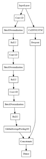
Figure 1. Diagram of long short-term memory fully convolutional network (LSTM-FCN) model. CuDNN = CUDA^® (Compute Unified Device Architecture) Deep Neural Network library (cuDNN); ReLU = rectified linear unit.

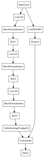
Figure 2. Diagram of gated recurrent unit (GRU)-FCN model.

Apart from that, several additional experimental models, i.e., not described elsewhere previously, were tested. One of the main criteria influencing the model configuration selection was the least possible number of internal nodes in order to ensure reasonable training/testing times while preserving high accuracy and other metrics values. Selection of models was also based on results achieved by Reference [82,83,84], in which DL models (CNN and RNN) were combined in a linear ensemble manner. Combined models returned better accuracy results than separate usage of CNN and RNN models on speech, image, and infrared spectroscopy analysis. The aforementioned research encouraged us to use the linear ensemble with our previously tested [14] models and already recognized as state-of-the-art [85] models:

• Single-flow model (Figure 3), which contains only CNN flow extracted from LSTM-FCN and was originally named FCN in Reference [85].
  

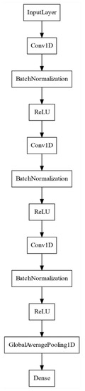  Figure 3. Diagram of FCN model.
• Single-flow CNN model (Figure 4), which demonstrated the best results in our previous experiments [14] and is named AWSCTD-CNN- dynamic (D) (dynamic value of kernels parameter).
  

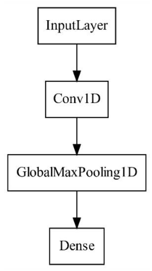  Figure 4. Diagram of AWSCTD-CNN-dynamic (D) and AWSCTD-CNN-static (S) models.
• New single-flow CNN model (Figure 4), named AWSCTD-CNN-S (static value of kernels parameter).
• New dual-flow model (Figure 5), named AWSCTD-CNN-LSTM, combined of AWSCTD-CNN-D and LSTM.
  

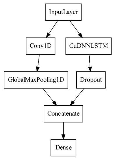  Figure 5. Diagram of attack-caused Windows OS system calls traces (AWSCTD)- convolutional neural network (CNN)-LSTM model.
• New dual-flow model (Figure 6), named AWSCTD-CNN-GRU, combined of AWSCTD-CNN-D and GRU.
  

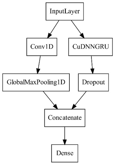  Figure 6. Diagram of AWSCTD-CNN-GRU model.

It can be seen that the LSTM-FCN, GRU-FCN, and FCN consist of a more complex structure in comparison with the AWSCTD-CNN, AWSCTD-CNN-LSTM, and AWSCTD-CNN-GRU models. This feature implies that those models can provide better results in intrusion detection, as suggested in Reference [16,17].

The models were grouped into two families by origin:

1.

FCN family:

• LSTM-FCN
• GRU-FCN
• FCN

2.

AWSCTD family:

• AWSCTD-CNN-D
• AWSCTD-CNN-LSTM
• AWSCTD-CNN-GRU
• AWSCTD-CNN-S

The following specific parameters were used for FCN family models:

3.

The models from FCN family contain original configuration as described in original papers [16,17].

• The FCN-GRU part has 8 unfolds and uses aggressive dropout coefficient of 0.8.
• The CNN part in those models has the following parameters:
• Kernels—128, 256, 128
• Kernel sizes—8, 5, 3
• Kernel initializer—he_uniform
• Activation—tanh.
• Batch normalization parameter of epsilon is 0.01.

The following specific parameters were used for AWSCTD family models:

• The dynamic model AWSCTD-CNN-D is using system calls count as a kernel value: if 1000 system calls sequence is used, then kernel value will be equal to 1000.
• The AWSCTD-CNN-LSTM and AWSCTD-CNN-GRU models also use dynamic unfold value dependant on the number of system calls (one-to-one).
• The dropout value is identical to the FCN family—0.8.
• The static model AWSCTD-CNN-S is using 256 as kernels number for all system calls sequences. The value of 6 is used as the size of kernels since it has been proved as optimal by other authors [86]. Kernel initializer—glorot_uniform. Activation—tanh.

The following configuration parameters were used for all models:

• Epochs—200 (training is stopped if no improvements for six epochs is observed).
• Batch size—20. This value has been selected heuristically to support bigger ML models due to the small amount of RAM available. It is worth mentioning that previous research has used a value of 100. The value of batch is crucial for CNN accuracy results—the higher value is producing better results but is consuming more memory and requires more computational power [87].
• Fold number—5 splits.
• Objective function (or loss function) —binary_crossentropy.
• Optimizer—Adam with default parameters [88].
• Metric to be evaluated by the model during training and testing—accuracy.
• The activation function of the last layer (the layer of decision-making)—sigmoid. The reasoning behind this function—classification is executed in binary mode and for that type of classification sigmoid function produces better results than Softmax.

3.3. Metrics

To evaluate the efficiency of all models the following metrics were defined: accuracy, confusion matrix (CM), precision, recall, F-score, FPR, False Negative Rate (FNR), classification error, and training and testing times. The accuracy metric is calculated for both benign and malware data classes, while the precision, recall, F-score, Matthews Correlation Coefficient (MCC), FPR, FNR, and Error rate are calculated only for the malware class and represent the model capability to perform the intrusion/malware detection task.

The accuracy in this paper is calculated as follows: the method of ML is trained with a portion of the dataset (80%), while another portion (the remaining 20%) of the dataset is used for testing with the trained model, i.e., data used for testing was used for training. Therefore, the percentage of correctly classified records is defined as accuracy [14]. This method is repeated in five K-Folds, and average accuracy based on Keras accuracy metric [89] is used, representing an average classification capability for all classes.

The Confusion Matrix (CM) is where, given a classifier and a set of instances (the test set), a two-by-two CM (also called a contingency table) can be constructed representing the dispositions of the set of instances. This matrix forms the basis for many common metrics [90]. CM used for intrusion classification can be seen in Figure 7.

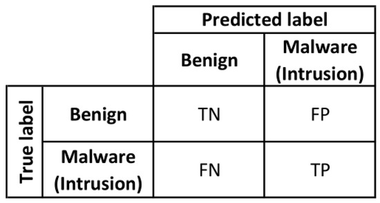
Figure 7. Confusion matrix (CM) of the intrusion classification. TN = true negative; FN = false negative; FP = false positive; TP = true positive.

The precision (also called detection rate) is the fraction of relevant instances among the retrieved instances [90]. It means that, when the model predicts a positive value, what are the odds that the model has made a correct prediction? The precision is calculated as follows:

$$\mathrm{Precision}=\frac{TP}{TP+FP}$$

(1)

The recall, also known as sensitivity, is used to measure the fraction of positive patterns that are correctly classified [90]. In other words, recall is a measure that tells us how great our model is when all the actual values are positive. The recall is calculated as follows:

$$\mathrm{Recall}=\frac{TP}{FN+TP}$$

(2)

The F-score is a metric that combines recall and precision by taking their harmonic mean [90]. F-score is calculated as follows:

$$\mathrm{F} \mathrm{score}=\frac{2\left(Recall Precision\right)}{Recall+Precision}$$

(3)

The MCC is not a biased metric (as precision or recall) and is flexible enough to work properly even with highly unbalanced data. The main properties of MCC are [91]:

• The MCC can be calculated using the CM.
• The calculation of the MCC metric uses the four quantities (TP, TN, FP, and FN), which gives a better summary of the performance of classification algorithms.
• The MCC is not defined if any of the quantities TP + FN, TP + FP, TN + FP, or TN + FN is zero.
• MCC takes values in the interval [−1, 1], with 1 showing a complete agreement, −1 a complete disagreement, and 0 showing that the prediction was uncorrelated with the ground truth.

The MCC value is calculated as follows:

$$\mathrm{MCC}=\frac{TP TN-FP FN}{\sqrt{\left(TP+FP\right)\left(TP+FN\right)\left(TN+FP\right)\left(TN+FN\right)}}$$

(4)

The False Positive Rate (FPR) (also called False Alarm Rate) is calculated as the ratio between the number of negative events wrongly categorized as positive (false positives) and the total number of actual negative events [92]. This parameter in intrusion detection is important because it shows how wrongly a model has classified an action as non-intrusion or valid. The aim is to have as small a FPR as possible to prevent the security personnel from false alarms. FPR is calculated as follows:

$$\mathrm{FPR}=\frac{FP}{FP+TN}$$

(5)

In the same way, the False Negative Rate (FNR) shows the ratio of not detected intrusion attempts and should be also minimized [93]. FNR is calculated as follows:

$$\mathrm{FNR}=\frac{FN}{FN+TP}$$

(6)

The Classification Error (or Error Rate) tells how often the model makes a wrong prediction [90]. The formula for classification error is the following:

$$\mathrm{Classification} \mathrm{error}=\frac{FP+FN}{TP+TN+FP+FN}$$

(7)

The training and testing times demonstrate the time needed to train a model and identify the intrusion/malware, respectively. For intrusion detection, the one-sample test time (decision does it as an intrusion/malware or valid application) is more significant as the ML model is not renewed/trained very often.

3.4. Software and Hardware

The source code was written using the Python language. The special Python libraries were used for the following tasks:

• For DL model creation and configuration—Keras 2.2.4 [89] and Tensorflow 1.12.0 [94] as the backend;
• For data loading, visualization, and pre-processing—Numpy 1.16.5, Pandas 0.24.2, Scikit 0.20.4, and MatPlotLib 2.2.4.

All source code used in this paper is provided on the same repository as AWSCTD [14].

A relatively simple hardware configuration was used to support the above-mentioned software:

• CPU: Intel(R) Core (TM) i5-3570 3.80 GHz (4 Cores, 4 Threads)
• GPU: GTX 1070 (1920 Compute Unified Device Architecture (CUDA^®) Cores)
• RAM: 16GB (DDR3)
• OS: Ubuntu 18.04.3 LTS

The hardware configuration is identical to the experiments presented earlier in Reference [14] for vanilla single-flow models.

4. Results and Discussion

In this section, the experimental results for the metrics (accuracy, CM, precision, recall, F-score, FPR, FNR, classification error, and training and testing times), defined in the previous section, are presented, as well as evaluation of the significance of achieved results by dual-flow models in comparison with vanilla single-flow models. Additionally, the number of epochs needed to reach the saturation and CMs are provided and discussed.

4.1. Accuracy

The accuracy metric demonstrates somewhat similar tendencies for all models—longer system calls sequences tend to provide better results (Table 1).

Table 1. Classification accuracy in percent.

Count	AWSCTD-CNN-S	AWSCTD-CNN-D	AWSCTD-CNN-LSTM	AWSCTD-CNN-GRU	FCN	LSTM-FCN	GRU-FCN
10	88.8	88.0	88.6	89.0	89.3	89.2	88.8
20	91.7	92.7	92.7	92.8	92.3	92.7	92.8
40	92.6	93.8	93.9	93.6	93.6	93.5	93.5
60	94.1	94.2	94.1	93.4	94.0	93.8	93.9
80	94.3	94.3	94.3	94.2	93.8	94.1	94.1
100	94.2	94.4	94.4	94.4	94.4	94.3	94.3
200	94.7	94.5	94.4	94.1	94.8	94.6	94.7
400	95.2	95.0	95.0	95.3	95.0	95.2	95.0
600	98.5	98.6	98.3	98.5	98.3	98.3	98.3
800	98.9	98.9	98.9	98.9	98.6	98.6	98.3
1000	99.3	99.3	99.1	99.2	98.9	98.9	98.8

None of the models reached the 90% accuracy for the sequence of 10 system calls, and the 90% threshold is achieved with 20 system calls sequence by all models. The sequence of 600 system calls can be considered as a threshold that starts providing practically applicable accuracy of more than 98% for all models (Figure 8).

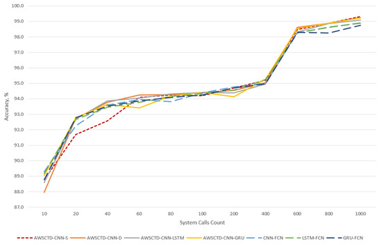
Figure 8. Classification accuracy.

All models are performing almost the same, and there is no clear winner (results vary from 98.8% to 99.3% for the sequence of 1000 system calls). None of the dual-flow FCN family models demonstrates significantly better results than single-flow models, except cases with short system call sequences (up to 10 system calls). Addition of an RNN (LSTM or GRU) layer to the single-flow models also does not result in the expected better accuracy. For longer sequences, single-flow models are demonstrating better accuracy. The reduction of batch size from 100 to 20 had no statistically significant impact on the accuracy of the AWSCTD-CNN-D model.

4.2. Precision, Recall, and F-score

The values of the precision metric demonstrate (Table 2) that all models are detecting malware or intrusion with a probability varying from 0.888 for 10 system calls up to 0.996 for 1000 system calls, i.e., correctness of models can be considered as very high.

Table 2. Precision metric values.

Count	AWSCTD-CNN-S	AWSCTD-CNN-D	AWSCTD-CNN-LSTM	AWSCTD-CNN-GRU	FCN	LSTM-FCN	GRU-FCN
10	0.897	0.906	0.896	0.888	0.891	0.890	0.900
20	0.946	0.932	0.931	0.932	0.939	0.931	0.933
40	0.955	0.941	0.942	0.943	0.937	0.938	0.939
60	0.943	0.946	0.945	0.952	0.944	0.942	0.940
80	0.945	0.945	0.947	0.946	0.944	0.945	0.944
100	0.947	0.948	0.945	0.946	0.947	0.947	0.945
200	0.950	0.950	0.955	0.958	0.952	0.948	0.951
400	0.954	0.959	0.955	0.955	0.952	0.953	0.953
600	0.990	0.990	0.989	0.992	0.992	0.989	0.990
800	0.992	0.993	0.990	0.992	0.994	0.991	0.989
1000	0.995	0.994	0.995	0.996	0.993	0.994	0.992

The recall metric is designed to take evaluate the classification accuracy of intrusions/malware types by classes. In our case, the recall values are higher than corresponding precision values (Table 3). This can be explained by the fact that, in the case of a precision metric, benign system call class has a smaller size and decrease the overall accuracy compared to the recall metric.

Table 3. Recall metric values.

Count	AWSCTD-CNN-S	AWSCTD-CNN-D	AWSCTD-CNN-LSTM	AWSCTD-CNN-GRU	FCN	LSTM-FCN	GRU-FCN
10	0.965	0.941	0.964	0.982	0.980	0.981	0.961
20	0.946	0.977	0.978	0.977	0.962	0.976	0.977
40	0.949	0.982	0.981	0.977	0.983	0.981	0.980
60	0.984	0.982	0.981	0.965	0.981	0.980	0.984
80	0.985	0.984	0.983	0.982	0.979	0.983	0.983
100	0.981	0.983	0.986	0.985	0.983	0.983	0.984
200	0.986	0.983	0.975	0.969	0.984	0.986	0.984
400	0.988	0.981	0.984	0.988	0.988	0.990	0.987
600	0.991	0.992	0.990	0.990	0.987	0.989	0.989
800	0.994	0.993	0.996	0.994	0.990	0.991	0.989
1000	0.997	0.997	0.994	0.995	0.993	0.993	0.993

The F-score metric is calculated from the precision and recall as the harmonic mean of both values. The distribution of this metric is also similar to the accuracy (Table 4)—the longest system calls sequences are producing the best results.

Table 4. F-score metric values.

Count	AWSCTD-CNN-S	AWSCTD-CNN-D	AWSCTD-CNN-LSTM	AWSCTD-CNN-GRU	FCN	LSTM-FCN	GRU-FCN
10	0.930	0.923	0.928	0.932	0.934	0.933	0.929
20	0.946	0.954	0.954	0.954	0.950	0.953	0.954
40	0.952	0.961	0.961	0.960	0.960	0.959	0.959
60	0.963	0.964	0.963	0.958	0.962	0.961	0.962
80	0.964	0.964	0.965	0.964	0.961	0.963	0.963
100	0.964	0.965	0.965	0.965	0.965	0.965	0.964
200	0.967	0.966	0.965	0.963	0.968	0.967	0.967
400	0.971	0.970	0.969	0.971	0.970	0.971	0.969
600	0.991	0.991	0.990	0.991	0.989	0.989	0.989
800	0.993	0.993	0.993	0.993	0.992	0.991	0.989
1000	0.996	0.995	0.994	0.995	0.993	0.993	0.992

The results of precision, recall, and F-score demonstrate that all of the tested models are performing almost the same, and advantage of more complex models cannot be observed. The sequence of 600 system calls remains as the threshold for obtaining noticeably better and practically applicable results.

4.3. MCC

The value of MCC is calculated from all CM parameters. This has an advantage for our imbalanced data. As it can be seen in Table 5, all MCC coefficients are close to 1. That means that models’ predictions are matching with actual results.

Table 5. Matthews Correlation Coefficient (MCC) metric values.

Count	AWSCTD-CNN-S	AWSCTD-CNN-D	AWSCTD-CNN-LSTM	AWSCTD-CNN-GRU	FCN	LSTM-FCN	GRU-FCN
10	0.664	0.648	0.659	0.672	0.680	0.676	0.666
20	0.766	0.788	0.786	0.789	0.777	0.785	0.789
40	0.788	0.816	0.818	0.812	0.810	0.806	0.808
60	0.821	0.826	0.820	0.804	0.817	0.811	0.814
80	0.824	0.825	0.826	0.822	0.811	0.821	0.819
100	0.822	0.828	0.828	0.828	0.828	0.826	0.824
200	0.831	0.826	0.822	0.816	0.833	0.827	0.831
400	0.840	0.836	0.833	0.843	0.834	0.842	0.833
600	0.950	0.954	0.944	0.952	0.943	0.943	0.944
800	0.963	0.963	0.962	0.963	0.955	0.954	0.942
1000	0.977	0.975	0.970	0.974	0.963	0.964	0.959

The 600 system calls sequence repeatedly shows its importance—it improves MCC value by 13% in comparison with 400 system calls sequence (in case of the relatively best performing AWSCTD-CNN-S model).

4.4. FPR and FNR

In the context of intrusion detection, the false/missed alarm (FPR or FNR) is an important metric: a high rate of false alarms disturbs the security staff attention and increases the chance of a missed attack. The minimization of such events is an essential field of IDS research [95]. This metric demonstrates (Table 6) that AWSCTD family models have an advantage against the FCN family: the AWSCTD-CNN-GRU model has the best FPR of 0.018 for 1000 system calls sequence, while LSTM-FCN has the best value of 0.027 for the same sequence, i.e., 50% worse.

Table 6. False positive rate (FPR) metric values.

Count	AWSCTD-CNN-S	AWSCTD-CNN-D	AWSCTD-CNN-LSTM	AWSCTD-CNN-GRU	FCN	LSTM-FCN	GRU-FCN
10	0.368	0.324	0.373	0.414	0.397	0.403	0.357
20	0.179	0.238	0.243	0.237	0.208	0.240	0.236
40	0.156	0.214	0.209	0.205	0.227	0.224	0.220
60	0.213	0.199	0.203	0.176	0.209	0.215	0.225
80	0.211	0.208	0.203	0.206	0.212	0.210	0.213
100	0.200	0.198	0.209	0.205	0.201	0.203	0.211
200	0.205	0.202	0.178	0.167	0.196	0.211	0.199
400	0.198	0.177	0.194	0.194	0.209	0.203	0.204
600	0.041	0.041	0.048	0.035	0.035	0.047	0.044
800	0.033	0.031	0.042	0.035	0.028	0.038	0.046
1000	0.022	0.026	0.022	0.018	0.030	0.027	0.035

The static (AWSCTD-CNN-S) and dynamic (AWSCTD-CNN-D) models demonstrate the lowest FNR values for 1000 system calls—0.003 (Table 7). In comparison, the best achieved FNR result by the FCN family model is equal to 0.007 and is almost 60% worse.

Table 7. False negative rate (FNR) metric values.

Count	AWSCTD-CNN-S	AWSCTD-CNN-D	AWSCTD-CNN-LSTM	AWSCTD-CNN-GRU	FCN	LSTM-FCN	GRU-FCN
10	0.035	0.059	0.036	0.018	0.020	0.019	0.039
20	0.054	0.023	0.022	0.023	0.038	0.024	0.023
40	0.051	0.018	0.019	0.023	0.017	0.019	0.020
60	0.016	0.018	0.019	0.035	0.019	0.020	0.016
80	0.015	0.016	0.017	0.018	0.021	0.017	0.017
100	0.019	0.017	0.014	0.015	0.017	0.017	0.016
200	0.014	0.017	0.025	0.031	0.016	0.014	0.016
400	0.012	0.019	0.016	0.012	0.012	0.010	0.013
600	0.009	0.008	0.010	0.010	0.013	0.011	0.011
800	0.006	0.007	0.004	0.006	0.010	0.009	0.011
1000	0.003	0.003	0.006	0.005	0.007	0.007	0.007

4.5. Error Rate

Error rate values are presented in Table 8. It is consistently seen that the 600 system calls sequence is the first one that generates significantly better results than the smaller ones.

Table 8. Error rate metric values.

Count	AWSCTD-CNN-S	AWSCTD-CNN-D	AWSCTD-CNN-LSTM	AWSCTD-CNN-GRU	FCN	LSTM-FCN	GRU-FCN
10	0.112	0.120	0.114	0.110	0.107	0.108	0.112
20	0.083	0.073	0.073	0.072	0.077	0.073	0.072
40	0.074	0.062	0.061	0.064	0.064	0.065	0.065
60	0.059	0.058	0.059	0.066	0.060	0.062	0.061
80	0.057	0.057	0.057	0.058	0.062	0.059	0.059
100	0.058	0.056	0.056	0.056	0.056	0.057	0.057
200	0.053	0.055	0.056	0.059	0.052	0.054	0.053
400	0.048	0.050	0.050	0.047	0.050	0.048	0.050
600	0.015	0.014	0.017	0.015	0.017	0.017	0.017
800	0.011	0.011	0.011	0.011	0.014	0.014	0.017
1000	0.007	0.007	0.009	0.008	0.011	0.011	0.012

The best results (the smallest number of error rate) equal to 0.007 were obtained by static (AWSCTD-CNN-S) and dynamic (AWSCTD-CNN-D) models. The best value of the FCN family was equal to 0.011 for FCN and LSTM-FCN models. The differences between families are of no significant statistical difference and do not demonstrate the superiority of dual-flow models.

4.6. The Training Time

As it can be seen from Table 9, the static AWSCTD-CNN-S model demonstrates the fastest training time for the 1000 system calls sequence. The next model by speed is FCN, which is slower by around 21%. All other models were slower than AWSCTD-CNN-S, with results varying from 64–618% (Figure 9).

Table 9. Training time for one-fold.

Count	AWSCTD-CNN-S	AWSCTD-CNN-D	AWSCTD-CNN-LSTM	AWSCTD-CNN-GRU	FCN	LSTM-FCN	GRU-FCN
10	30.11	52.09	91.47	81.92	79.56	106.32	102.61
20	44.80	60.18	94.96	97.15	101.43	118.97	122.03
40	43.73	61.18	105.64	115.05	98.51	161.69	137.87
60	51.94	57.38	125.74	129.02	126.90	166.86	148.37
80	63.99	66.29	149.29	144.12	125.75	189.16	162.97
100	82.33	72.16	140.06	128.47	128.59	182.53	187.53
200	100.24	98.69	161.95	197.37	142.61	285.58	248.22
400	147.46	217.77	684.11	256.65	293.85	588.43	465.05
600	279.19	363.71	1190.30	578.03	280.22	1191.68	601.33
800	507.41	852.84	2246.27	887.89	565.09	2059.99	794.29
1000	453.21	745.45	2785.16	1043.92	549.20	3256.41	959.96

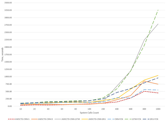
Figure 9. Training time for one-fold.

The training times (Table 9) are given for one-fold. The differentiation in model speeds starts from the sequence of 200 system calls (Figure 9).

The worst training time results were obtained for the LSTM-FCN and AWSCTD-CNN-LSTM models. This can be explained by the number of parameters of these models.

4.7. The Testing Time

The testing time is defined as the time needed to perform classification of one sample. LSTM-based models demonstrate similar behavior, as in the case of training experiments, and require three times more time to perform the detection compared to the best performing AWSCTD-CNN-S model, which retained the leadership, as well as in training task. The testing times for all models and sequence lengths are provided in Table 10.

Table 10. Classification time for one sample.

Count	AWSCTD-CNN-S	AWSCTD-CNN-D	AWSCTD-CNN-LSTM	AWSCTD-CNN-GRU	FCN	LSTM-FCN	GRU-FCN
10	0.00004	0.00004	0.00007	0.00007	0.00011	0.00014	0.00013
20	0.00005	0.00005	0.00009	0.00009	0.00011	0.00015	0.00014
40	0.00007	0.00007	0.00012	0.00013	0.00014	0.00018	0.00018
60	0.00010	0.00009	0.00017	0.00017	0.00016	0.00024	0.00021
80	0.00012	0.00012	0.00021	0.00021	0.00019	0.00027	0.00025
100	0.00016	0.00015	0.00023	0.00025	0.00021	0.00031	0.00029
200	0.00026	0.00030	0.00042	0.00039	0.00034	0.00053	0.00047
400	0.00055	0.00063	0.00123	0.00084	0.00066	0.00128	0.00085
600	0.00138	0.00164	0.00296	0.00172	0.00139	0.00283	0.00173
800	0.00182	0.00218	0.00479	0.00247	0.00194	0.00461	0.00229
1000	0.00223	0.00312	0.00770	0.00347	0.00248	0.00710	0.00283

It can be seen from Figure 10 that static models are more suitable not only for training, but also for classification of long univariate times series data. In our case, it would be long (> 400) system call sequences.

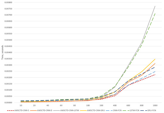
Figure 10. Classification time for one sample.

Since classification time is crucial for attack and malware detection in a real-time application, which could suggest that the best performing AWSCTD-CNN-S is the best suitable candidate for the defined task, despite its relative simplicity.

4.8. The Comparison of the Number of Epochs Needed to Reach the Saturation

The comparison of epochs required to reach the saturation during the training process has demonstrated the correlation to the training time. The relation of accuracy versus epochs for all models presented in Figure 11 for the sequence of 1000 system calls gives the best accuracy.

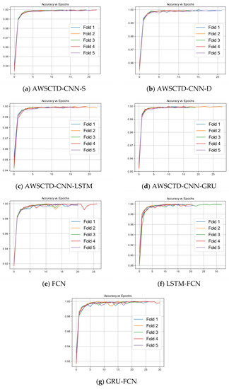
Figure 11. Number of epochs vs. accuracy for the 1000 system call sequence.

The AWSCTD-CNN-S, AWSCTD-CNN-D, and AWSCTD-CNN-LSTM models reached the saturation in maximum of 25 epochs, and they demonstrate better stability. The AWSCTD-CNN-GRU and FCN models required 30 epochs. The maximum number of epochs required by the LSTM-FCN and GRU-FCN models was 30 or more epochs.

4.9. Comparison of the CMs

The values of CMs for 1000 system calls (Figure 12) reveal that the lowest intrusion misclassification values are obtained by static (AWSCTD-CNN-S) and dynamic (AWSCTD-CNN-D) models and are equal to 26 and 25, respectively. The FCN family models generate two times more misclassified results: 53, 55, and 57, respectively, for FCN, LSTM-FCN, and GRU-FCN. The AWSCTD-CNN-GRU model shows the best misclassification value for benign applications, where only 32 items have been identified as an intrusion.

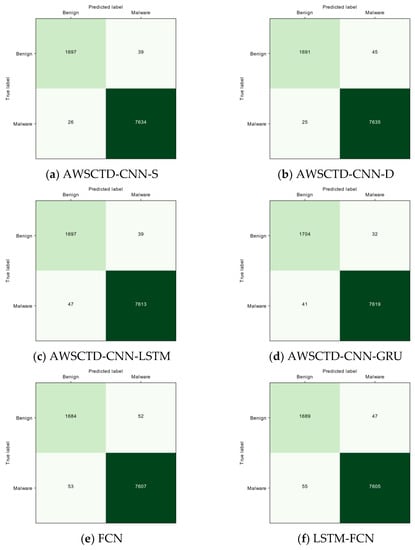
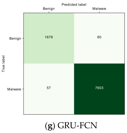
Figure 12. The CM results for 1000 system calls.

Although AWSCTD-CNN-GRU demonstrated the best result for one specific task, AWSCTD-CNN-S can still be considered as the overall winner when taking into consideration all previously discussed metrics.

5. Conclusions

The increasing demand for anomaly-based detection on the host level stimulates the research on ML and DL application for the host-level intrusion and malware detection. Some recent research, utilizing relatively vanilla DL methods, has demonstrated good anomaly-based detection results that already have practical applicability due to low FPR and their ability to potentially detect zero-day attacks. However, it was decided to evaluate the applicability of more complex DL methods that typically provide better results in natural language processing and image recognition tasks.

In total, 7 models were tested: dual-flow LSTM-FCN and GRU-FCN state-of-the-art models that were proved as the most efficient in tests on many datasets; new synthetic dual-flow AWSCTD-CNN-LSTM and AWSCTD-CNN-GRU models, combining CNN and RNN flows; earlier defined single-flow FCN and AWSCTD-CNN-D models; and the newly introduced static single-flow AWSCTD-CNN-S model.

The experiments performed with AWSCTD dataset, containing Windows OS system call sequences by benign and malicious applications in the form of univariate times series data, have not demonstrated any advantages of dual-flow DL models for the host-level intrusion and malware detection task in comparison with the single-flow models. The reached accuracy of dual-flow models was comparable (99.2%) with more vanilla single-flow models (99.3%), taking into account the 1% error rate in case of a sequence of 1000 of system calls. The precision, recall, and F-score results were somewhat identical in their accuracy. On the other hand, dual-flow models were losing the competition in the training and testing time metrics, which are crucial for the intrusion and malware detection tasks. In these metrics, the results for dual-flow models were 3- to 7-fold slower compared to the best performing single flow model, consume more computing resources, and require more epochs to reach the training saturation. The inability of an RNN to boost intrusion detection performance in dual-flow models can be explained by the fact that, in our previous research, single-flow, LSTM, and GRU methods demonstrated worse results, i.e., LSTM (or GRU) flow nodes are reducing CNN achieved accuracy and other metrics.

All tested models were able to reach 90% accuracy with as little as 20 system calls and had practically applicable accuracy of 98% with a sequence of 600 system calls. The relatively best FPR value (approximately 2%) was reached by the AWSCTD-CNN-GRU, while the best FNR value was reached by AWSCTD-CNN-S and AWSCTD-CNN-D models and was equal less 1%. Taking into account all the evaluation metrics, the newly tested AWSCTD-CNN-S can be considered as the overall winner, having the best accuracy (99.3%), shortest training and testing times, and the best FNR rate.

References

- Thales 2019 Thales Data Threat Report—Global Edition. Available online: https://www.thalesesecurity.com/2019/data-threat-report (accessed on 11 December 2019).
- Symantec Internet Security Threat Report 2019. Available online: https://www.symantec.com/content/dam/symantec/docs/reports/istr-24-2019-en.pdf (accessed on 11 December 2019).
- Kiladze, T. LifeLabs Pays Ransom after Massive Data Breach Affecting up to 15 Million Canadians-The Globe and Mail. Available online: https://www.theglobeandmail.com/business/article-lifelabs-pays-ransom-after-massive-data-breach-affecting-up-to-1/ (accessed on 18 December 2019).
- Gonda, O. Understanding the threat to SCADA networks. Netw. Secur. 2014, 2014, 17–18. [Google Scholar] [CrossRef]
- Falliere, N.; Murchu, L.O.; Chien, E. W32.Stuxnet Dossier. Symantec-Secur. Response 2011, 5, 29. [Google Scholar]
- Yang, Y.; McLaughlin, K.; Sezer, S.; Littler, T.; Im, E.G.; Pranggono, B.; Wang, H.F. Multiattribute SCADA-specific intrusion detection system for power networks. IEEE Trans. Power Deliv. 2014, 29, 1092–1102. [Google Scholar] [CrossRef]
- Radziwill, N.M. Countdown to Zero Day: Stuxnet and the Launch of the World’s First Digital Weapon. Qual. Manag. J. 2018, 25, 109–110. [Google Scholar] [CrossRef]
- Walker, D. “Havex” Malware Strikes Industrial Sector Via Watering Hole Attacks. Available online: https://www.scmagazine.com/home/security-news/havex-malware-strikes-industrial-sector-via-watering-hole-attacks/ (accessed on 18 December 2019).
- Anderson, J.P. Computer Security Technology Planning Study. 1972, Volume 2. Available online: https://apps.dtic.mil/docs/citations/AD0758206 (accessed on 18 December 2019).
- Heberlein, L.T.; Dias, G.V.; Levitt, K.N.; Mukherjee, B.; Wood, J.; Wolber, D.D. A Network Security Monitor; Lawrence Livermore National Lab.: Auckland, CA, USA, 1990. [Google Scholar]
- Hay, A.; Cid, D.; Bary, R.; Northcutt, S. OSSEC Host-Based Intrusion Detection Guide; Elsevier: Amsterdam, The Netherlands, 2008; ISBN 9781597492409. [Google Scholar]
- Villalba, L.J.G.; Orozco, A.L.S.; Vidal, J.M. Anomaly-Based Network Intrusion Detection System. IEEE Lat. Am. Trans. 2015, 13, 850–855. [Google Scholar] [CrossRef]
- Le, T.T.H.; Kim, Y.; Kim, H. Network intrusion detection based on novel feature selection model and various recurrent neural networks. Appl. Sci. 2019, 9, 1392. [Google Scholar] [CrossRef]
- Ceponis, D.; Goranin, N. Evaluation of Deep Learning Methods Efficiency for Malicious and Benign System Calls Classification on the AWSCTD. Secur. Commun. Netw. 2019, 2019, 1–12. [Google Scholar] [CrossRef]
- Čeponis, D.; Goranin, N. Towards a Robust Method of Dataset Generation of Malicious Activity for Anomaly-Based HIDS Training and Presentation of AWSCTD Dataset. Balt. J. Mod. Comput. 2018, 6, 217–234. [Google Scholar] [CrossRef]
- Karim, F.; Majumdar, S.; Darabi, H.; Chen, S. LSTM Fully Convolutional Networks for Time Series Classification. IEEE Access 2017, 6, 1662–1669. [Google Scholar] [CrossRef]
- Elsayed, N.; Maida, A.S.; Bayoumi, M. Deep gated recurrent and convolutional network hybrid model for univariate time series classification. Int. J. Adv. Comput. Sci. Appl. 2019, 10, 654–664. [Google Scholar] [CrossRef]
- Azad, C.; Jha, V.K. Data Mining in Intrusion Detection: A Comparative Study of Methods, Types and Data Sets. Int. J. Inf. Technol. Comput. Sci. 2013, 5, 75–90. [Google Scholar] [CrossRef]
- Brugger, T. KDD Cup’99 dataset (Network Intrusion) considered harmful. KDnuggets Newsl. 2007, 7, 15. [Google Scholar]
- Lippmann, R.P.; Fried, D.J.; Graf, I.; Haines, J.W.; Kendall, K.R.; McClung, D.; Weber, D.; Webster, S.E.; Wyschogrod, D.; Cunningham, R.K.; et al. Evaluating Intrusion Detection Systems without Attacking Your Friends: The 1998 DARPA Intrusion Detection Evaluation; Massachusetts Inst of Tech Lexington Lincoln Lab.: Lexington, MA, USA, 1999; Volume 2, pp. 12–26. [Google Scholar]
- Sahu, S.K.; Sarangi, S.; Jena, S.K. A detail analysis on intrusion detection datasets. In Proceedings of the IEEE International Advance Computing Conference (IACC), Gurgaon, India, 21–22 February 2014; pp. 1348–1353. [Google Scholar]
- Rice, R.E.; Borgman, C.L. The use of computer-monitored data in information science and communication research. J. Am. Soc. Inf. Sci. 1983, 34, 247–256. [Google Scholar] [CrossRef]
- Hofmeyr, S.A.; Forrest, S.; Somayaji, A. Intrusion detection using sequences of system calls. J. Comput. Secur. 1998, 6, 151–180. [Google Scholar] [CrossRef]
- Creech, G.; Hu, J. A semantic approach to host-based intrusion detection systems using contiguousand discontiguous system call patterns. IEEE Trans. Comput. 2014, 63, 807–819. [Google Scholar] [CrossRef]
- Forrest, S.; Hofmeyr, S.A.; Somayaji, A.; Longstaff, T.A. A sense of self for Unix processes. In Proceedings of the IEEE Symposium on Security and Privacy, Oakland, CA, USA, 6–8 May 1996; pp. 120–128. [Google Scholar]
- Forrest, S.; Hofmeyr, S.; Somayaji, A. The evolution of system-call monitoring. In Proceedings of the Annual Computer Security Applications Conference (ACSAC), Anaheim, CA, USA, 8–12 December 2008; pp. 418–430. [Google Scholar]
- Tran, N.N.; Sarker, R.; Hu, J. An Approach for Host-Based Intrusion Detection System Design Using Convolutional Neural Network. In Proceedings of the Mobile Networks and Management; Hu, J., Khalil, I., Tari, Z., Wen, S., Eds.; Springer International Publishing: Cham, Switzerland, 2018; pp. 116–126. [Google Scholar]
- Sharafaldin, I.; Lashkari, A.H.; Ghorbani, A.A. Toward generating a new intrusion detection dataset and intrusion traffic characterization. In Proceedings of the International Conference on Information Systems Security and Privacy, Funchal, Portugal, 22–24 January 2018; pp. 108–116. [Google Scholar]
- Hoglund, G.; Butler, J. Rootkits: Subverting the Windows Kernel; Addison-Wesley Professional: Boston, MA, USA, 2005; ISBN 0321294319. [Google Scholar]
- Zavarsky, P.; Lindskog, D. Experimental Analysis of Ransomware on Windows and Android Platforms: Evolution and Characterization. Procedia Comput. Sci. 2016, 94, 465–472. [Google Scholar]
- Lhotsky, B. Instant OSSEC Host-based Intrusion Detection; Packt Publishing Ltd.: Birmingham, UK, 2013; ISBN 9781782167648. [Google Scholar]
- Kim, G.H.; Spafford, E.H. The design and implementation of Tripwire: A file system integrity checker. In Proceedings of the ACM Conference on Computer and Communications Security, Fairfax, VA, USA, 2–4 November 1994. [Google Scholar]
- Griffin, J.; Pennington, A.; Bucy, J. On the Feasibility of Intrusion Detection inside Workstation Disks; Carnegie-Mellon University Pittsburgh Pa School of Computer Science: Pittsburgh, PA, USA, 2003; pp. 1–27. [Google Scholar]
- Pennington, A.G.; Strunk, J.D.; Griffin, J.L.; Soules, C.N.; Goodson, G.R.; Ganger, G.R. Storage-based Intrusion Detection: Watching Storage Activity for Suspicious Behavior. In Proceedings of the USENIX Security Symposium, Washington, DC, USA, 4–8 August 2003; Volume 13, pp. 137–152. [Google Scholar]
- Patil, S.; Kashyap, A.; Sivathanu, G.; Zadok, E. I3FS: An In-Kernel Integrity Checker and Intrusion Detection File System. In Proceedings of the 18th USENIX Large Installation System Administration Conference, Atlanta, GA, USA, 14–19 November 2004. [Google Scholar]
- Tirumala, S.S.; Sathu, H.; Sarrafzadeh, A. Free and open source intrusion detection systems: A study. In Proceedings of the International Conference on Machine Learning and Cybernetics (ICMLC), Guangzhou, China, 12–15 July 2015; Volume 1, pp. 205–210. [Google Scholar]
- Enterprise Immune System. Available online: https://www.darktrace.com/en/technology/#enterprise-immune-system (accessed on 22 February 2020).
- Korba, J. Windows NT Attacks for the Evaluation of Intrusion Detection Systems* Windows NT Attacks for the Evaluation of Intrusion Detection Systems; Massachusetts Inst of Tech Lexington Lincoln Lab.: Lexington, MA, USA, 2000. [Google Scholar]
- Haider, W.; Creech, G.; Xie, Y.; Hu, J. Windows based data sets for evaluation of robustness of Host based Intrusion Detection Systems (IDS) to zero-day and stealth attacks. Futur. Internet 2016, 8, 29. [Google Scholar] [CrossRef]
- Berlin, K.; Slater, D.; Saxe, J. Malicious Behavior Detection using Windows Audit Logs. In Proceedings of the 8th ACM Workshop on Artificial Intelligence and Security; Association for Computing Machinery: New York, NY, USA, 2015; pp. 35–44. [Google Scholar]
- Creech, G.; Hu, J. Generation of a new IDS test dataset: Time to retire the KDD collection. In Proceedings of the IEEE Wireless Communications and Networking Conference (WCNC), Shanghai, China, 7–10 April 2013; pp. 4487–4492. [Google Scholar]
- Creech, G. Developing a High-Accuracy Cross Platform Host-Based Intrusion Detection System Capable of Reliably Detecting Zero-Day Attacks. Ph.D. Thesis, University of New South Wales, Canberra, Australia, 2014; p. 215. [Google Scholar]
- Haider, W.; Hu, J.; Slay, J.; Turnbull, B.P.; Xie, Y. Generating realistic intrusion detection system dataset based on fuzzy qualitative modeling. J. Netw. Comput. Appl. 2017, 87, 185–192. [Google Scholar] [CrossRef]
- Čeponis, D.; Goranin, N. Towards a robust method of dataset generation of malicious activity on a windows-based operating system for anomaly-based HIDS training. In Proceedings of the CEUR Workshop Proceedings, Cotonou, Benin, 3–4 December 2018; Volume 2158. [Google Scholar]
- Horng, S.J.; Su, M.Y.; Chen, Y.H.; Kao, T.W.; Chen, R.J.; Lai, J.L.; Perkasa, C.D. A novel intrusion detection system based on hierarchical clustering and support vector machines. Expert Syst. Appl. 2011, 68, 306–313. [Google Scholar] [CrossRef]
- Khan, L.; Awad, M.; Thuraisingham, B. A new intrusion detection system using support vector machines and hierarchical clustering. VLDB J. 2007, 16, 507–521. [Google Scholar] [CrossRef]
- Kabir, E.; Hu, J.; Wang, H.; Zhuo, G. A novel statistical technique for intrusion detection systems. Futur. Gener. Comput. Syst. 2018, 79, 303–318. [Google Scholar] [CrossRef]
- Ashfaq, R.A.R.; Wang, X.Z.; Huang, J.Z.; Abbas, H.; He, Y.L. Fuzziness based semi-supervised learning approach for intrusion detection system. Inf. Sci. 2017, 378, 484–497. [Google Scholar] [CrossRef]
- Xie, M.; Hu, J.; Yu, X.; Chang, E. Evaluating host-based anomaly detection systems: Application of the frequency-based algorithms to ADFA-LD. In International Conference on Network and System Security; Springer: Cham, Switzerland, 2015. [Google Scholar]
- Aburomman, A.A.; Ibne Reaz, M. Bin A novel SVM-kNN-PSO ensemble method for intrusion detection system. Appl. Soft Comput. J. 2016, 38, 360–372. [Google Scholar] [CrossRef]
- Liao, Y.; Vemuri, V.R. Use of k-nearest neighbor classifier for intrusion detection. Comput. Secur. 2002, 21, 439–448. [Google Scholar] [CrossRef]
- L’Heureux, A.; Grolinger, K.; Elyamany, H.F.; Capretz, M.A.M. Machine Learning with Big Data: Challenges and Approaches. IEEE Access 2017, 5, 7776–7797. [Google Scholar] [CrossRef]
- Kwon, D.; Kim, H.; Kim, J.; Suh, S.C.; Kim, I.; Kim, K.J. A survey of deep learning-based network anomaly detection. Clust. Comput. 2017, 22, 949–961. [Google Scholar] [CrossRef]
- Lipton, Z.C.; Kale, D.C.; Elkan, C.; Wetzel, R. Learning to diagnose with LSTM recurrent neural networks. arXiv 2015, arXiv:1511.03677. [Google Scholar]
- Lecun, Y.; Bottou, L.; Bengio, Y.; Haffner, P. Gradient-based learning applied to document recognition. Proc. IEEE 1998, 86, 2278–2324. [Google Scholar] [CrossRef]
- Dumoulin, V.; Visin, F. A guide to convolution arithmetic for deep learning. arXiv 2016, arXiv:1603.07285. [Google Scholar]
- Russakovsky, O.; Deng, J.; Su, H.; Krause, J.; Satheesh, S.; Ma, S.; Huang, Z.; Karpathy, A.; Khosla, A.; Bernstein, M.; et al. ImageNet Large Scale Visual Recognition Challenge. Int. J. Comput. Vis. 2015, 115, 211–252. [Google Scholar] [CrossRef]
- Graham, B. Fractional Max-Pooling. arXiv 2014, arXiv:1412.6071. [Google Scholar]
- Stallkamp, J.; Schlipsing, M.; Salmen, J.; Igel, C. The German Traffic Sign Recognition Benchmark: A multi-class classification competition. In Proceedings of the International Joint Conference on Neural Networks, San Jose, CA, USA, 31 July–5 August 2011; pp. 1453–1460. [Google Scholar]
- Hochreiter, S.; Schmidhuber, J. Long Short-Term Memory. Neural Comput. 1997, 9, 1735–1780. [Google Scholar] [CrossRef] [PubMed]
- Cho, K.; van Merrienboer, B.; Bahdanau, D.; Bengio, Y. On the Properties of Neural Machine Translation: Encoder-Decoder Approaches. arXiv 2014, arXiv:1409.1259. [Google Scholar]
- Gao, N.; Gao, L.; Gao, Q.; Wang, H. An Intrusion Detection Model Based on Deep Belief Networks. In Proceedings of the 2014 2nd International Conference on Advanced Cloud and Big Data, CBD, Huangshan, China, 20–22 November 2014. [Google Scholar]
- Kim, J.; Kim, H. Applying recurrent neural network to intrusion detection with hessian free optimization. In International Workshop on Information Security Applications; Springer International Publishing: Cham, Switzerland, 2016. [Google Scholar]
- Staudemeyer, R.C. Applying long short-term memory recurrent neural networks to intrusion detection. S. Afr. Comput. J. 2015, 56, 136–154. [Google Scholar] [CrossRef]
- Tang, T.A.; Mhamdi, L.; McLernon, D.; Zaidi, S.A.R.; Ghogho, M. Deep Recurrent Neural Network for Intrusion Detection in SDN-based Networks. In Proceedings of the 4th IEEE Conference on Network Softwarization and Workshops (NetSoft), Montreal, QC, Canada, 25–29 June 2018; pp. 462–469. [Google Scholar]
- Kolosnjaji, B.; Zarras, A.; Webster, G.; Eckert, C. Deep learning for classification of malware system call sequences. In Australasian Joint Conference on Artificial Intelligence; Springer International Publishing: Cham, Switzerland, 2016; pp. 137–149. [Google Scholar]
- Gibert, D. Convolutional Neural Networks for Malware Classification. Ph.D. Thesis, University Rovira I Virgili, Tarragona, Spain, 2016. [Google Scholar]
- Upadhyay, R.; Pantiukhin, D. Application of Convolutional neural networks to intrusion type recognition. In Proceedings of the Presented at the International Conference Engineering & Telecommunications, Moscow, Russia, 18–19 November 2005. [Google Scholar]
- Dawoud, A.; Shahristani, S.; Raun, C. Deep learning for network anomalies detection. In Proceedings of the International Conference on Machine Learning and Data Engineering (iCMLDE), Sydney, Australia, 3–7 December 2018; pp. 117–120. [Google Scholar]
- De Teyou, G.K.; Ziazet, J. Convolutional Neural Network for Intrusion Detection System in Cyber Physical Systems. arXiv 2019, arXiv:1905.03168. [Google Scholar]
- Zhang, S.; Xie, X.; Xu, Y. Intrusion detection method based on a deep convolutional neural network. J. Tsinghua Univ. 2019, 59, 44–52. [Google Scholar]
- Wang, J.; Yang, Y.; Mao, J.; Huang, Z.; Huang, C.; Xu, W. CNN-RNN: A Unified Framework for Multi-label Image Classification. In Proceedings of the IEEE Conference on Computer Vision and Pattern Recognition, Las Vegas, NV, USA, 27–30 June 2016; pp. 2285–2294. [Google Scholar]
- Guo, Y.; Liu, Y.; Bakker, E.M.; Guo, Y.; Lew, M.S. CNN-RNN: A large-scale hierarchical image classification framework. Multimed. Tools Appl. 2018, 77, 10251–10271. [Google Scholar] [CrossRef]
- Ji, S.; Kim, J.; Im, H. A comparative study of bitcoin price prediction using deep learning. Mathematics 2019, 7, 898. [Google Scholar] [CrossRef]
- Vinayakumar, R.; Soman, K.P.; Poornachandrany, P. Applying convolutional neural network for network intrusion detection. In Proceedings of the International Conference on Advances in Computing, Communications and Informatics (ICACCI), Udupi, India, 13–16 September 2017; pp. 1222–1228. [Google Scholar]
- Chawla, A.; Lee, B.; Fallon, S.; Jacob, P. Host based Intrusion Detection System with Combined CNN/RNN Model. In Joint European Conference on Machine Learning and Knowledge Discovery in Databases; Springer International Publishing: Cham, Switzerland, 2018. [Google Scholar]
- Goranin, N.; Čeponis, D. Investigation of AWSCTD dataset applicability for malware type classification. Int. Sci. J. Secur. Futur. 2018, 2, 186–189. [Google Scholar]
- VirusShare.com. Available online: https://virusshare.com/ (accessed on 27 December 2017).
- VirusTotal. Available online: https://www.virustotal.com (accessed on 27 December 2017).
- Čeponis, D.; Goranin, N. AWSCTD: Attack-Caused Windows System Calls Traces Dataset. Available online: https://github.com/DjPasco/AWSCTD (accessed on 24 December 2019).
- Szegedy, C.; Liu, W.; Jia, Y.; Sermanet, P.; Reed, S.; Anguelov, D.; Erhan, D.; Vanhoucke, V.; Rabinovich, A. Going deeper with convolutions. In Proceedings of the IEEE Computer Society Conference on Computer Vision and Pattern Recognition, Boston, MA, USA, 7–12 June 2015. [Google Scholar]
- Deng, L.; Platt, J.C. Ensemble deep learning for speech recognition. In Proceedings of the Fifteenth Annual Conference of the International Speech Communication Association, Singapore, 14–18 September 2014; pp. 1915–1919. [Google Scholar]
- Wen, G.; Hou, Z.; Li, H.; Li, D.; Jiang, L.; Xun, E. Ensemble of Deep Neural Networks with Probability-Based Fusion for Facial Expression Recognition. Cognit. Comput. 2017, 9, 597–610. [Google Scholar] [CrossRef]
- Yuanyuan, C.; Zhibin, W. Quantitative analysis modeling of infrared spectroscopy based on ensemble convolutional neural networks. Chemom. Intell. Lab. Syst. 2018, 181, 1–10. [Google Scholar] [CrossRef]
- Wang, Z.; Yan, W.; Oates, T. Time series classification from scratch with deep neural networks: A strong baseline. In Proceedings of the Proceedings of the International Joint Conference on Neural Networks, Anchorage, AK, USA, 14–19 May 2017. [Google Scholar]
- Tandon, G.; Chan, P.K. Learning Useful System Call Attributes for Anomaly Detection. In Proceedings of the FLAIRS Conference, Clearwater Beach, FL, USA, 15–17 May 2005; pp. 405–411. [Google Scholar]
- Radiuk, P.M. Impact of Training Set Batch Size on the Performance of Convolutional Neural Networks for Diverse Datasets. Inf. Technol. Manag. Sci. 2018, 20, 20–24. [Google Scholar] [CrossRef]
- Kingma, D.P.; Ba, J.L. Adam: A method for stochastic optimization. In Proceedings of the 3rd International Conference on Learning Representations, ICLR 2015-Conference Track Proceedings, San Diego, CA, USA, 7–9 May 2015. [Google Scholar]
- Chollet, F. Keras Documentation. Available online: https://keras.io (accessed on 27 December 2017).
- Fawcett, T. An introduction to ROC analysis. IRBM 2005, 35, 299–309. [Google Scholar] [CrossRef]
- Boughorbel, S.; Jarray, F.; El-Anbari, M. Optimal classifier for imbalanced data using Matthews Correlation Coefficient metric. PLoS ONE 2017, 12, e0177678. [Google Scholar] [CrossRef]
- Axelsson, S. The Base-Rate Fallacy and the Difficulty of Intrusion Detection. ACM Trans. Inf. Syst. Secur. 2000, 3, 186–205. [Google Scholar]
- Joo, D.; Hong, T.; Han, I. The neural network models for IDS based on the asymmetric costs of false negative errors and false positive errors. Expert Syst. Appl. 2003, 25, 69–75. [Google Scholar] [CrossRef]
- Abadi, M.; Barham, P.; Chen, J.; Chen, Z.; Davis, A.; Dean, J.; Devin, M.; Ghemawat, S.; Irving, G.; Isard, M.; et al. Tensorflow: A System for Large-Scale Machine Learning. OSDI 2016, 16, 265–283. [Google Scholar]
- Nguyen, T.H.; Luo, J.; Njogu, H.W. An efficient approach to reduce alerts generated by multiple IDS products. Int. J. Netw. Manag. 2014, 24, 153–180. [Google Scholar] [CrossRef]
© 2020 by the authors. Licensee MDPI, Basel, Switzerland. This article is an open access article distributed under the terms and conditions of the Creative Commons Attribution (CC BY) license (http://creativecommons.org/licenses/by/4.0/).