Highly Curved Lane Detection Algorithms Based on Kalman Filter

Abstract

The purpose of the self-driving car is to minimize the number casualties of traffic accidents. One of the effects of traffic accidents is an improper speed of a car, especially at the road turn. If we can make the anticipation of the road turn, it is possible to avoid traffic accidents. This paper presents a cutting edge curve lane detection algorithm based on the Kalman filter for the self-driving car. It uses parabola equation and circle equation models inside the Kalman filter to estimate parameters of a using curve lane. The proposed algorithm was tested with a self-driving vehicle. Experiment results show that the curve lane detection algorithm has a high success rate. The paper also presents simulation results of the autonomous vehicle with the feature to control steering and speed using the results of the full curve lane detection algorithm.

1. Introduction

The development of the self-driving car is needed for the safety of driver and passenger on the vehicle [1]. Traffic accidents occur for various reasons. The majority of traffic accidents are caused by an improper speed on the road turning or unexpected lane changes when avoiding an obstacle [2]. Some modern cars are already equipped with the emergency braking system, collision warning system, lane-keeping assist system, adaptive cruise control. These systems could be used to help avert traffic accidents when driver is distracted or lost control.

The two most important parts of advanced driver assistance systems are a collision avoidance system and a Lane keeping assist system, which could help to reduce the number of traffic accidents. A fundamental technique for effective collision avoidance and lane-keeping is a robust lane detection method [3]. Especially that method should detect a straight or a curve lane in the far-field of view. A car moving at a given speed will spend a certain time to stop or reduce speed while keeping stability. This means it is necessary to detect road lane in the near field as well as in far-field of view.

Tamal Datta et al. showed a way to detect lane in their lane detection technique [4]. The technique consists of image pre-processing steps (grayscale conversion, canny edge detection, bitwise logical operation) on the image input; it also masked the image according to the region of interest (ROI) in the image. The final stage uses the Hough transformation [5,6] method and detects the lines. Using this method, the parameters for a straight line are achieved. However, their technique did not propose lane detection for curve lanes and can obtain parameters of curve lines (parabola and circle).

A video-based land detection at night was introduced by Xuan He et al. [7]. The method steps include the Gabor filter operator [8] for image pre-processing, adaptive splay ROI, and Hough transform to detect the marker. Lane tracking method that uses Kalman filter [9], is added after lane detection to increase the probability and real-time detection of lane markers. But, their pre-processing steps lack an adaptive auto-threshold method to detect lane in all conditions.

In order to eliminate the uncertainty of lane condition, Shun Yang et al. proposed a replacement of image pre-processing [10]. Their method uses deep learning-based lane detection as a replacement for feature-based lane detection. However, the UNet [11] based encoder-decoder requires high GPU processing unit like Nvidia GPU Geforce GTX 1060 for training and testing. Also, the paper claims CNN-branch is much slower than the feature-based branch in terms of detection rate. The fast detection rate is very important in the case of the autonomous vehicle since the vehicle moves at a very high speed. Also, the result lacks to show results of lane detection in case of the curved lane.

Moreover, Yeongho Son et al. introduced an algorithm [12] to solve the limitation of detecting lane in light illumination change or a shadow or worn-out lanes by using a local adaptive threshold to extract important features from the lane images. Moreover, their paper proposes a feedback RANSAC [13] algorithm to avoid false lane detection by computing two scoring functions based on the lane parameters. They used the quadratic lane model for lane fitting and Kalman filter for smooth lane tracking. However, the algorithm did not provide any close-loop lane keeping control to stay in lane.

Furthermore, a combination of the Hough transform and R-least square method is introduced by Libiao Jiang et al. [14]. They used the Kalman filter to track the lane. Their combination of this method provides results on straight lane marking. Similarly, hazed-based Kalman is used to enhance the information of the road by Chen Chen et al. [15]. Also, Huifend Wang et al. introduced a straight and polynomial curve model to detect the continuity of the lane [16]. The curve fitting method was used to detect the lanes.

In our paper, we introduce a curve lane detection algorithm based on Kalman filter [17]. This algorithm includes Otsu’s threshold method [18,19] to convert RGB to Black-White image, image pre-processing using top view image transform [20,21] to create a top-view image of the road, a Hough transform for detecting the straight lane in the near-field of the sensor [22], and parameter estimation of the curve lane using a Kalman filter. Also, we use two different models for a curve lane in the Kalman filter. One is the parabola model [23], another is the circle model [24]. The Kalman-based linear parabolic lane detection is already tested on consecutive video frames using the parabolic model by K.H. Lim et al. [25]. The paper presents the method which is extended to the circular model. Our proposed method shows robustness against noise. Effective parameter estimation of a curve lane detection could be used to control the speed and heading angle of the self-driving car [26].

Multiple methods have been introduced to detect lane for the self-driving car and advanced driver assistance systems. The vision-based lane detection methods usually used some popular techniques, an edge detector to create a binary image, the classical Hough transform [27,28] to detect straight lines, the color segmentation to extract lane markers, etc.

Most of the methods focused on only a straight lane detection in the near distance using a Hough transform or some simple methods. For a curve lane, few number methods used to detect curved roads such as parabola [23] and hyperbola fitting and B-Splines [29,30], Bezier Splines. To enhance the result of lane detection, the area at the bottom of an image is considered as a region of interest (ROI) [31]. 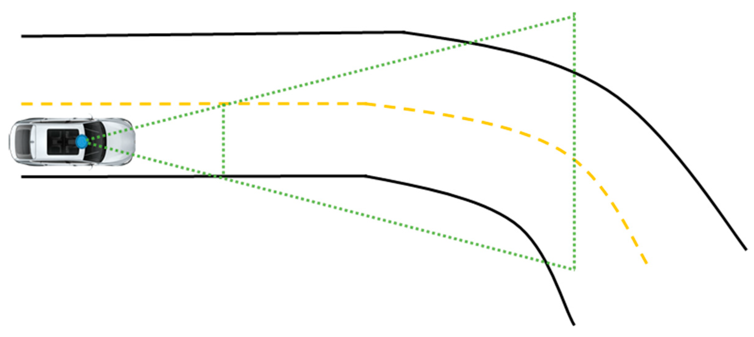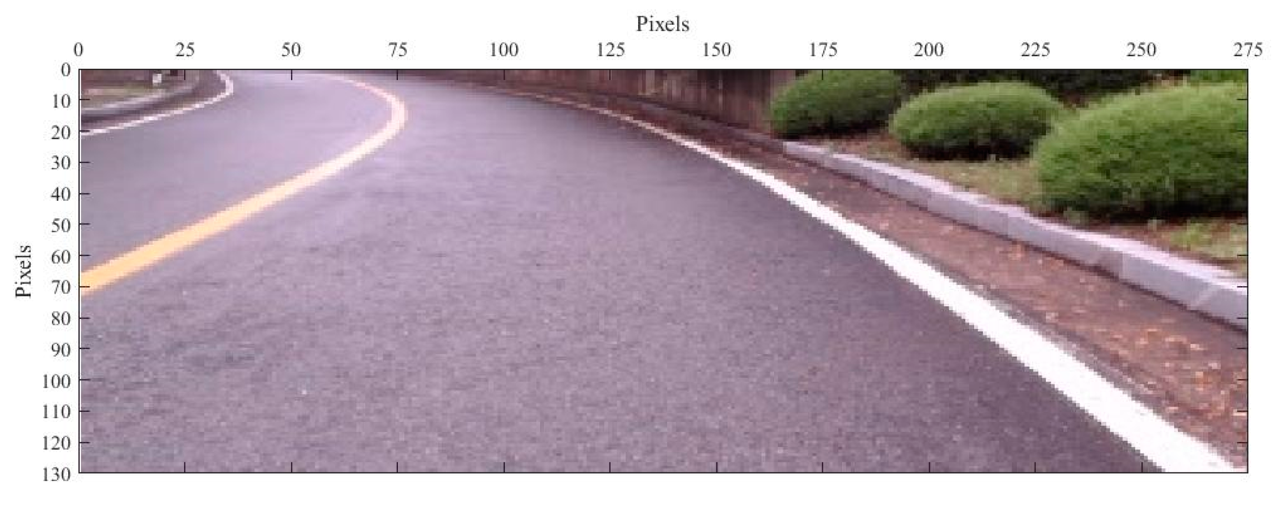Segmenting ROI will increase the efficiency of the lane detection method and eliminate the effect of the upper portion of a road image [32]. The majority of the methods directly detect lanes from the images that are captured by the front-view camera, as shown in Figure 1. However could be robust using the raw image for detect lane, estimating the parameters of road lane may be difficult [33].

This research is considered on a curve lane detection algorithm, which can estimate parameters of the road turning and define geometric shapes based on the mathematical model and the Kalman filter [17].

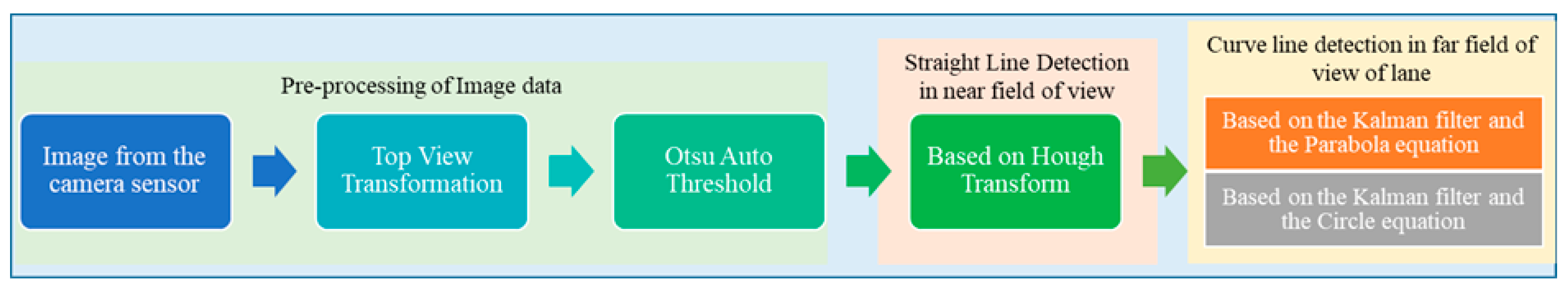
2. Research Method

Our new algorithm consists of two main parts. (1) Image pre-processing. It contains Otsu’s threshold method [19] and top view image transform [20] to create a top-view image of the road. Hough transform predict the straight lane in the near-field of view. (2) A curve lane detection. We use the Kalman filter to detect a curve lane in the far-field of view. This Kalman filter algorithm includes two different methods, the first method is based on the parabola model [23], and the second method is based on the circle model [24]. This method shown in Figure 2 can estimate parameters of the road turning and find geometric shapes based on the mathematical model and the Kalman filter.

2.1. Otsu Threshold

In 1978 inventor Nobuyuki Otsu introduced a new threshold technique. The Otsu threshold technique uses statistical analysis, which can be used to determine the optimal threshold for an image. Nobuyuki Otsu introduced a problem with one threshold for two classes and later extended to a problem with multiple thresholds. For the two classes, this technique assumes the image containing two classes of pixels following bi-modal histogram, foreground pixels, and background pixels. The Otsu threshold method minimizes the sum of the weighted class variances. He named this sum within-class variance and defines it as Equation (1):

$${\sigma }_w^2={\omega }_1{\sigma }_1^2+{\omega }_2{\sigma }_2^2,$$

(1)

The criterion tries to separate the pixels, such that the classes are homogeneous in themselves. Since a measure of group homogeneity is the variance, the Otsu criterion follows consequently. Therefore, the optimal threshold is the one, for which the within-class variance is minimal. In order to find the optimal threshold instead of minimizing the within-class variance is defined as Equation (2):

$$\{\begin{array}{l}{\sigma }_B^2={\omega }_1{\left({\mu }_1-{\mu }_T\right)}^2+{\omega }_2{\left({\mu }_2-{\mu }_T\right)}^2\\ {\mu }_T={{\displaystyle \sum }}_{i=1}^{L}p\left(i\right)·i\end{array}$$

(2)

where ${\mathsf{\mu }}_T$ is the total mean calculated over all gray levels. So the task of finding the optimal set of thresholds $\left[t_1^{\ast },t_2^{\ast },\dots t_{M-1}^{\ast }\right]$ in Equation (3) is either to find the thresholds, which minimize the within-class variance or to find the ones, which maximize the between-class variance. The result is the same.

$$\left[t_1^{\ast },t_2^{\ast },\dots t_{M-1}^{\ast }\right]=argmin\left\{{\sigma }_w^2\right\}=argmax\left\{{\sigma }_B^2\right\},$$

(3)

2.2. Top View Image Transformation

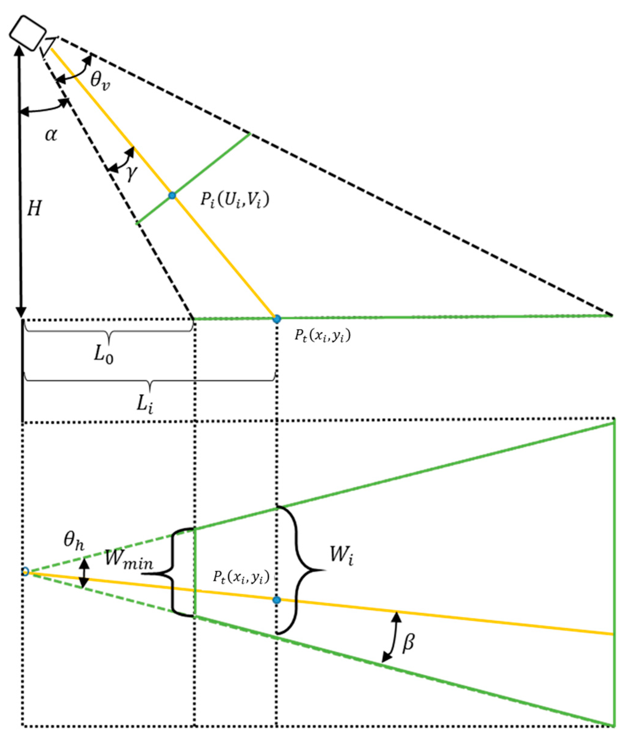
The second step in our algorithm is to create a top view image of the road. The output image is the top view or bird’s view of the road where lanes will be parallel or close to parallel after this transformation. Also, this transformation converts from pixels in the image plane to the world coordinate metric. If necessary we can measure distance using that transformed image.

Figure 3 illustrates the geometry of the top-view image transformation. For the transformation, we need some parameters, where ${\theta }_h$ is the horizontal view angle of the camera, ${\theta }_v$ is the vertical view angle of the camera, $H$ is the height of the camera located, and $\mathsf{\alpha }$ is the tilt angle of the camera.

The height of the camera located in the vehicle is measured in the metric system. We can create two types of top-view image, one is measured by metric using H parameter, another is measured by pixel using $H_{pixel}$ parameter. V is the width of the front view image $P_i\left(U_i,V_i\right)$ and is proportional to W_min of the top view image field illustrated in Figure 3. Equations (4) and (5) show the relationship between the H measured by metric and $H_{pixel}$ measured by pixel.

$$\{\begin{array}{l}{L}_{min}=H\ast \tan \left(\alpha \right)\\ W_{min}=2\ast L_{min}\ast \tan \left({\theta }_h/2\right)\\ K=V/W_{min}\end{array},$$

(4)

Coefficient K is used to transform the metric into the pixel data.

$$\{\begin{array}{l}{H}_{pixel}=H·K\\ \gamma ={\theta }_v·\left(\frac{U-U_i}{U}\right)\\ x_i=L_i-L_0=H_{pixel}\ast \tan \left(\alpha +\gamma \right)-H_{pixel}\ast \tan \left(\alpha \right)\end{array}$$

(5)

According to the geometrical description shown in Figure 3, for each point $P_i\left(U_i,V_i\right)$ on the front view image, the corresponding sampling point $P_t\left(U_i,V_i\right)$ on the top view image can be calculated by using the previous Equations (4)–(6).

$$\{\begin{array}{l}\beta ={\theta }_h·\left(\frac{V-V_i}{V}\right)\\ y_i=L_i·\tan \left({\theta }_h-\beta \right)\end{array}$$

(6)

Then RGB color data are copied from the $\left(U_i,V_i\right)$ position of the front view camera image to the $\left(x_i,y_i\right)$ position of the top view image.

After top-view image transformation, line detection becomes a simple process, which only detects parallel lines that are generally separated by a given, fixed distance. The next step is to detect a straight lane using the Hough transform.

2.3. Straight Lane Detection with Hough Transform

In the near view image, a straight line detection algorithm is formulated by using a standard Hough transformation. The Hough transform also detects many incorrect lines. We need to eliminate the incorrect lanes to reduce computational time and complexity [34].

To remove incorrect lines using the same algorithms on the road lane, the removal of detected lines is needed in which the vehicle is not in. For example, after Hough transformation on the binary image, the longest two lines will be chosen to avoid the issue. The detection for curve lane will start at the finishing points of those two longest two lines which were chosen based on length.

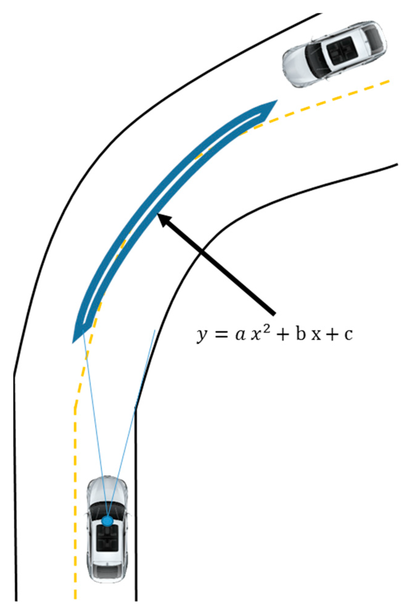
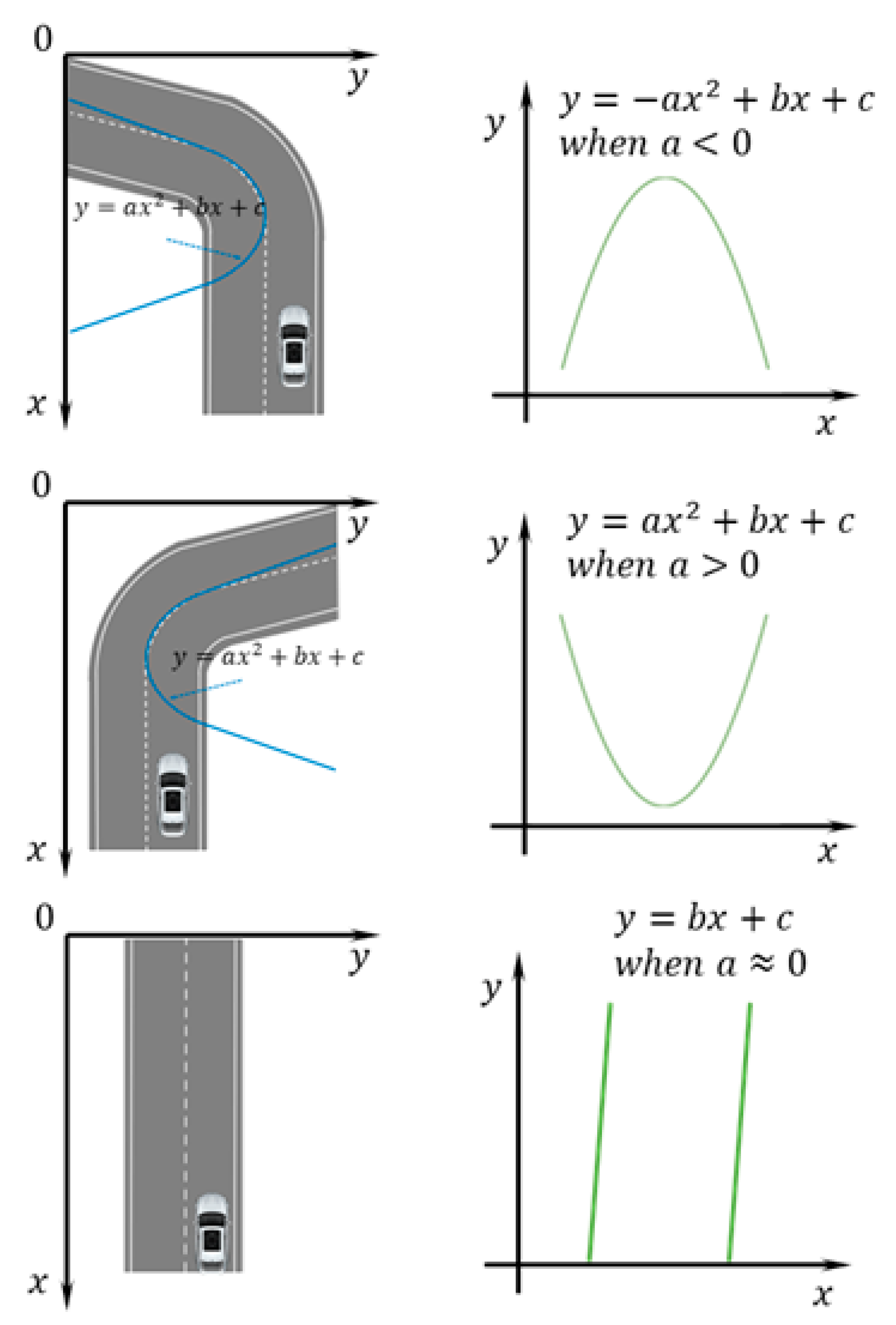
2.4. Curve Lane Detection Based on Kalman Filter and Parabola Equation

In this paper, the most important part is the curve line detection part. This method should detect a straight or a curve line in the far-field of view. Image data (white points in the far-field of view) include uncertainties and noise generated during capturing and processing steps. Therefore, as a robust estimator against these irregularities, a Kalman filter was adopted to form an observer [22]. First of all, we need to define the equation of the curve line, which is a non-linear equation. For the curve line, the best-fit equations are the parabola equation and the circle equation.

In this part, we consider a curve lane detection algorithm which is based on the Kalman filter and Parabola equation. From parabola equation $y=a{x}^2+bx+c$ we need to define three parameters using at least three measurement data. Equations (7) and (8) show system equation of the parabola. Figure 4 illustrates the basic parabolic model of road turning.

$$\{\begin{array}{l}{y}_{i-1}=a{x}_{i-1}^2+b{x}_{i-1}^1+c{x}_{i-1}^0\\ y_i=a{x}_i^2+b{x}_i^1+c{x}_i^0\\ y_{i+1}=a{x}_{i+1}^2+b{x}_{i+1}^1+c{x}_{i+1}^0\end{array}$$

(7)

$$\left[\begin{array}{ccc}{x}_{i-1}^2& x_{i-1}^1& x_{i-1}^0\\ x_i^2& x_i^1& x_i^0\\ x_{i+1}^2& x_{i+1}^1& x_{i+1}^0\end{array}\right]\left[\begin{array}{c}a\\ b\\ c\end{array}\right]=\left[\begin{array}{c}{y}_{i-1}\\ y_i\\ y_{i+1}\end{array}\right]$$

(8)

where $x_{i-1},x_i,x_{i+1}$ and $y_{i-1},y_i,y_{i+1}$ are the measurement data of the curve line detection process. In our case, the measurement data are the coordinates of the white points in the far section.

From Equation (9) we can estimate $a,b,c$ parameters easily.

$$\left[\begin{array}{c}a\\ b\\ c\end{array}\right]=\left(inv\left[\begin{array}{ccc}{x}_{i-1}^2& x_{i-1}^1& x_{i-1}^0\\ x_i^2& x_i^1& x_i^0\\ x_{i+1}^2& x_{i+1}^1& x_{i+1}^0\end{array}\right]\right)\left[\begin{array}{c}{y}_{i-1}\\ y_i\\ y_{i+1}\end{array}\right]$$

(9)

Using this matrix form we can implement our Kalman filter design for curve lane detection. Two important matrices of the Kalman filter are the measurement transition matrix (H) and the state transition matrix (A). It can be expressed as Equation (10):

$$\left[Y_i\right]=\left[H_i\right]\left[X_i\right]$$

(10)

In our case, the measurement transformation matrix $\left[H_i\right]$ contains three white points coordinate values of $x$ axis rearranging the calculation as Equation (11). But, the transition matrix is the identity matrix, because of our Kalman filter design used for the image process.

$$\left[Y_i\right]=\left[\begin{array}{c}{y}_{i-1}\\ y_i\\ y_{i+1}\end{array}\right] \left[H_i\right]=\left[\begin{array}{ccc}{x}_{i-1}^2& x_{i-1}^1& x_{i-1}^0\\ x_i^2& x_i^1& x_i^0\\ x_{i+1}^2& x_{i+1}^1& x_{i+1}^0\end{array}\right] \left[X_{prior}\right]=\left[\begin{array}{c}a\\ b\\ c\end{array}\right]$$

(11)

These two matrices are often referred to as the process and the measurement models, as they serve as the basis for a Kalman filter. The Kalman filter has two steps: the prediction step and the correction step. The prediction step can be expressed as follows, Equations (12) and (13):

$$X_{post}=A_i{X}_{prior}+B{u}_k;\left[X_{post}\right]=\left[X_{prior}\right]$$

(12)

$$P_{post}=A_i{P}_{prior}{A}_i^T+Q_r; P_{post}=P_{prior}+Q_r$$

(13)

where $P_{post}$ is the covariance of the predicted state. The correction steps of the Kalman filter can be expressed through the following Equations (14), (15) and (17).

$$K_{i+1}=(P_{post}{H}^T){\left(H{P}_{post}{H}^T+\mathrm{R}\right)}^{-1}+Q_r$$

(14)

$$X_{post}=X_{prior}+K\left(z_i-H_i{X}_{prior}\right); z_i=\left[\begin{array}{c}{y}_{meas\left(i-1\right)}\\ y_{meas\left(i\right)}\\ y_{meas\left(i+1\right)}\end{array}\right]$$

(15)

where $K_{i+1}$ is the Kalman gain, $X_{post}$ is the a posteriori estimate state at the $i$-th white point. $P_{post}$ is the a posteriori estimate error covariance matrix at the $i$-th white point in the Equation (17).

The Equation (16) shows a matrix form of a posteriori estimate state.

$$\left[\begin{array}{c}{a}_{i+1}\\ b_{i+1}\\ c_{i+1}\end{array}\right]=\left[\begin{array}{c}{a}_i\\ b_i\\ c_i\end{array}\right]+K\left(\left[\begin{array}{c}{y}_{meas\left(i-1\right)}\\ y_{meas\left(i\right)}\\ y_{meas\left(i+1\right)}\end{array}\right]-\left[\begin{array}{ccc}{x}_{i-1}^2& x_{i-1}^1& x_{i-1}^0\\ x_i^2& x_i^1& x_i^0\\ x_{i+1}^2& x_{i+1}^1& x_{i+1}^0\end{array}\right]\left[\begin{array}{c}{a}_i\\ b_i\\ c_i\end{array}\right]\right)$$

(16)

$$P_{post}=\left(I-K{H}_i\right)P_{prior}$$

(17)

To evaluate the viability of the proposed algorithms, we tested the parabola equation using both real data and noisy measurement data in Matlab. The Kalman filter can estimate the parameters of the parabola equation from noisy data. The result section shows a comparison between the measurement value and estimation value, the real value. Figure 5 shows the expected results of left and right turning on the road using the parabolic model based on the Kalman filter [35].

From all these experiment results from the result section, we can see one relationship between road turning and “a” parameter of our approach. If the road is turning toward the left side, the “a” parameter is lower than zero. If the road is turning toward right side, “a” parameter is higher than zero and if the road is straight, “a” parameter is almost equal to zero. This process is shown in Figure 6.

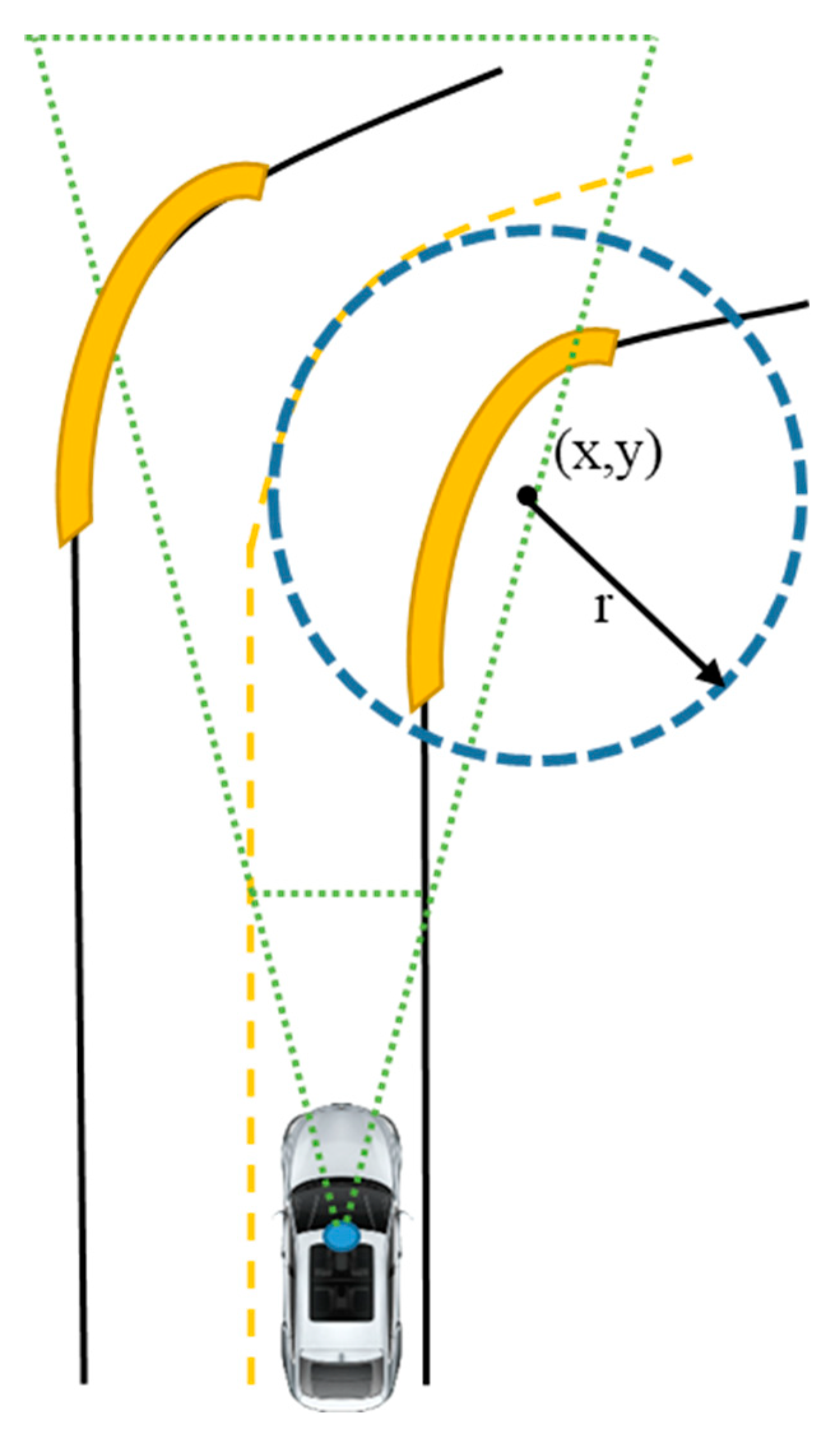
2.5. Curve Lane Detection Based on Kalman Filter and Circle Equation

For the curve line, the second-best fit equation is the circle equation, shown in Figure 7. In this part, we consider curve line detection algorithms [24] based on the Kalman filter and circle equation. From the circle equation $r^2={\left(x-h\right)}^2+{\left(y-k\right)}^2$ we need to define circle radius $r$ and the center of circle $\left(h,k\right)$.

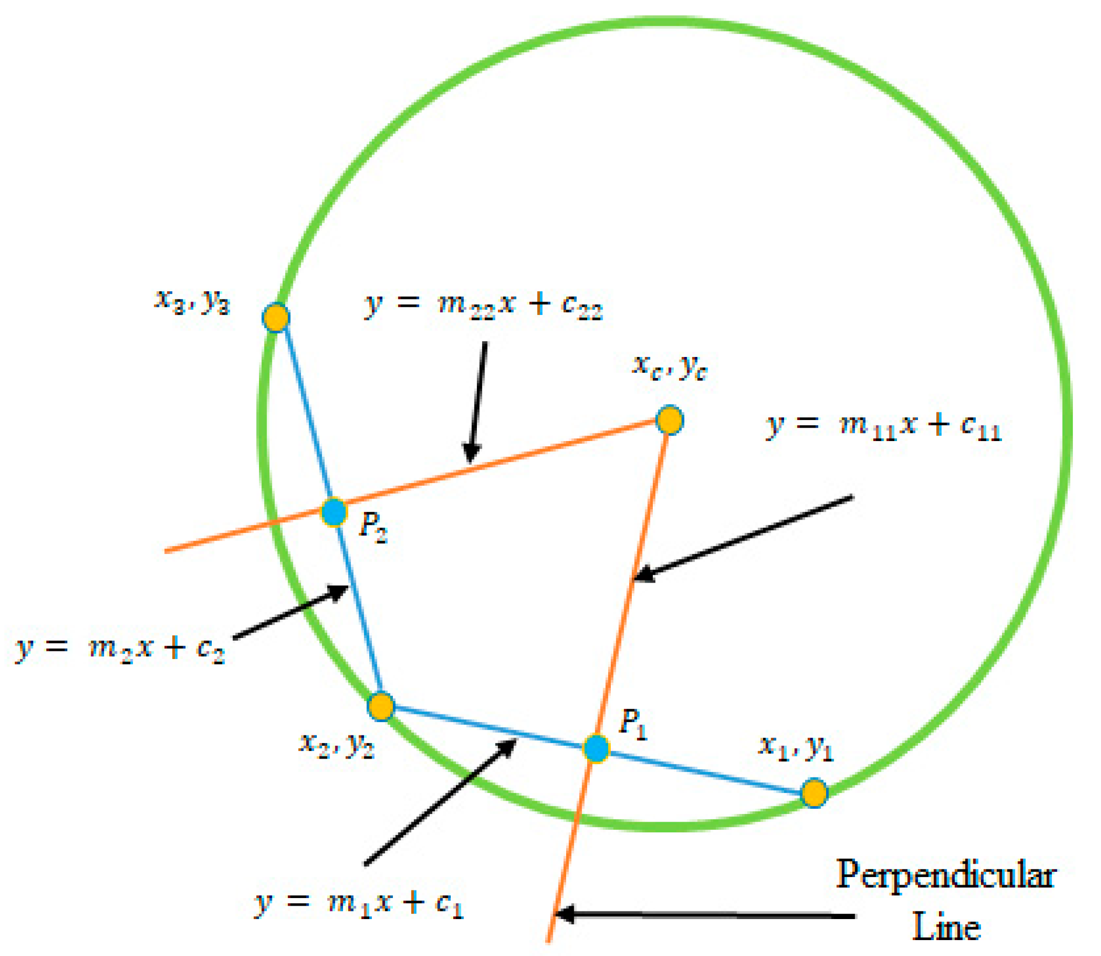
Using every three points of a circle we can draw a pair of chords. Based on these two chords we can calculate the center of the circle [36]. If we have $n$ number points, it is possible to calculate $n-2$ number center.

Pairs of chords in each chain are used to calculate the center. Here, $\left(x_1,y_1\right)$, $\left(x_2,y_2\right)$, $\left(x_3,y_3\right)$ points divide a circle to three arcs, and $L_1,L_2$ are the perpendicularly bisecting lines of the corresponding chords. $P_1,P_2$ points, shown in Figure 8 [36], are located in the lines $L_1,L_2$, and the Equations (18) and (21) show the coordinates of $P_1,P_2$ points.

$$\{\begin{array}{l}{P}_{1\left(x\right)}=\left(x_1+x_2\right)/2\\ P_{1\left(y\right)}=\left(y_1+y_2\right)/2\end{array}$$

(18)

Perpendicular lines rules and $P_1$ points coordinate are used to calculate the equation of $L_1$ line in Equations (19) and (20)

$$y=m_{1}x+c_1 m_1=\frac{y_1-y_2}{x_1-x_2} m_{11}=-\left(\frac{1}{m_1}\right)$$

(19)

$$c_{11}=P_{1\left(y\right)}-P_{1\left(x\right)}{m}_{11} y=m_{11}x+c_{11}$$

(20)

For the $L_2$ line same calculation runs to estimate the equation of $L_2$ line, expressed in form of Equations (22) and (23).

$$\{\begin{array}{c}{P}_{2\left(x\right)}=\left(x_2+x_3\right)/2\\ P_{2\left(y\right)}=\left(y_2+y_3\right)/2\end{array}$$

(21)

$$y=m_{2}x+c_2 m_2=\frac{y_2-y_3}{x_2-x_3} m_{22}=-\left(\frac{1}{m_2}\right)$$

(22)

$$c_{22}=P_{2\left(y\right)}-P_{2\left(x\right)}{m}_{22} y=m_{22}x+c_{22}$$

(23)

Based on $L_1,L_2$ lines we can calculate the center of the circle expressed in Equations (24) and (25). The intersection of these two lines indicates the center of the circle.

$$\{\begin{array}{l}{y}_{center}=m_{22}{x}_{center}+c_{22}\\ y_{center}=m_{11}{x}_{center}+c_{11}\end{array}$$

(24)

$$x_{center}=\frac{c_{22}-c_{11}}{m_{11}-m_{22}} y_{center}=m_{11}{x}_{center}+c_{11}$$

(25)

But, this method cannot determine the center correctly, it is easily disturbed by noises. Therefore, we need the second step for the estimation of the correct center using a Kalman filter. The Kalman filter is estimated using the raw data of the center $\left(x_{center},y_{center}\right)$, which is stored by the previous step.

For the x coordinate and y coordinate of the center, we need individual estimation based on the Kalman filter. Equations (26)–(32) show the Kalman filter for the center of the circle. Equations (26)–(28) show an initial value of Kalman gain and $P_{prior}$ is the covariance of the predicted state.

$$K_{x_{center}}=1, I=1, H=1,$$

(26)

$$X_{prior}=X_{post}$$

(27)

$$P_{prior}=A{P}_{post}{A}^T+Q_r=P_{post}+Q_r$$

(28)

$$K_{x_{center}}=(P_{prior}{H}^T){\left(H{P}_{prior}{H}^T+\mathrm{R}\right)}^{-1}+Q_r$$

(29)

$$z_i=x_{center\left(i\right)}$$

(30)

$$X_{post}=X_{prior}+K_{x_{center}}\left(z_i-H{X}_{prior}\right)$$

(31)

$$P_{post}=\left(I-K_{x_{center}}H\right)P_{prior}+Q_r$$

(32)

where $z_i=x_{center\left(i\right)}$ is the x-coordinate value of the center, which is stored by the previous step. After that, we can run the same process for the y coordinate value of the center. In the end, we can easily estimate the radius of the circle using these correct values of x, y coordinate of center.

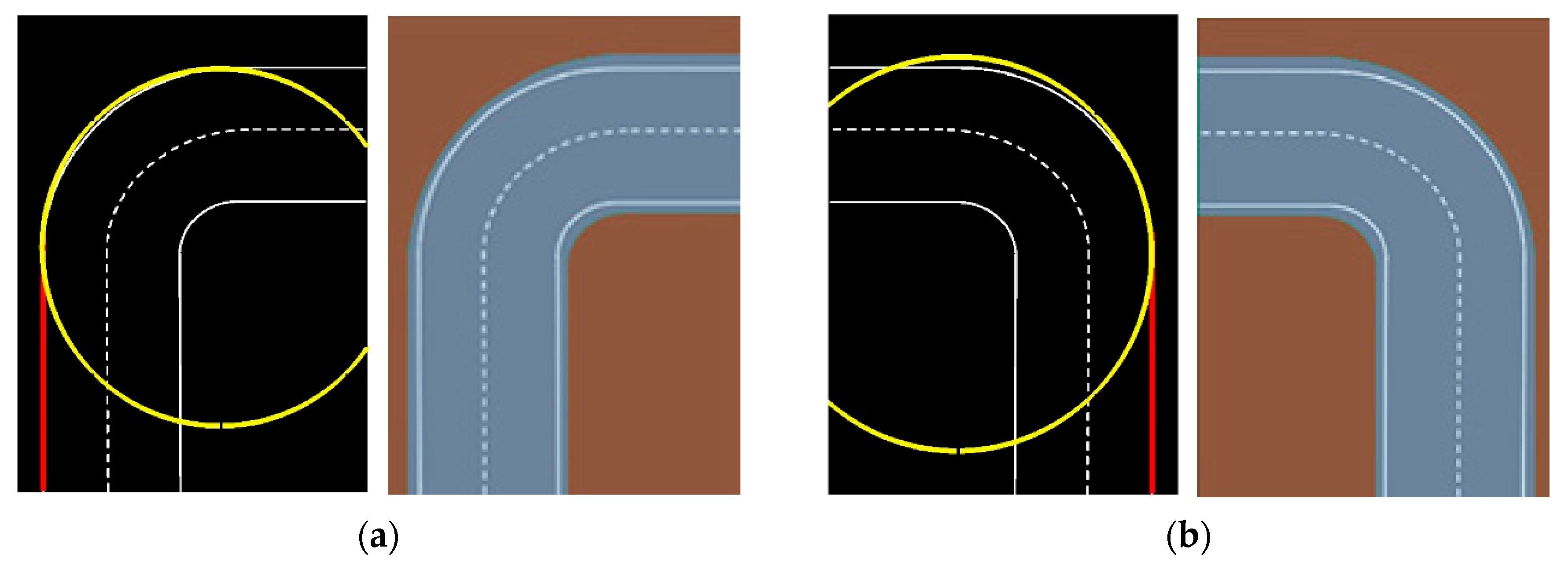
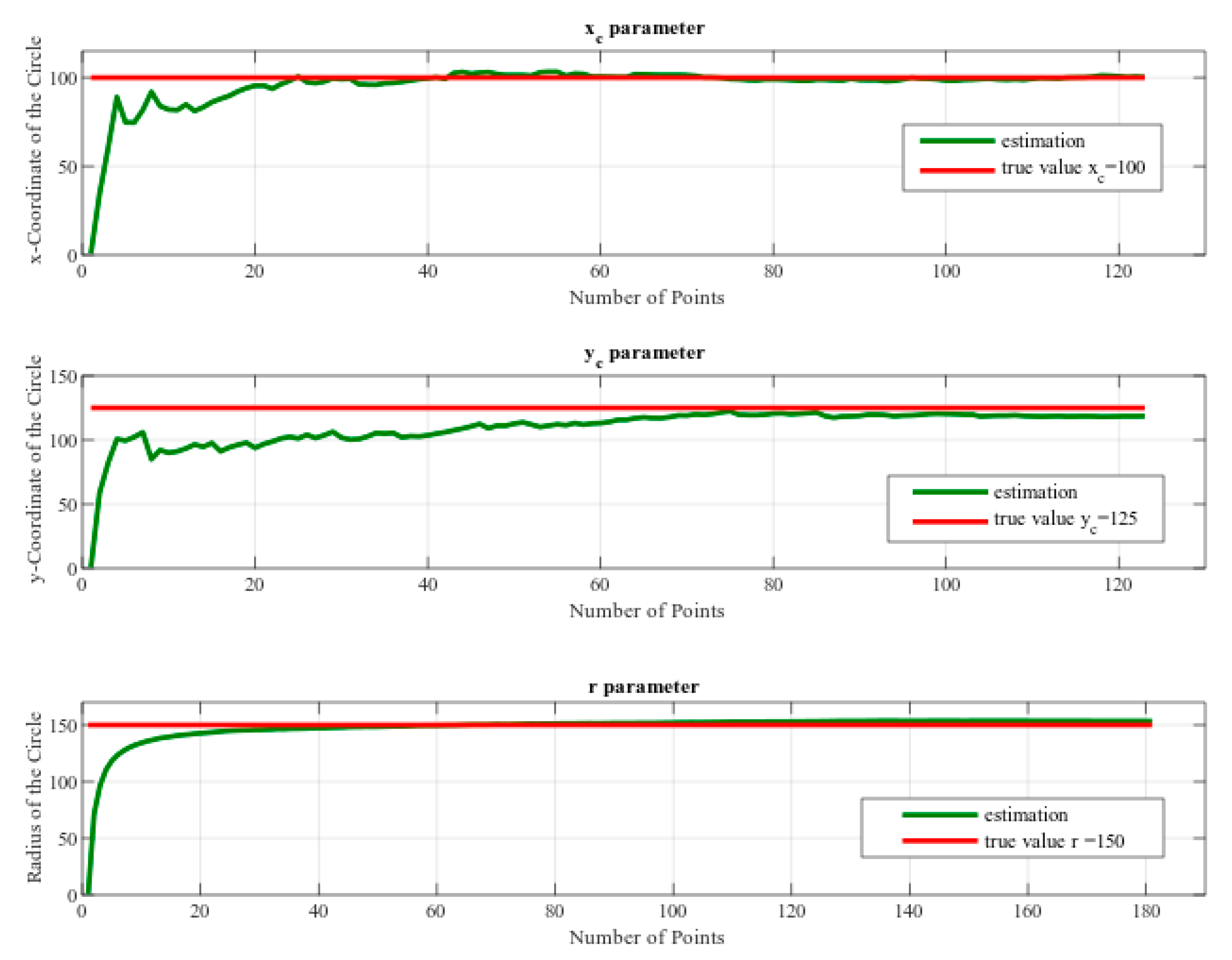
Figure 9 shows a curve lane detection expected result of Kalman filter in the prepared road image [35], this image has a circle shape road turning. The results present good performance for both of them, left turning and right turning.

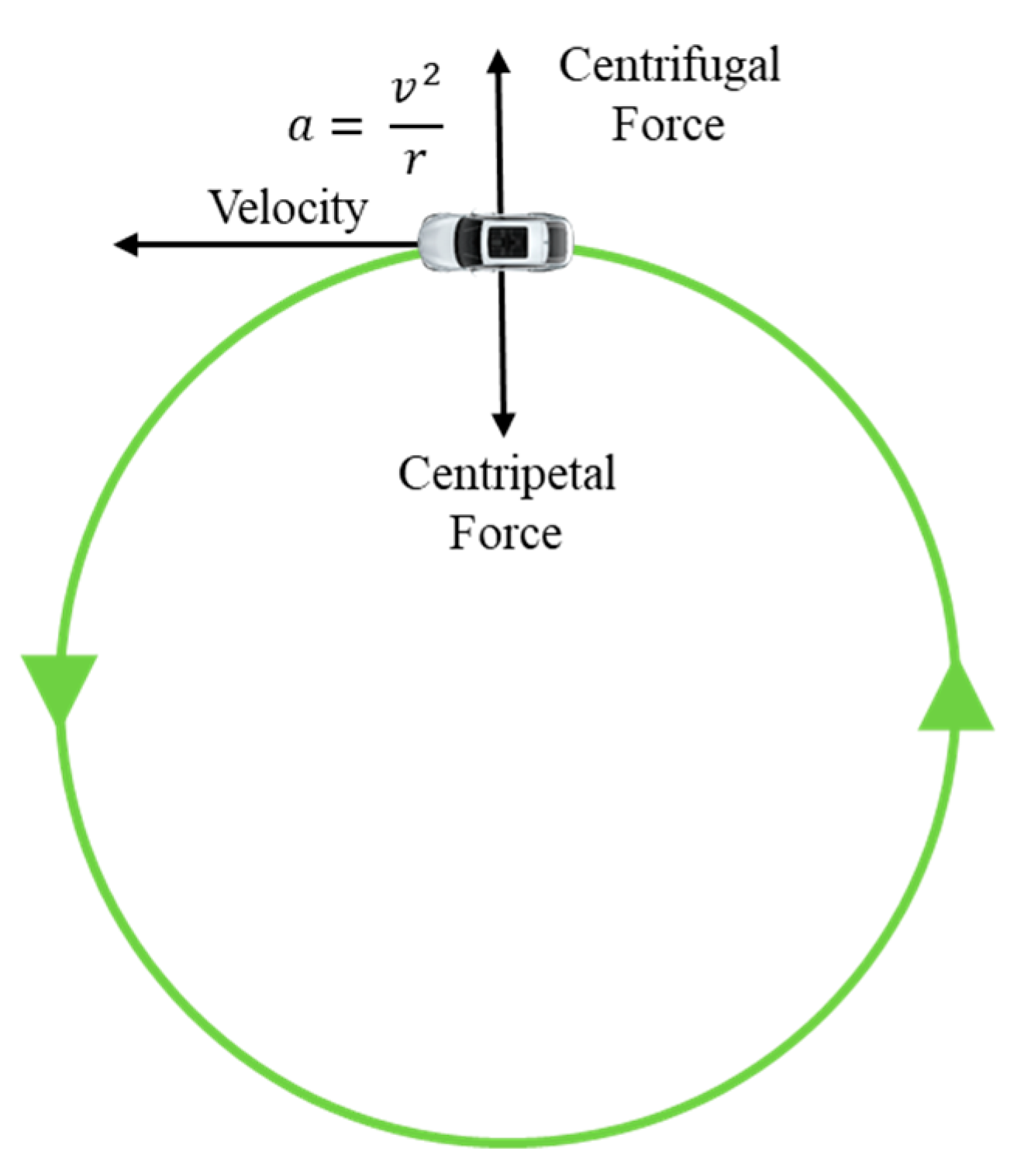
Using this result we can predict road turning and based on this value of radius we can control the speed of the self-driving car. For example, if the radius value is low, the self-driving car needs to reduce speed, if the radius value is high, the self-driving car can be on the same speed (no need to reduce speed). Also using radius value we can estimate suitable velocity based on centrifugal force Equation (33), as shown in Figure 10.

$$F_c=m\frac{u^2}{r}; u=\sqrt{\frac{F_c·r}{m}}$$

(33)

3. Setup for Simulation in 3D Environments and Results

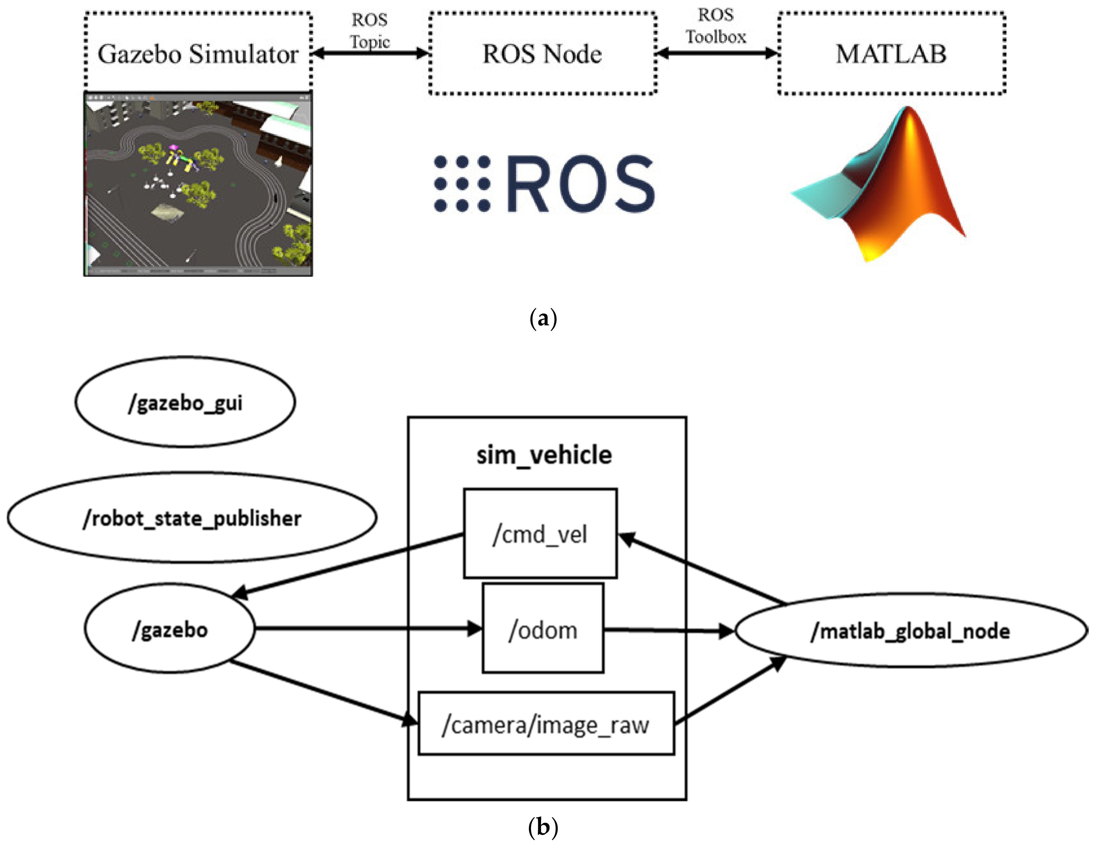
The 3D lane detection environment for simulation is designed using the GAZEBO simulator. MATLAB is used for image preprocessing, lane detection algorithm, and closed-loop lane keeping control, shown in Figure 11a. It shows the software communication in brief.

Figure 11b shows the comprehensive connection between nodes and topics in the gazebo simulator. From the gazebo GUI, the camera sensor node gives us the image_row topic. The Matlab node receives the raw RGB image of the lane and processes the frames. Then, the Matlab node generates the heading angle and sends it using cmd_vel topic to the gazebo. In order to get the trajectory of the robot, the odom topic is used to plot the position of the vehicle.

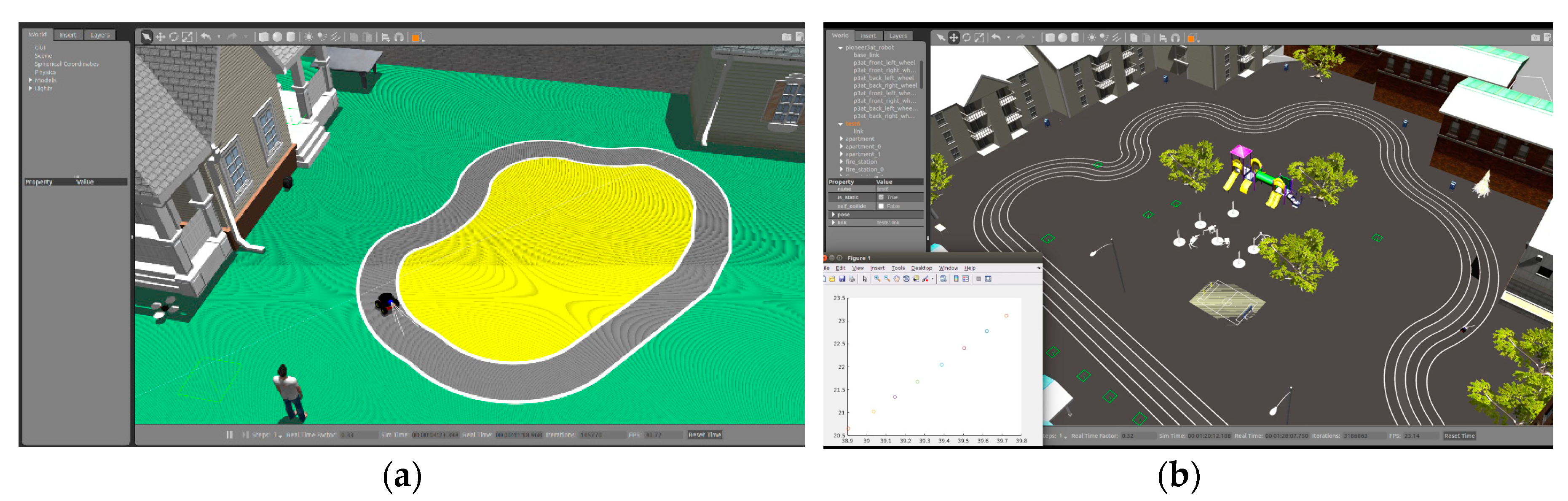
For lane detection and closed-loop lane keeping control, we used two simulated track environments using pioneer robot-vehicle as shown in Figure 12. Using this image input from the Gazebo simulator, the algorithm detects the lane and estimates the vehicle’s angular velocity and linear velocity based on lane detection results and output in Matlab. Initial parameters are set according to the simulation environment. For top view transformation, parameters are set as $H=59, f=0.01, \alpha =0.62, {\theta }_v=0.9, {\theta }_h=1.1$, and to get the binary image of the lane, the auto threshold for each channel is used. $Thres{h}_{average}=0.5804$.

To assess the viability of the introduced algorithms, random noises were added with real values. We performed the experiment with noisy measurement data of the parabola equation in Matlab. Figure 12b illustrates the 3d view and map of the athletic field and Figure 12a illustrates another track environment. The plotted graph of the trajectory path is generated from the odometry data of the robot-vehicle which shows that the curve lane follows the road curve scenario, as shown in Figure 13a,b with respect to the lane tracking of environments from Figure 12a,b.

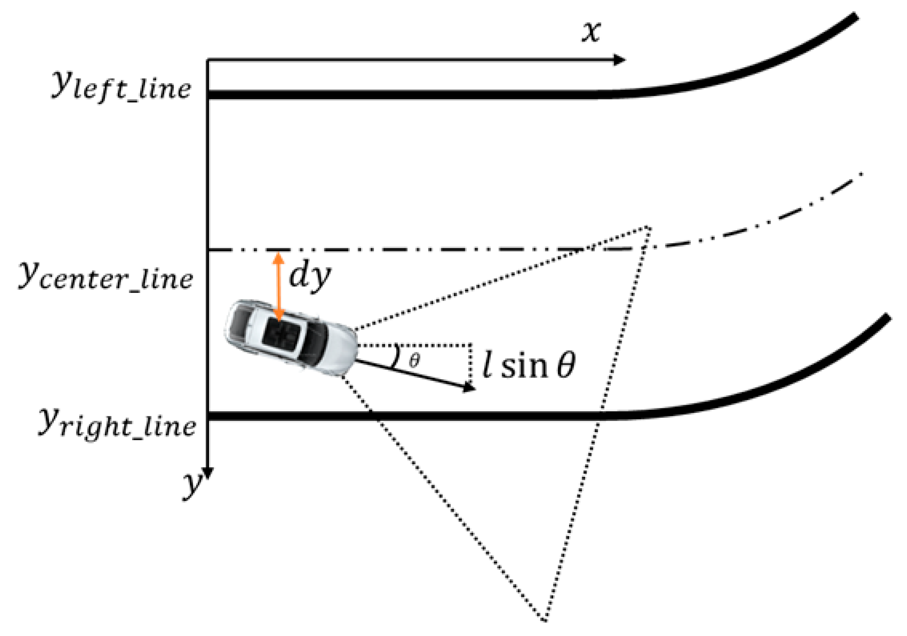
The angular velocity control uses a proportional-integral-differential (PID) controller, which is a control loop feedback mechanism. In PID control, the current output is based on the feedback of the previous output, which is computed to keep the error small. The error is calculated as the difference between the desired and the measured value, which should be as small as possible. Two objectives are executed, keeping the robot driving along the centerline $dy=0$ and keeping the robot heading angle, $\theta =0$, as shown in Figure 14. The equation can be expressed as $y_{center\_line}=\left(y_{righ{t}_{line}}+y_{lef{t}_{line}}\right)/2; dy=y_{center\_line}-y_{center\_pixel}$ from where error term can be written as $error=-\left(dy+l\sin \theta \right).$ The steering angle of the car can be estimated using a straight line detection result while also detecting the curve lanes.

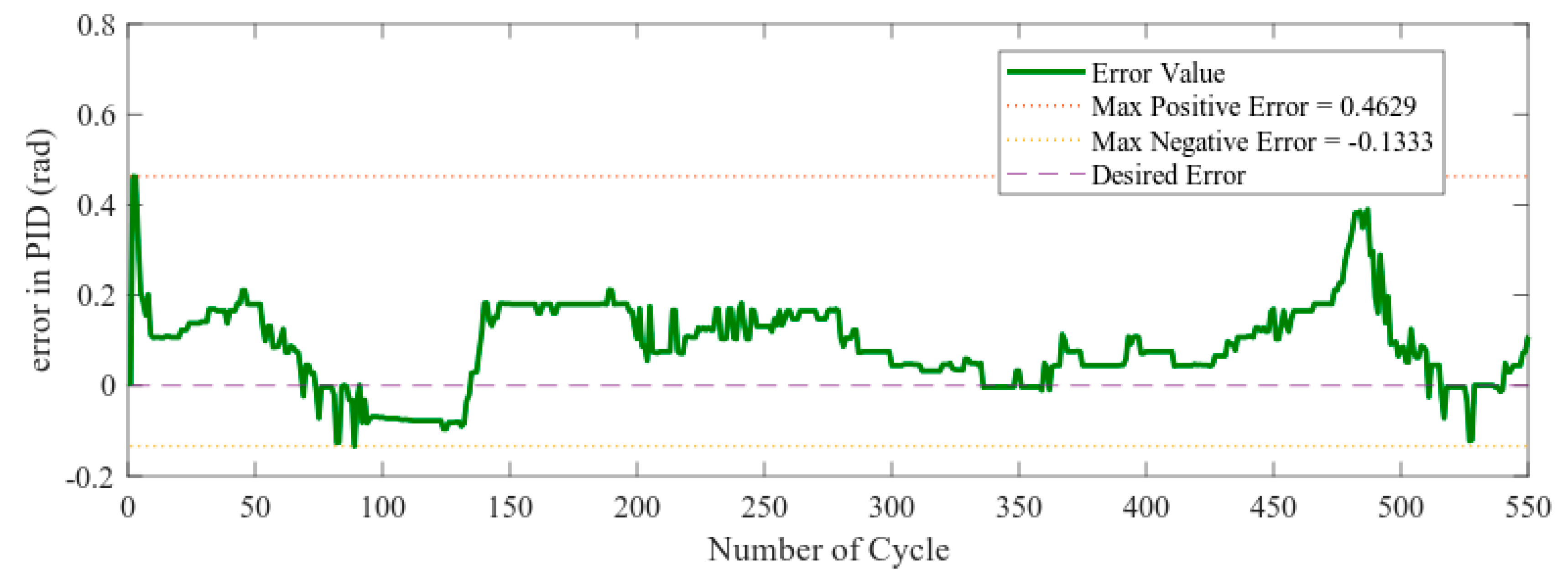
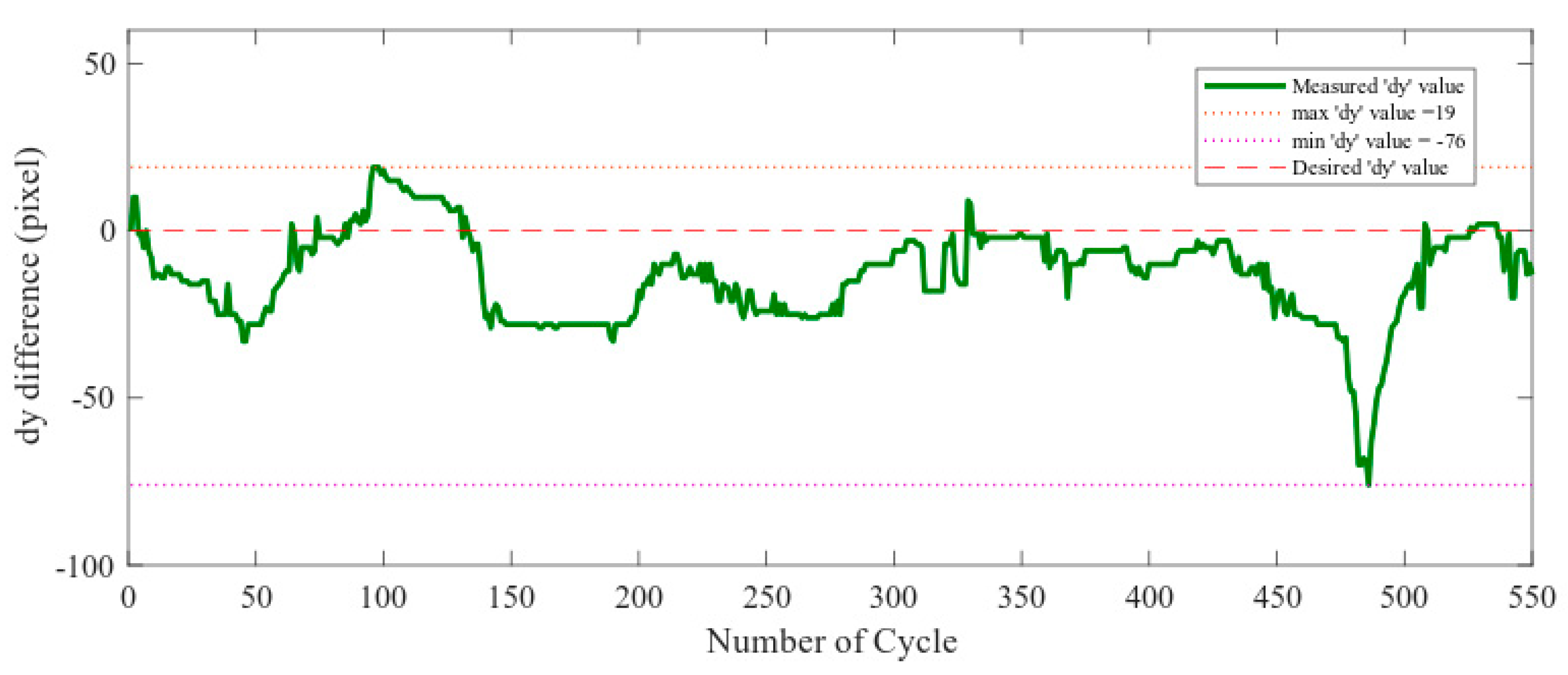
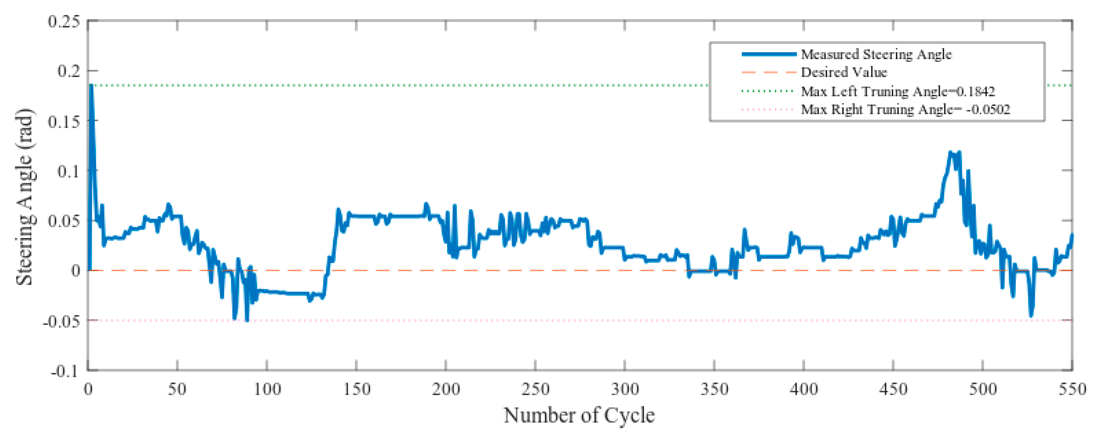
Figure 15 and Figure 16 show the PID error and $dy$ difference in pixel respectively. The steering angle is derived from the arctangent of the centerline of the vehicle. Here, co-efficient of p-term = 0.3 and co-efficient of d-term = 0.1. Figure 17 shows the steering angle in the simulation experiment in scenario one. Figure 15 shows that most of the time the error is positive. As a result, Figure 17 generates positive steering angles most of the time which means steering left. All the figures below are the result of the simulation from the map of Figure 13a. The vehicle maneuver was performed counter-clockwise. To stay in the center lane, the vehicle needs to take steering on the left. So, that is the reason for error value were greater than zero during the simulation. The portion where the error value is less than zero indicates steering right and also indicates that there is curve going right particularly at that time. The sudden reason for the spike in 480th number of cycle indicates that the $dy$ value becomes high at that moment. In order to reduce the $dy$ value and bring the vehicle to the position close to the center line, the error value is increased. Therefore, there steering angle to turn left was higher than its average value.

4. Experimental Results for the Curve Lane Detection

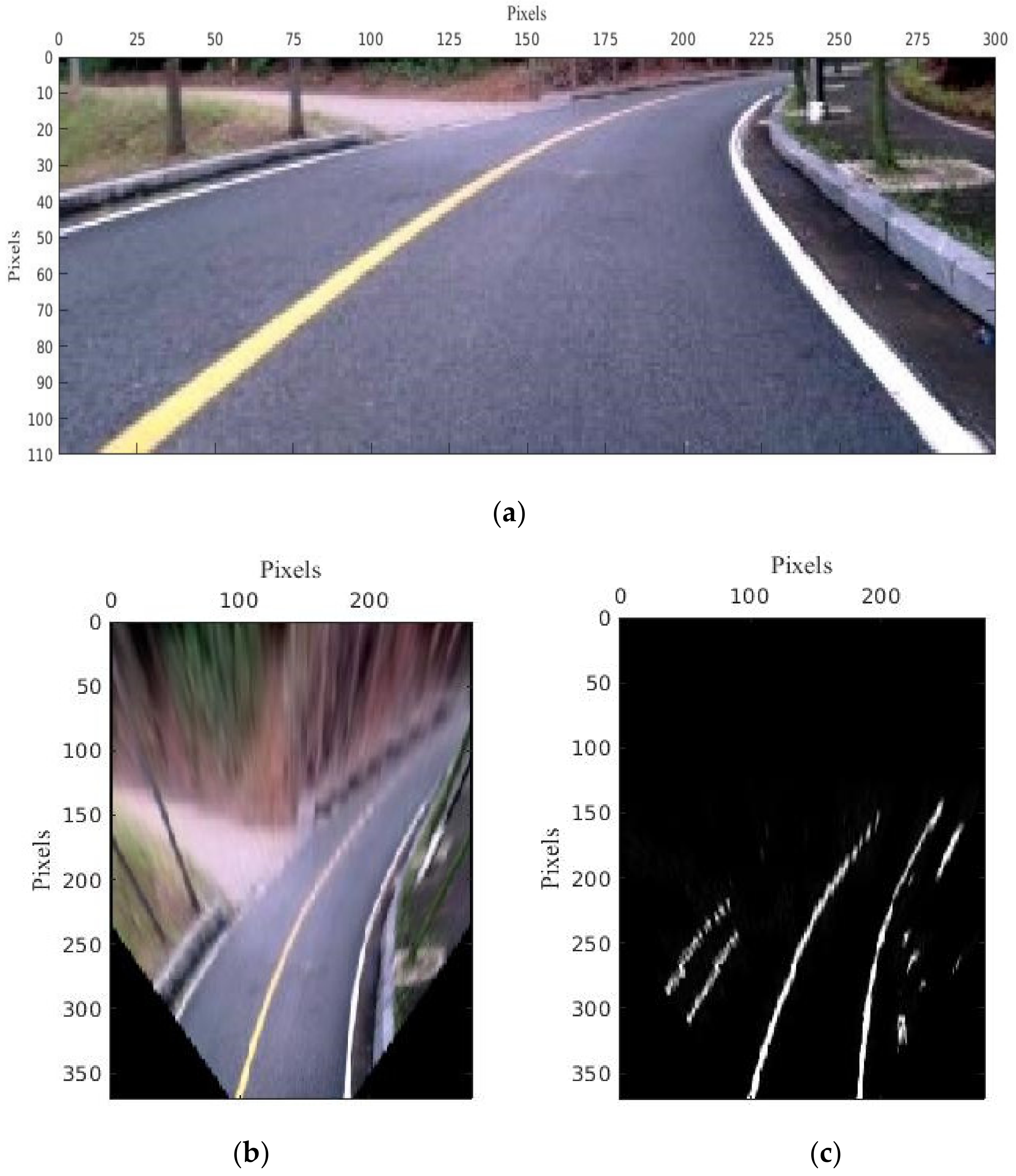
Figure 18 represents an image output from MATLAB in the pixel coordinate system in the algorithm. The image frame generated from the camera on the center is converted to a pixel coordinate system due to convenience.

Results of the auto threshold by Otsu are shown in Figure 19b from the output of the Figure 20a. For manual threshold $Thres{h}_{red}=0.7491, Thres{h}_{green}=0.7202, Thres{h}_{blue}=0.5834$ are used. $Thres{h}_{red}=0.75, Thres{h}_{green}=0.68, Thres{h}_{blue}=0.6$ are obtained from here from auto threshold values. For top view transformation, parameters are set as $H=105, f=0.01, \alpha =1.0472, {\theta }_v=0.9, {\theta }_h=1.1$.

The auto threshold results in Figure 19b are clearer than the manual threshold results in Figure 19a. Also, it can be robust in outside experiments. Top view transformation converts from pixels in the image plane to world coordinates metric as shown in Figure 20.

The Hough transform result generates lines that should be almost parallel, as shown in Figure 21. Also, the section to track the curve lane starts at the finishing point of these two longest straight lines.

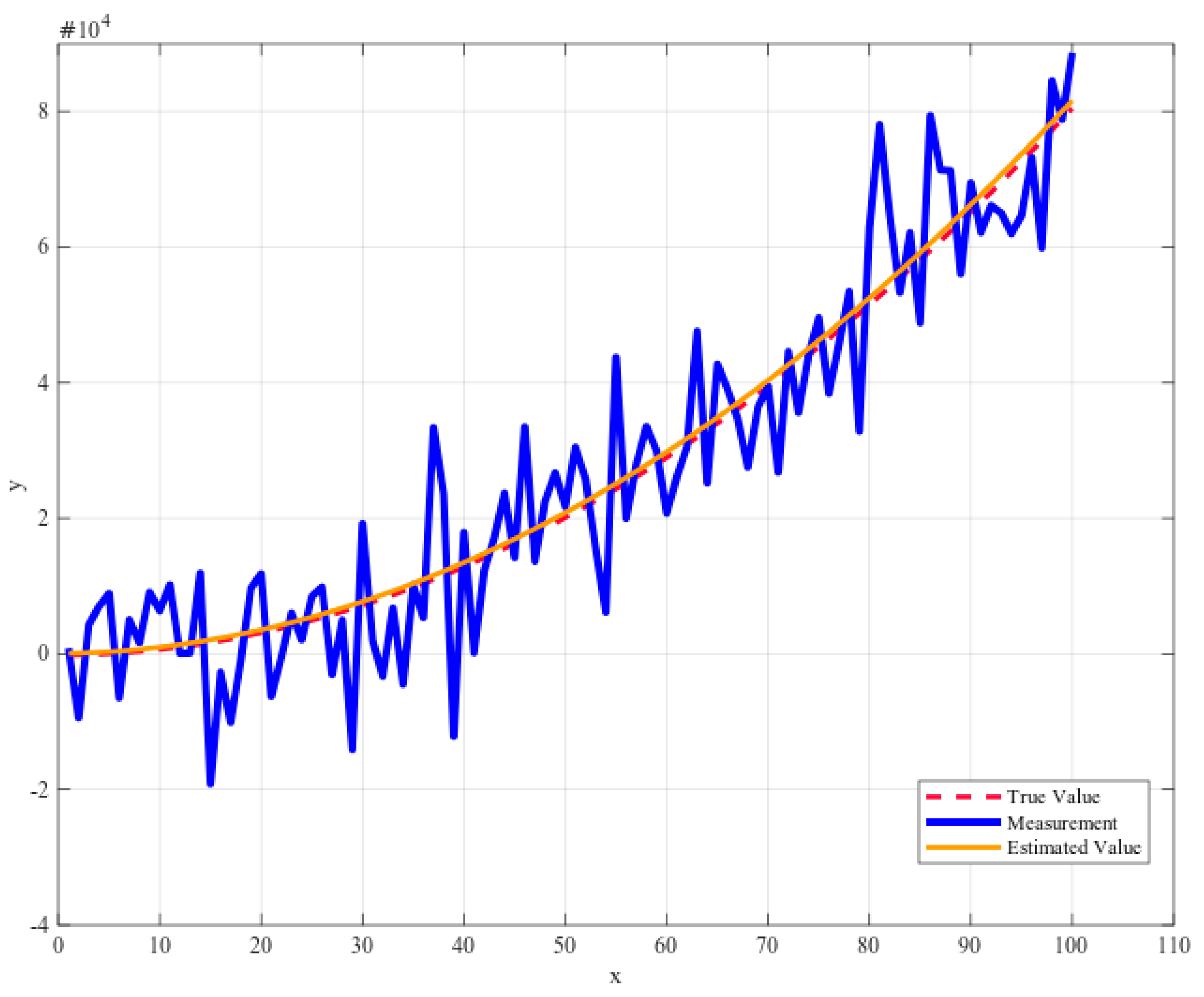
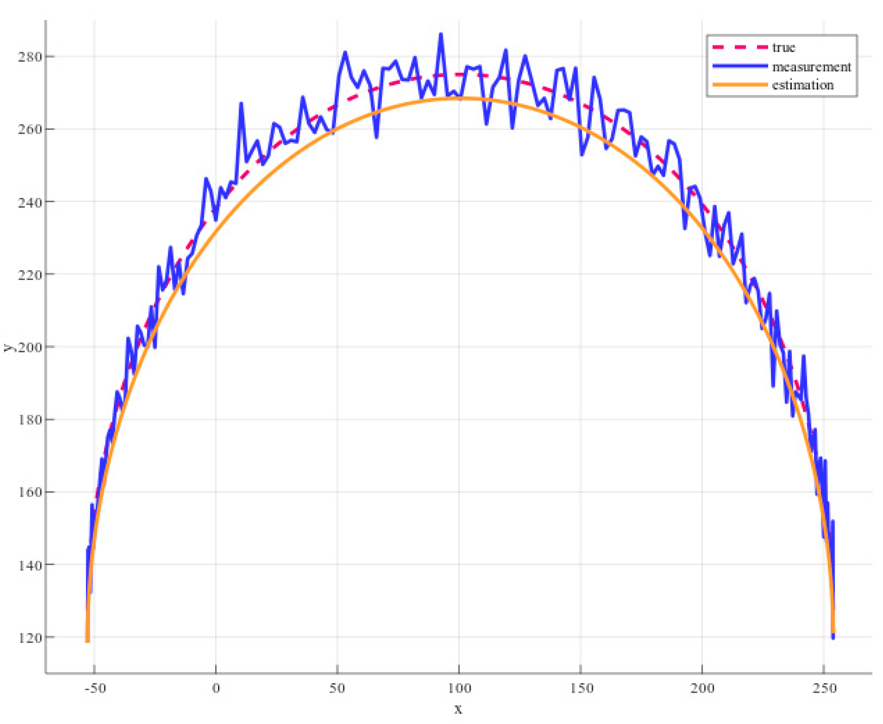
To evaluate the effectiveness of the proposed algorithms, we tested with noisy measurement data of the parabola equation in Matlab. The noisy data is created by adding random value to the true value generated using the random function from Matlab. The measurement legend marked in blue in Figure 22, is the combination of true value and noisy value. Our Kalman filter can estimate parameters of the parabola equation from noisy data. Figure 22 presents a comparison between the measurement value and estimation value, the real value.

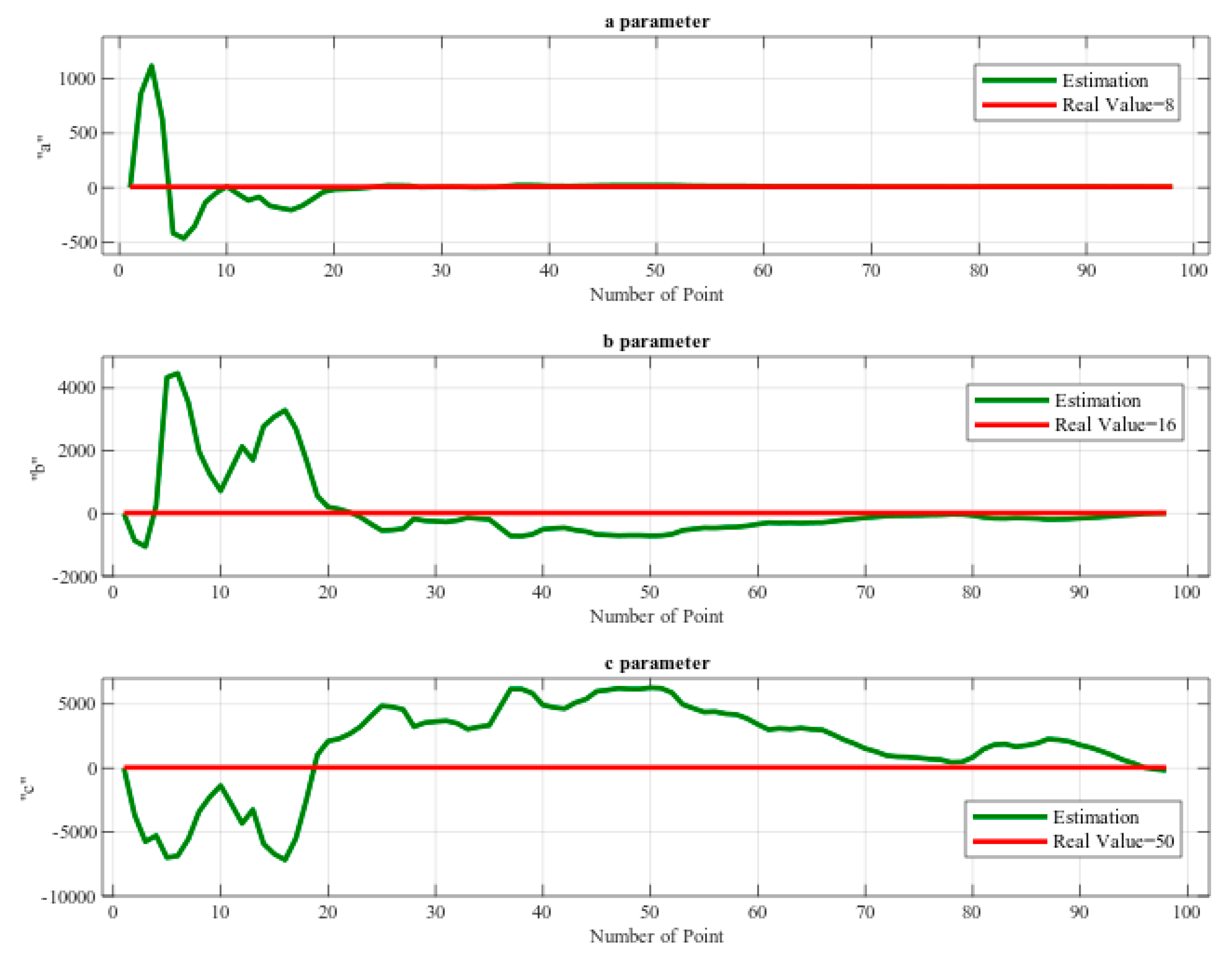
In Figure 23, the graphs illustrated the estimation results of parameters. At the end of the process, estimation results become almost equal to true values. In this simulation, “a” parameter’s true value is 8 and the estimated value is 7.4079, the “b” parameter’s true value is 16 and the estimated value is 22.4366, “c” parameter’s true value 50 and the estimated value is 37.115. There is almost no difference between the estimated value and the true value compared to the noise value ratio. Now, it is possible to apply the proposed algorithms in the processed image to perform the detection process for the curve lane.

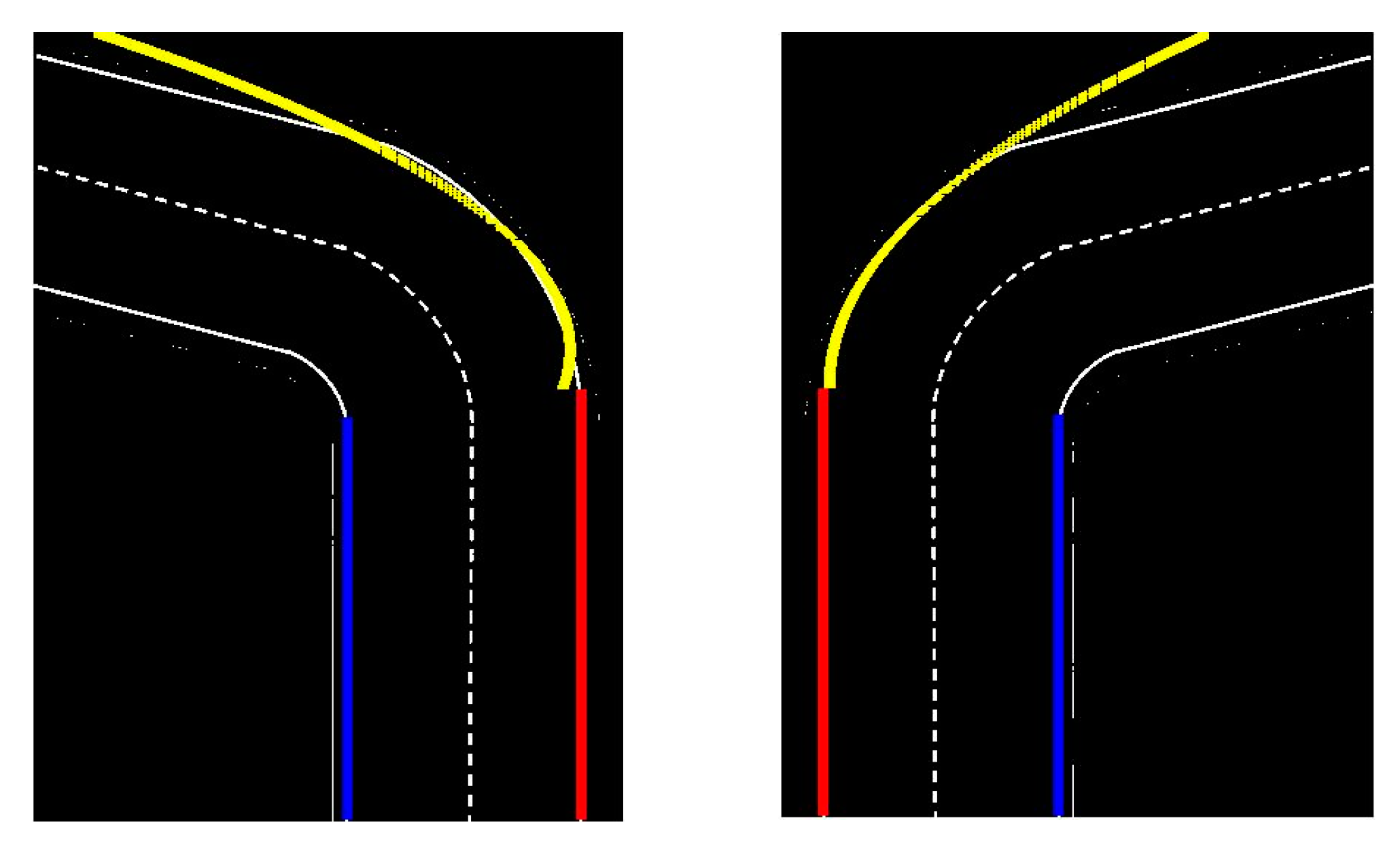
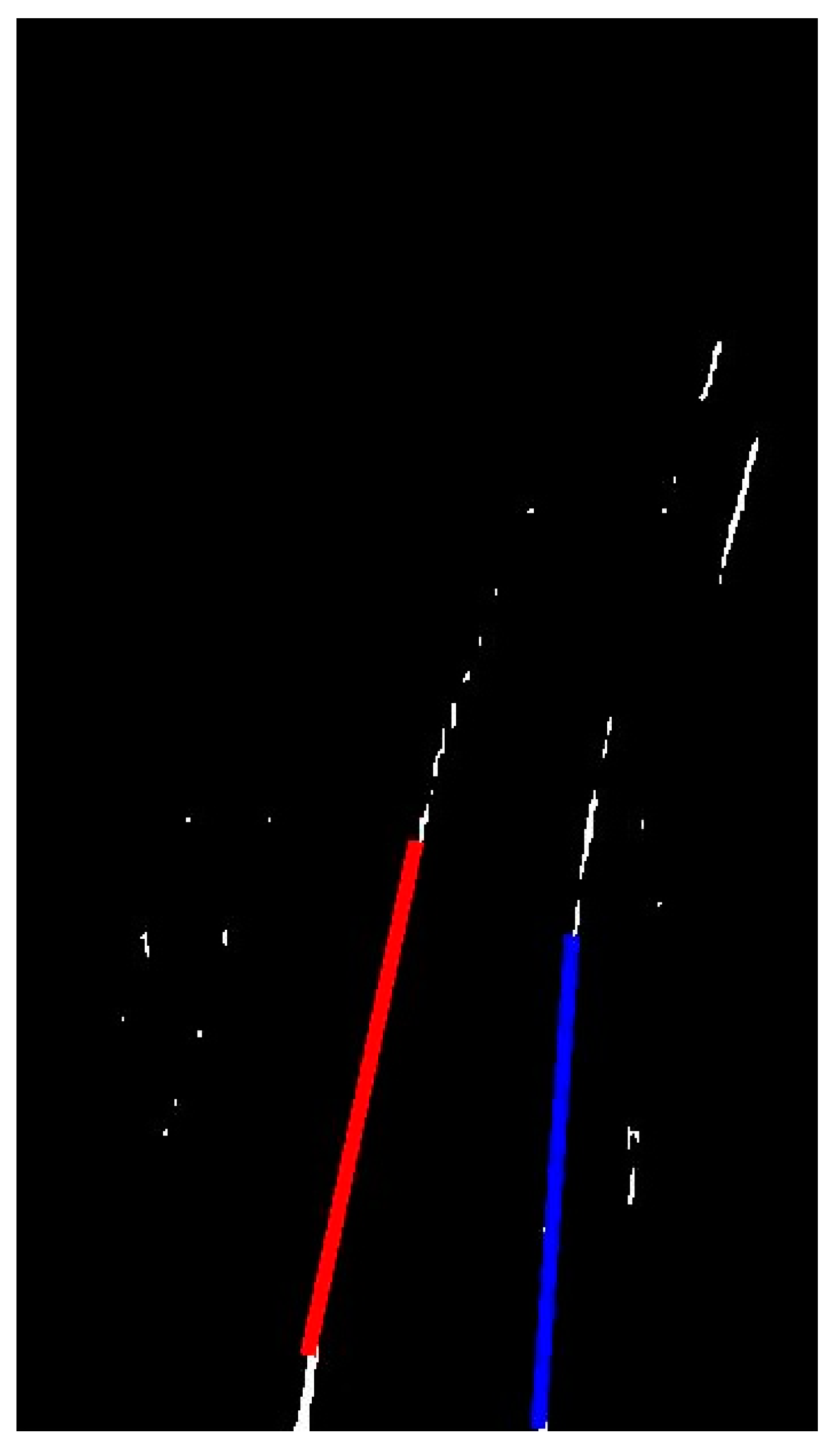
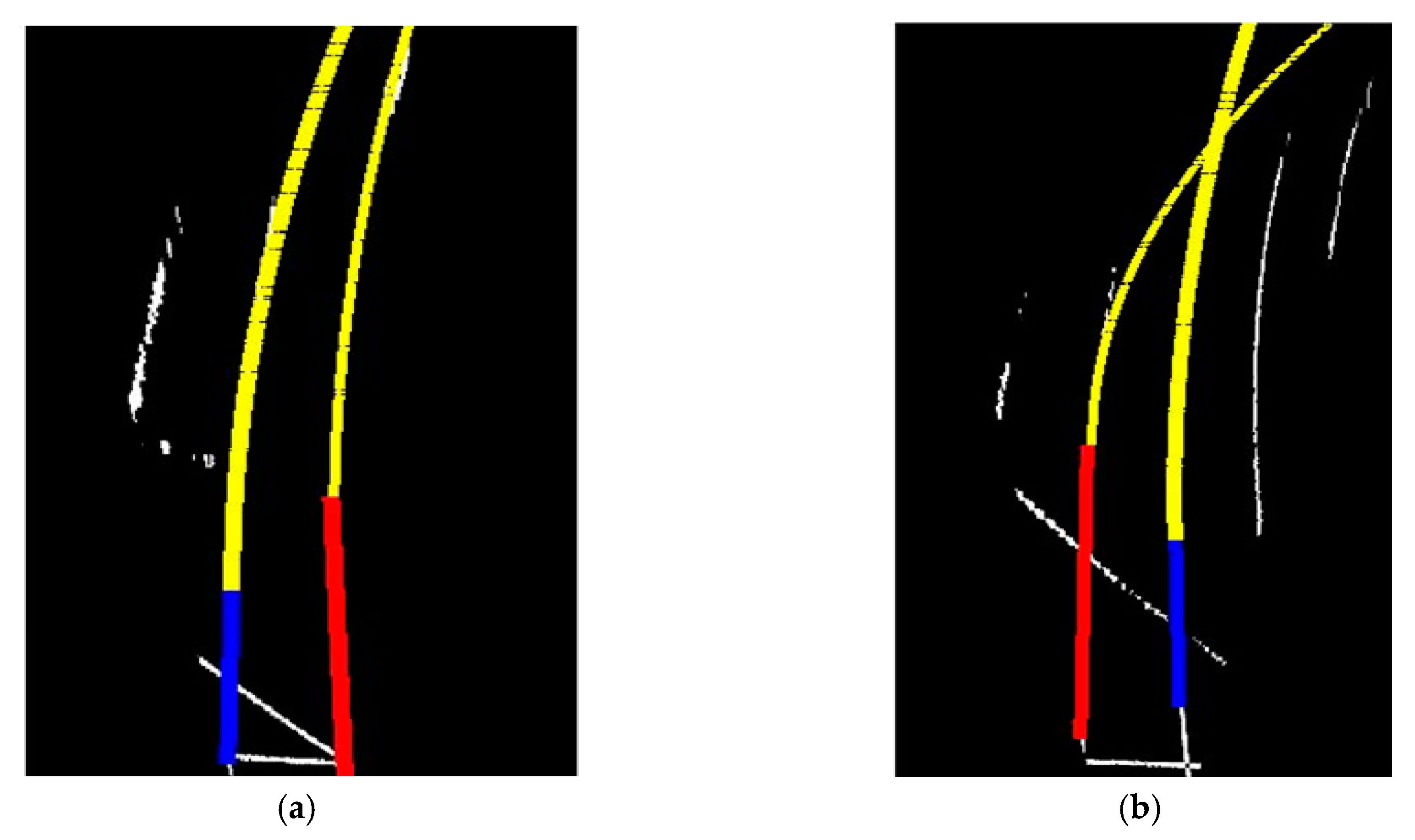
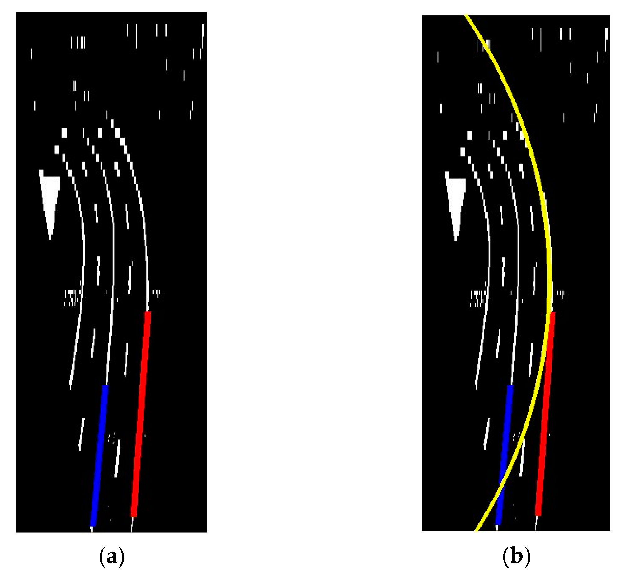
Figure 24 presents the real experimental results of the curve line detection based on the Kalman filter. Where the yellow line is the result of our algorithm and estimation results of first line $a=-1.2186·{10}^{-4}$, $b=0.8486$, c$=382.4092$, and estimation results of second line $a=-3.0639·{10}^{-5}$, $b=0.238$, c $=885$ in the first experiment image of the road. In the second experiment image of the road, estimation results of first line $a=-2.6319·{10}^{-5}$, $b=0.2096$, c $=938.96$, estimation results of the second line $a=-3.166·{10}^{-5}$, $b=0.2832$, c $=1292$. The simulation result of circle detection is shown in Figure 25. Figure 26 shows a comparison between the measurement value and the estimation value, the true value of circle detection. Of course, the proposed algorithm also has some shortcomings. For example, the right-hand side of Figure 24 is the aftermath of shadow reflection from the left side of the lane. The reflection produces brightness in the lane image, causing a slight change in the detection. Further research is needed later.

After that, we tested in the top-view transformed image of the different circular real roads. Figure 27a,b illustrates the result of curve line detection using the circle model in real road image.

Here, the yellow line is the result of our algorithm and radius $r=1708.2$, the center of the circle is $x_{center}=957.81$, $y_{center}=-1260.2$. Using this result we can predict road turning and based on this value of radius we can control the speed of the self-driving car. For example, if the radius value is low, the self-driving car needs to reduce speed, if the radius value is high, the self-driving car can be at the same speed (no need to reduce speed).

5. Conclusions

In this paper, a curve line detection algorithm using the Kalman filter is presented. The algorithm is split into two sections:

(1)

Image pre-processing. It contains Otsu’s threshold method. Top view image transforms to create a top-view image of the road. A Hough transform to track a straight lane in the near-field of view of the camera sensor.

(2)

Curve lane detection. The Kalman filter provides the detection result for curve lanes in the far-field of view. This section consists of two different methods, the first method is based on the parabola model, and a second method is based on the circle model.

The experimental results show that the curve lane detection method can be effectively detected even under a very noisy environment and with parabola and circle model. Also, we have deployed the algorithm in the gazebo simulation environment to verify the performance. One advantage of the proposed algorithm is its robustness against noise, as our algorithms are based on the Kalman filter. The viability of the proposed curve lane detection strategy can be applied to the self-driving car systems as well as to the advanced driver assistant systems. Based on our curve lane detection results, we can predict road turning, and also estimate suitable velocity and angular velocity for the self-driving car. Also, our proposed algorithm provides close-loop lane keeping control to stay in lane. The experimental result shows the proposed algorithm achieves an average of 10 fps. Even though the algorithm has an auto threshold method to adjust with different light conditions such as low-light, further study is needed to detect lane in conditions like light reflection, shadows, worn-lane, etc. Moreover, the proposed algorithm does not require high GPU processing unit to perform other CNN-based algorithms. The performance is satisfactory in the CPU-based system according to the fps. However, CNN-based study in the pre-processing step can provide a more efficient result for edge detection.