Article

Three-Dimensional Imaging via Time-Correlated Single-Photon Counting

1
State Key Laboratory for Strength & Vibration of Mechanical Structures, School of Aerospace, Xi’an Jiaotong University, Xi’an 710049, China
2
Shaanxi Engineering Laboratory for Vibration Control of Aerospace Structures, Xi’an Jiaotong University, Xi’an 710049, China
3
Electronic Materials Research Laboratory, Key Laboratory of the Ministry of Education and International Center for Dielectric Research, School of Electronic and Information Engineering, Xi’an Jiaotong University, Xi’an 710049, China
4
MOE Key Laboratory for Nonequilibrium Synthesis and Modulation of Condensed Matter, Department of Applied Physics, Xi’an Jiaotong University, Xi’an 710049, China
*
Author to whom correspondence should be addressed.
Appl. Sci. 2020, 10(6), 1930; https://doi.org/10.3390/app10061930
Submission received: 6 February 2020 / Revised: 29 February 2020 / Accepted: 6 March 2020 / Published: 11 March 2020
(This article belongs to the Section Optics and Lasers)

Abstract

:
Three-dimensional (3D) imaging under the condition of weak light and low signal-to-noise ratio is a challenging task. In this paper, a 3D imaging scheme based on time-correlated single-photon counting technology is proposed and demonstrated. The 3D imaging scheme, which is composed of a pulsed laser, a scanning mirror, single-photon detectors, and a time-correlated single-photon counting module, employs time-correlated single-photon counting technology for 3D LiDAR (Light Detection and Ranging). Aided by the range-gated technology, experiments show that the proposed scheme can image the object when the signal-to-noise ratio is decreased to −13 dB and improve the structural similarity index of imaging results by 10 times. Then we prove the proposed scheme can image the object in three dimensions with a lateral imaging resolution of 512 × 512 and an axial resolution of 4.2 mm in 6.7 s. At last, a high-resolution 3D reconstruction of an object is also achieved by using the photometric stereo algorithm.

1. Introduction

In recent years, single-photon counting lidar has been widely used in three-dimensional (3D) imaging under weak light conditions because of its single-photon sensitivity and picosecond time resolution. This technology has many significant applications, such as long-distance imaging, underwater target detection [1]. The core idea of this technology is time-correlated single-photon counting (TCSPC). TCSPC is the most effective way to measure the temporal structure of weak optical signals, which is based on the accurate measurement of photon arrival times and time difference [2,3]. TCSPC was mainly used in the detection of fluorescence lifetime in the early stage [4,5,6,7,8,9,10,11,12]. After that, TCSPC began to be used in the field of laser ranging [13,14,15,16,17,18] and gradually developed to the direction of laser long-distance 3D imaging based on time-of-flight (TOF) algorithm [19,20,21,22,23,24,25,26]. Recently, Li et al. achieved the imaging of targets 45 kilometers away [27]. Kirmani et al. [28] and Xialin Liu et al. [29] detected the first photon in TCSPC system to image the object.
In the general TCSPC system, the image result is greatly affected by environmental noise because of the ultra-high sensitivity of the single-photon detectors (SPD). Up to now, most of the research teams used the range-gated technology to decrease the impact of noise [20,24,27]. Besides, Kong et al. used two Geiger-mode avalanche photodiodes and an AND gate to reduce false alarms caused by environmental noise [30]. Huang et al. come up with a new method to decrease environmental noise by using correlative photons and spatial correlations [31].
In this paper, we combine SPD, high repetition rate laser pulses illumination and TCSPC technology to design a new imaging scheme. The new scheme has the capability of de-noise, high-resolution imaging, accurate analysis of the photon flight time and 3D imaging. Three experiments are completed to demonstrate the power of the new imaging scheme. The first is the de-noise experiment which proves that our scheme can image the object when the signal-to-noise ratio (SNR) is decreased to −13 dB and improve the structural similarity index (SSIM) [32] of imaging results by 10 times. The second proves that the scheme has a lateral imaging resolution of 512 × 512 and an axial resolution of 4.2 mm. The third is 3D imaging by photometric stereo algorithm which uses multiple detectors to reconstruct the 3D image of the object. Besides, the new imaging scheme has the potential to realize turbulence-free imaging [33], non-of-sight imaging technology [34] and imaging in a complicated environment.

2. Theory Analysis

In our scheme, the core idea is to use the TCSPC technology to get the information of the number and arrival time of each signal photon. Aided by the range-gated technology, the environmental noise can be significantly reduced. Furthermore, with these information the TOF algorithm and photometric stereo algorithm can be used to reconstruct the 3D model of the object.

2.1. TCSPC

TCSPC technology, which is mainly used to detect the low intensity and high repetition frequency pulsed laser, is developed on the basis of the photon-counting technology. The realization process is as follows: pulse laser emits a pulse, and a synchronization signal is generated at the same time to trigger the START of the TCSPC module to start timing, as shown in Figure 1a. Each photon detected by the SPD triggers the STOP of the TCSPC module to stop timing. Then the TCSPC module can record the arrival time of each photon reference to the emitted laser pulse. At last, after statistical processing, the histogram of the number of photons VS the arrival time can be obtained, as shown in Figure 1b.

2.2. Detection Probability of Signal Photon Events

As described in [28,35], supposing the object point ( x , y ) is illuminated by a pulse S ( t ) and the echo pulse reflected the SPD is S t 2 z x , y c . Then the theoretical number of photons detected by SPD is
r x , y ( t ) = α x , y S t 2 z x , y c + b ,
where z x , y represents the flight distance of the laser from the target point, c represents the speed of light, α x , y represents the reflectivity of target and b represents the number of background photons. Considering that the quantum efficiency of SPD is η and the dark counts are d, the actual number of photons λ x , y detected by the SPD is
λ x , y ( t ) = η r x , y ( t ) + d = η α x , y S t 2 z x , y c + ( η b + d ) .
Let the pulse laser period be T r , then the average number of photons received by the SPD in a period is
λ x , y = λ x , y ( t ) · T r = η α x , y 0 T r S ( t ) d t + ( η b + d ) T r = η α x , y S + B .
According to the Poisson probability model [36], for each pulse emitted by the laser, the number of photons k received by the detector satisfies the following distribution:
P x , y ( n = k ) = λ x , y k k ! e λ x , y .
When the SPD does not record any photon, that is k = 0 , the probability can be denoted by P x , y ( n = 0 ) = e λ x , y .

2.3. Imaging Scheme Based on TCSPC

In our scheme, the dead time of SPD is longer than the pulse width of laser. Therefore, the number N x , y of photons received by the SPD after each point scanned by the scanning mirror is
N x , y = 1 ω T r 1 e λ x , y ,
where T r denotes the pulse laser period and ω denotes the scanning frequency of scanning mirror. The pixel value of target point ( x , y ) is represented by N x , y . When the whole object is scanned by the scanning mirror, the two-dimensional image of the target can be obtained by rearranging the pixel values. Besides, because the flight time of each photon and the number of photons can be obtained accurately by the TCSPC module, the depth information of the object can be calculated by the TOF algorithm. Lastly, multiple SPDs are used to detect objects from different angles. By combining the photometric stereo algorithm, we can also get the 3D model of the object.

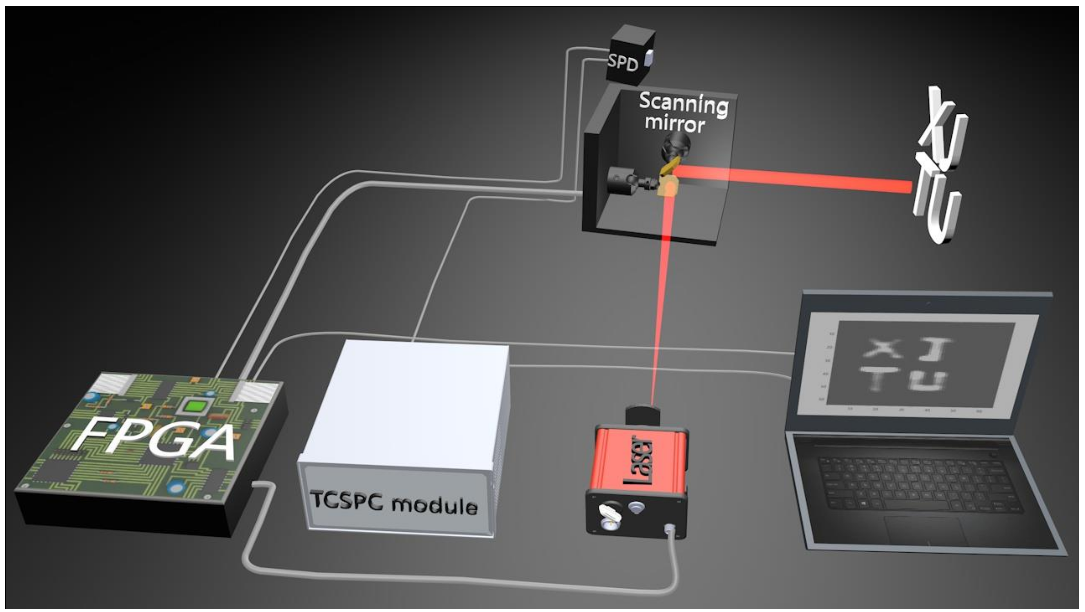
3. Experimental Setup and Results

To verify the 3D imaging scheme based on TCSPC proposed in this paper, three groups of experiments are performed to confirm the de-noise ability, high-resolution imaging ability, 3D imaging based on the photometric stereo algorithm. We use a pulsed laser with a wavelength of 532 nm as light source, which generated 30 ps duration pulses at a repetition rate of 10 MHz. The SPD module is the PDM series manufactured by Micron Photon Devices. The dead time of SPD is 80 ns and the quantum efficiency at 532 nm is about 45%. Besides, HydraHarp 400, whose time resolution down to 1 ps and maximum count rate of up to 12 Mcps per channel, is used as the TCSPC module and a field-programmable gate array (FPGA) is used as the main controller.

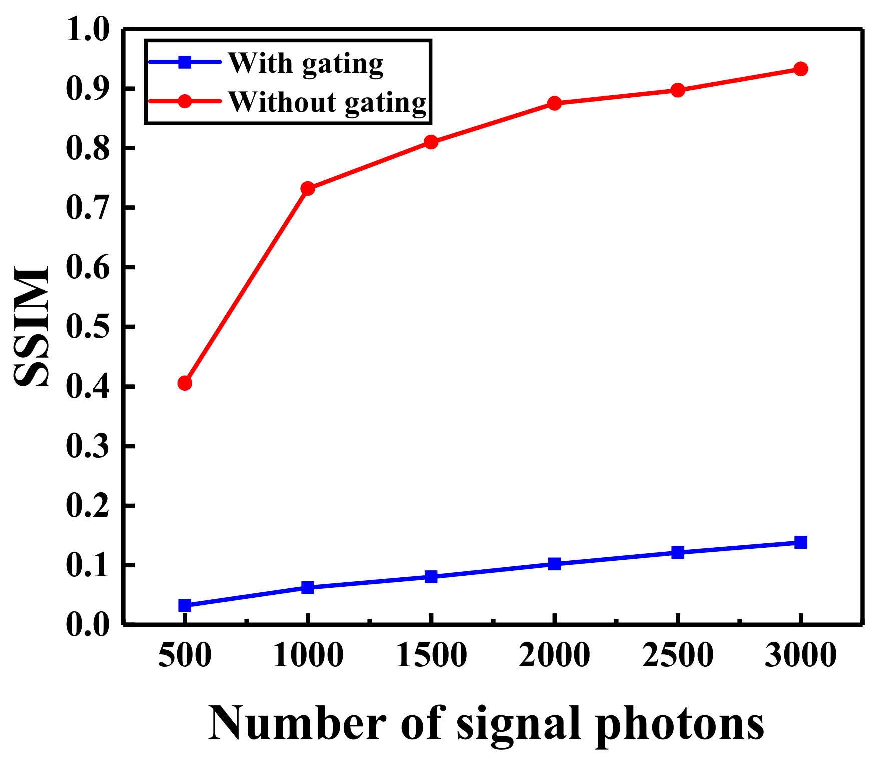
3.1. Noise Reduction Experiment Based on Range-Gated Technology

The experimental setup is depicted in Figure 2. FPGA controls the laser to emit a pulse and simultaneously generates a synchronous signal input to the HydraHarp 400 to trigger the START signal to start timing. After each fixed number of pulses produced by the laser (1024 pulses in our experiment), FPGA controls the scanning mirror to rotate once. Then SPD records the corresponding photon signal. Since the pulse width (30 ps) of the laser is smaller than the dead time of SPD (80 ns), the SPD can only respond to one photon at most for each pulse. So the probability that SPD detects the signal light is as shown in Equation (5). After the entire object is scanned by the scanning mirror, the computer can get the image of the object by rearranging the photon signals of HydraHarp 400 according to the preset scanning mode of scanning mirror.
The experimental results are shown in Figure 3. During the experiment, the number of noise photons in the environment is kept at around 10,000 counts per second (cps), and the number of signal photons is decreased from 3000 cps to 500 cps in turn. The experimental results are compared between the imaging results with and without the range-gated technology. As shown in Figure 3, the experimental image quality with gating is obviously better than that without gating. When the number of signal photons decreased to 500 cps, that is SNR is −13 dB, the experimental results with gating can still distinguish the object while the image without gating cannot. Besides, the SSIM, defined as Equation (6), is used to evaluate the qualities of the reconstructed images.
SSIM ( x , y ) = 2 μ x μ y + C 1 2 σ x y + C 2 μ x 2 + μ y 2 + C 1 σ x 2 + σ y 2 + C 2 ,
where μ x , μ y , σ x , σ y and σ x y are the local means, standard deviations, and cross-covariance for images x , y . Furthermore, C 1 = ( 0.01 × L ) 2 , C 2 = ( 0.03 × L ) 2 , where L is the specified dynamic range value (10 bits in this experiment). As shown in Figure 4, the SSIM of reconstructed images with gating is 10 times higher than that without gating.

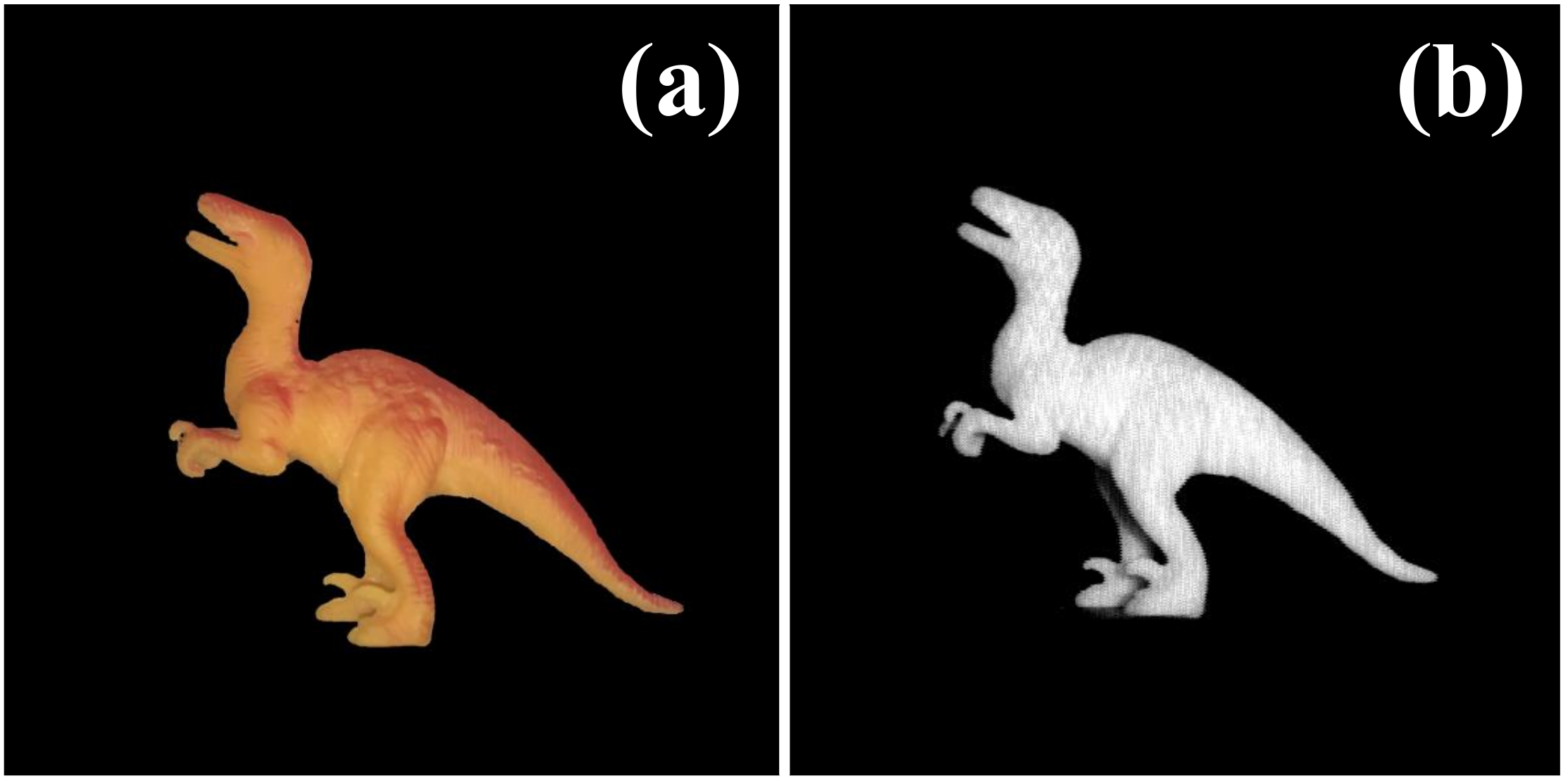
3.2. High-Resolution Imaging Experiments for Complex Objects

In this part, two sets of experiments are set to verify the high resolution including the lateral resolution and the axial resolution of the scheme. Firstly, the lateral resolution of our scheme can be calculated by
R = 1.22 λ z D 0 0 . 5 mm ,
where λ is the wavelength of the laser, D 0 is beam waist diameter of laser, z is the distance from the target to laser. To further prove the lateral resolution, we choose a dinosaur model with a size of 8 cm × 6 cm × 2 cm as the imaging object in this experiment. The experimental process is roughly the same as that of the experiment in Section 3.1. Figure 5 shows the original object and the experimental imaging result, in which the image resolution of the object is 512 × 512 , the image depth is 8 bit and the time for one frame is about 6.7 s.
Then to ensure the axial resolution, a whiteboard ( 5 cm × 5 cm ) is placed on the stepper motor (TSA150-B, repeat positioning accuracy less than 7 um). The stepper motor moves ten times and moves 10 mm each time. The distance that the whiteboard moves is evaluated by the TOF algorithm, defines as:
D = 1 2 c × Δ t ,
where D is the distance, c is the speed of light and Δ t is the time interval. In this experiment, the theoretical total time jitter mainly consists of the pulse width of the laser ( t pulse 30 ps ) , the time jitter of TCSPC module ( t TCSPC 12 ps ) and the time jitter of SPD t SPD 50 ps , as the function of
T σ = t pulse 2 + t TCSPC 2 + t SPD 2 60 ps .
As shown in Figure 6a, the total time jitter measured by the experiment is 90 ps. Therefore the distance error D σ of our scheme is D σ = 1 / 2 × c × T σ 13.5 mm . Because we take the average value of 10 points near the peak position as the measurement value each time, the actual measurement error D ¯ σ can be decreased to 4.2 mm, as the function:
D ¯ σ = D σ / N .
Figure 6b shows the measurement results and Figure 6c shows the measurement errors which are less than ±1.5 mm.

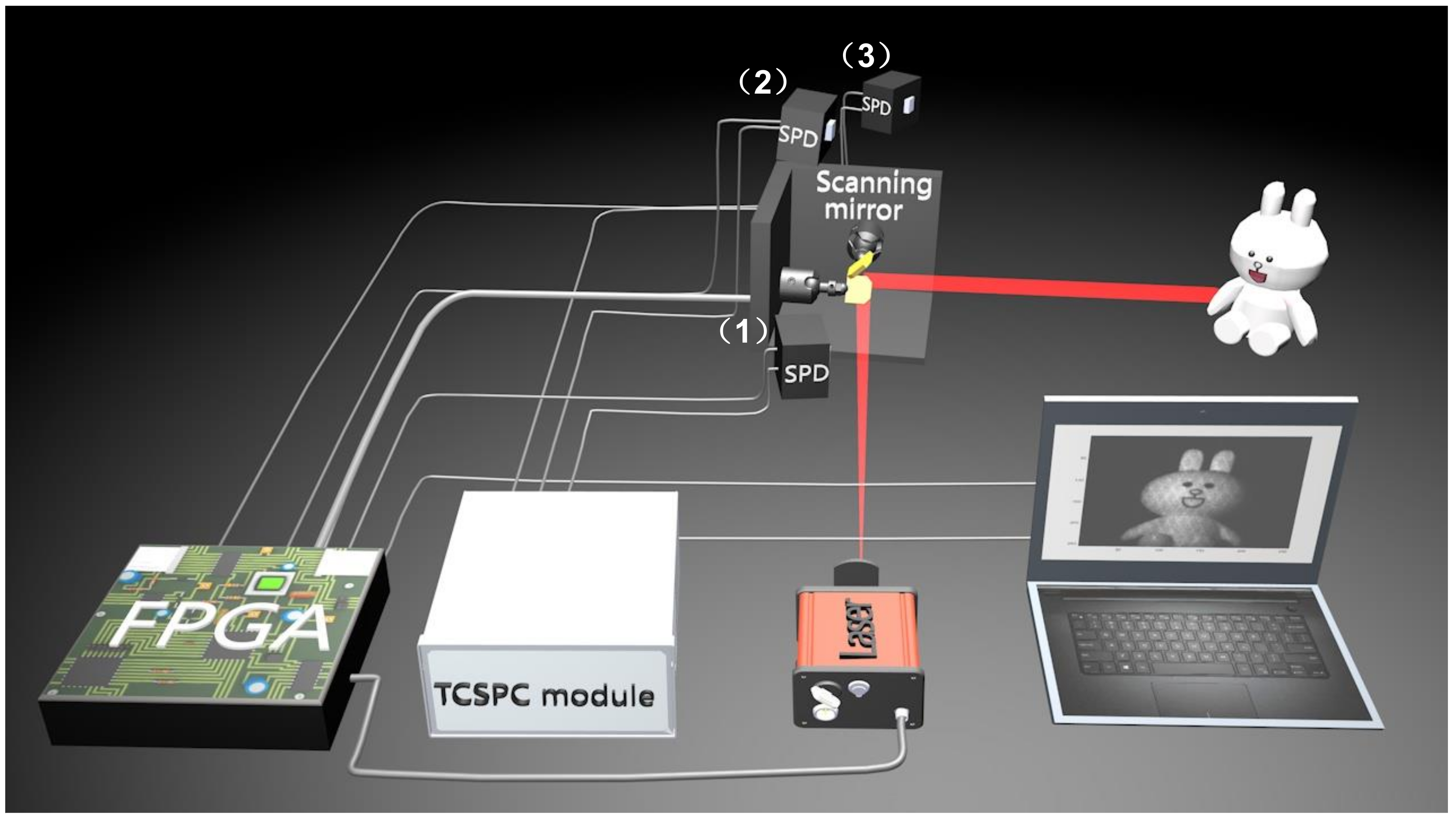
3.3. 3D Imaging Experiment Based on Photometric Stereo Algorithm

The photometric stereo algorithm is a method to reconstruct the 3D model of an object from multiple images. It uses a set of cameras to take pictures of objects from different directions and then obtains the 3D information by calculating the reflectivity and surface normal vector [37]. We define the direction of the light source is L , the normal unit vector of a point on the surface of the object is N , the reflectivity is ρ and the intensity of the pixel on the corresponding image is I. Then we can get the Lambert model
I = ρ N · L ,
where
N = N x , N y , N z T = p p 2 + q 2 + 1 , q p 2 + q 2 + 1 , 1 p 2 + q 2 + 1 T ,
T represents the matrix transpose operator, p and q respectively represent the two gradient directions on the surface of the object. Assuming that there are three known non-coplanar light directions, then Equation (11) can be obtained. Because L is a full rank matrix, the normal vector can be expressed as N = 1 ρ I · L 1 . Then we can get the depth information by integrating the normal vector of the object surface,
I 1 = ρ L 11 N x + L 12 N y + L 13 N z I 2 = ρ L 21 N x + L 22 N y + L 23 N z I 3 = ρ L 31 N x + L 32 N y + L 33 N z
Figure 7 shows the experimental setup. Three SPDs are used in this experiment to detect the 3D object (a rabbit model with a size of 4 cm × 3 cm × 7 cm ) from different directions, which need to be calibrated in advance. The experimental data is processed by the photometric stereo algorithm to obtain a 3D image of the object. As shown in Figure 8, the method can reconstruct the 3D model of the object well.

4. Conclusions

In summary, a 3D imaging scheme based on TCSPC technology has been proposed and demonstrated. In the scheme, we adopt the range-gated technology to reduce environmental noise and improve the SSIM of imaging results by 10 times. At the same time, the TOF algorithm and photometric stereo algorithm are used for three-dimensional imaging of objects. Experiments show that the proposed scheme can realize imaging with a lateral resolution of 512 × 512 and an axial resolution of 4.2 mm. Finally, the proposed imaging scheme has the potential to be widely used in imaging in complicated environments, especially in remote, haze and underwater.

Author Contributions

Conceptualization and methodology, H.Z., Y.Z. and C.F.; software, C.F. and G.W.; validation, C.F., H.Z. and H.C.; formal analysis, G.W.; investigation, Y.H.; resources, H.C.; data curation, C.F.; writing–original draft preparation, C.F.; writing–review and editing, C.F., H.Z., Y.Z. and J.L.; visualization, H.C. and J.L.; project administration and Supervision, J.S. and Z.X. All authors have read and agreed to the published version of the manuscript.

Funding

This research was supported by Shanxi Key Research and Development Project (Grant No. 2019ZDLGY09-10); Key Innovation Team of Shaanxi Province (Grant No. 2018TD-024) and 111 Project of China (Grant No.B14040).

Conflicts of Interest

The authors declare no conflict of interest.

References

  1. Chhabra, P.; Maccarone, A.; McCarthy, A.; Buller, G.; Wallace, A. Discriminating underwater lidar target signatures using sparse multi-spectral depth codes. In Proceedings of the 2016 Sensor Signal Processing for Defence (SSPD), Edinburgh, UK, 22–23 September 2016; pp. 1–5. [Google Scholar]
  2. Becker, W. Advanced Time-Correlated Single Photon Counting Techniques; Springer Series in Chemical Physics; Springer: Berlin/Heidelberg, Germany, 2005. [Google Scholar]
  3. Buller, G.S.; Collins, R.J. Single-photon generation and detection. Meas. Sci. Technol. 2010, 21, 012002. [Google Scholar] [CrossRef]
  4. Ware, W.R. Fluorescence Lifetime Measurements by Time Correlated Single Photon Counting; Technical Report; University of Minnesota: Minneapolis, MN, USA, 1969. [Google Scholar]
  5. Ware, W.R. Transient luminescence measurements. Creat. Detect. Excit. State 1971, 1, 213. [Google Scholar]
  6. Schuyler, R.; Isenberg, I. A monophoton fluorometer with energy discrimination. Rev. Sci. Instrum. 1971, 42, 813–817. [Google Scholar] [CrossRef]
  7. Bachrach, R. A photon counting apparatus for kinetic and spectral measurements. Rev. Sci. Instrum. 1972, 43, 734–737. [Google Scholar] [CrossRef]
  8. Binkert, T.; Tschanz, H.; Zinsli, P. The measurement of fluorescence decay curves with the single-photon counting method and the evaluation of rate parameters. J. Lumin. 1972, 5, 187–217. [Google Scholar] [CrossRef]
  9. Lewis, C.; Ware, W.R.; Doemeny, L.J.; Nemzek, T.L. The Measurement of Short-Lived Fluorescence Decay Using the Single Photon Counting Method. Rev. Sci. Instrum. 1973, 44, 107–114. [Google Scholar] [CrossRef]
  10. Love, L.C.; Shaver, L. Time correlated single photon technique: Fluorescence lifetime measurements. Anal. Chem. 1976, 48, 364A–371A. [Google Scholar] [CrossRef]
  11. Becker, W.; Bergmann, A.; König, K.; Tirlapur, U. Picosecond fluorescence lifetime microscopy by TCSPC imaging. In Multiphoton Microscopy in The Biomedical Sciences; International Society for Optics and Photonics: Bellingham, WA, USA, 2001; Volume 4262, pp. 414–419. [Google Scholar]
  12. Becker, W.; Bergmann, A.; Hink, M.; König, K.; Benndorf, K.; Biskup, C. Fluorescence lifetime imaging by time-correlated single-photon counting. Microsc. Res. Tech. 2004, 63, 58–66. [Google Scholar] [CrossRef]
  13. Degnan, J.J. Satellite laser ranging: Current status and future prospects. IEEE Trans. Geosci. Remote Sens. 1985, GE-23, 398–413. [Google Scholar] [CrossRef]
  14. Massa, J.S.; Wallace, A.M.; Buller, G.S.; Fancey, S.; Walker, A.C. Laser depth measurement based on time-correlated single-photon counting. Opt. Lett. 1997, 22, 543–545. [Google Scholar] [CrossRef] [Green Version]
  15. Massa, J.S.; Buller, G.S.; Walker, A.C.; Cova, S.; Umasuthan, M.; Wallace, A.M. Time-of-flight optical ranging system based on time-correlated single-photon counting. Appl. Opt. 1998, 37, 7298–7304. [Google Scholar] [CrossRef] [PubMed] [Green Version]
  16. Degnan, J.J. Photon-counting multikilohertz microlaser altimeters for airborne and spaceborne topographic measurements. J. Geodyn. 2002, 34, 503–549. [Google Scholar] [CrossRef] [Green Version]
  17. Ren, M.; Gu, X.; Liang, Y.; Kong, W.; Wu, E.; Wu, G.; Zeng, H. Laser ranging at 1550 nm with 1-GHz sine-wave gated InGaAs/InP APD single-photon detector. Opt. Express 2011, 19, 13497–13502. [Google Scholar] [CrossRef] [PubMed] [Green Version]
  18. Chen, S.; Liu, D.; Zhang, W.; You, L.; He, Y.; Zhang, W.; Yang, X.; Wu, G.; Ren, M.; Zeng, H.; et al. Time-of-flight laser ranging and imaging at 1550 nm using low-jitter superconducting nanowire single-photon detection system. Appl. Opt. 2013, 52, 3241–3245. [Google Scholar] [CrossRef] [PubMed] [Green Version]
  19. McCarthy, A.; Collins, R.J.; Krichel, N.J.; Fernández, V.; Wallace, A.M.; Buller, G.S. Long-range time-of-flight scanning sensor based on high-speed time-correlated single-photon counting. Appl. Opt. 2009, 48, 6241–6251. [Google Scholar] [CrossRef] [Green Version]
  20. McCarthy, A.; Ren, X.; Della Frera, A.; Gemmell, N.R.; Krichel, N.J.; Scarcella, C.; Ruggeri, A.; Tosi, A.; Buller, G.S. Kilometer-range depth imaging at 1550 nm wavelength using an InGaAs/InP single-photon avalanche diode detector. Opt. Express 2013, 21, 22098–22113. [Google Scholar] [CrossRef] [Green Version]
  21. Henriksson, M.; Larsson, H.; Grönwall, C.; Tolt, G. Continuously scanning time-correlated single-photon-counting single-pixel 3-D lidar. Opt. Eng. 2016, 56, 031204. [Google Scholar] [CrossRef]
  22. Gordon, K.; Hiskett, P.; Lamb, R. Advanced 3D imaging lidar concepts for long range sensing. In Advanced Photon Counting Techniques VIII; International Society for Optics and Photonics: Bellingham, WA, USA, 2014; Volume 9114, p. 91140G. [Google Scholar]
  23. Kostamovaara, J.; Huikari, J.; Hallman, L.; Nissinen, I.; Nissinen, J.; Rapakko, H.; Avrutin, E.; Ryvkin, B. On laser ranging based on high-speed/energy laser diode pulses and single-photon detection techniques. IEEE Photonics J. 2015, 7, 1–15. [Google Scholar] [CrossRef]
  24. Pawlikowska, A.M.; Halimi, A.; Lamb, R.A.; Buller, G.S. Single-photon three-dimensional imaging at up to 10 kilometers range. Opt. Express 2017, 25, 11919–11931. [Google Scholar] [CrossRef]
  25. Kang, Y.; Li, L.; Liu, D.; Li, D.; Zhang, T.; Zhao, W. Fast long-range photon counting depth imaging with sparse single-photon data. IEEE Photonics J. 2018, 10, 1–10. [Google Scholar] [CrossRef]
  26. Li, Z.; Wu, E.; Pang, C.; Du, B.; Tao, Y.; Peng, H.; Zeng, H.; Wu, G. Multi-beam single-photon-counting three-dimensional imaging lidar. Opt. Express 2017, 25, 10189–10195. [Google Scholar] [CrossRef] [PubMed]
  27. Li, Z.P.; Huang, X.; Cao, Y.; Wang, B.; Li, Y.H.; Jin, W.; Yu, C.; Zhang, J.; Zhang, Q.; Peng, C.Z.; et al. Single-photon computational 3D imaging at 45 km. arXiv 2019, arXiv:1904.10341. [Google Scholar]
  28. Kirmani, A.; Venkatraman, D.; Shin, D.; Colaço, A.; Wong, F.N.; Shapiro, J.H.; Goyal, V.K. First-photon imaging. Science 2014, 343, 58–61. [Google Scholar] [CrossRef] [PubMed]
  29. Liu, X.; Shi, J.; Wu, X.; Zeng, G. Fast first-photon ghost imaging. Sci. Rep. 2018, 8, 5012. [Google Scholar] [CrossRef]
  30. Kong, H.J.; Kim, T.H.; Jo, S.E.; Oh, M.S. Smart three-dimensional imaging ladar using two Geiger-mode avalanche photodiodes. Opt. Express 2011, 19, 19323–19329. [Google Scholar] [CrossRef]
  31. Huang, P.; He, W.; Gu, G.; Chen, Q. Depth imaging denoising of photon-counting lidar. Appl. Opt. 2019, 58, 4390–4394. [Google Scholar] [CrossRef]
  32. Wang, Z.; Bovik, A.C.; Sheikh, H.R.; Simoncelli, E.P. Image quality assessment: From error visibility to structural similarity. IEEE Trans. Image Process. 2004, 13, 600–612. [Google Scholar] [CrossRef] [Green Version]
  33. Tobin, R.; Halimi, A.; McCarthy, A.; Laurenzis, M.; Christnacher, F.; Buller, G.S. Three-dimensional single-photon imaging through obscurants. Opt. Express 2019, 27, 4590–4611. [Google Scholar] [CrossRef]
  34. Xin, S.; Nousias, S.; Kutulakos, K.N.; Sankaranarayanan, A.C.; Narasimhan, S.G.; Gkioulekas, I. A theory of fermat paths for non-line-of-sight shape reconstruction. In Proceedings of the 2019 IEEE/CVF Conference on Computer Vision and Pattern Recognition (CVPR), Long Beach, CA, USA, 15–20 June 2019; pp. 6800–6809. [Google Scholar]
  35. Li, S.; Zhang, Z.; Ma, Y.; Zeng, H.; Zhao, P.; Zhang, W. Ranging performance models based on negative-binomial (NB) distribution for photon-counting lidars. Opt. Express 2019, 27, A861–A877. [Google Scholar] [CrossRef]
  36. Snyder, D.L. Random Point Processes; Wiley: Hoboken, NJ, USA, 1975. [Google Scholar]
  37. Holroyd, M.; Lawrence, J.; Humphreys, G.; Zickler, T. A photometric approach for estimating normals and tangents. ACM Trans. Graph. (TOG) 2008, 27, 133. [Google Scholar] [CrossRef]
Figure 1. The schematic diagram of TCSPC: (a) TCSPC module records the start-stop-time between the pulse emitted by the laser and the photon detected by SPD; (b) histogram of the number of photons vs. the arrival time.
Applsci 10 01930 g001
Figure 2. The schematic of the experimental setup. FPGA controls the laser emission and the scanning mirror rotation, and sends gating signal to SPD. Scanning mirror scans the object according to the scanning mode preset by FPGA. The computer can get the image of the object by rearranging the photon signals of HydraHarp 400 according to the preset scanning mode of scanning mirror.
Applsci 10 01930 g002
Figure 3. Results of noise reduction experiment based on the range-gated technology. SP represents the number of signal photons. The left side represents the imaging result without gating, and the right side indicates the result with gating. The signal photons decrease from 3000 cps to 500 cps and the noise photons are keep at 10,000 cps.
Applsci 10 01930 g003
Figure 4. Analysis of noise reduction experiment based on range-gated technology.
Applsci 10 01930 g004
Figure 5. (a) The original object. (b) Experimental imaging result.
Applsci 10 01930 g005
Figure 6. (a) Measurement results of laser waveform. The full width half maximum (FWHM) is 90 ps. (b) Measurement results: the blue curve is the reference value measured by high precision stepper motor, and the red dots are the measured value of ten experiments. (c) The errors between the measured value and the reference value.
Applsci 10 01930 g006
Figure 7. The schematic of the experimental setup for 3D imaging based on photometric stereo algorithm. Three SPDs are used in this experiment, and the object is a rabbit model with a size of 4 cm × 3 cm × 7 cm . The distance between the detectors and the object is 35 cm.
Applsci 10 01930 g007
Figure 8. (a) The original object. (bd) are the imaging results of three SPDs detect the object from different directions. (e) 3D imaging result of the photometric stereo algorithm.
Applsci 10 01930 g008

