Highly Directive Biconic Antennas Embedded in a Dielectric

Featured Application

efficient and secure point-to-point wireless communication; radiating energy transfer systems

Abstract

Designing antennas suitable for generating highly directive electromagnetic signals has become a fundamental task. This is particularly relevant for the development of efficient and sustainable point-to-point communication channels, and for energy transfer. Indeed, these are nowadays expanding areas of research. In order to deal with said particular wave phenomena, an extension of the electrodynamics equations is taken into account, where exact solitonic type solutions are admitted. These waves may have compact support and travel along a straight line, without dissipation, at the speed of light. The result suggests the design of biconic type antennas having specific properties that are numerically examined in this paper. The cones, supplied with an oscillating source, are embedded in a dielectric material of suitable shape, with the purpose of driving the signal in the proper direction. The computations based on the extended model are aimed toward simulating the possibility of generating peculiar wave behaviors, in view of practical implementations in the framework of point-to-point communications or wireless power transmission.

1. Introduction

Highly directive electromagnetic fields involved in point-to-point (P2P) communications represent a desired aspect of information/energy transmission, in those applications where not being intercepted is important. This aspect is not only required for securing a private communication channel, but also to increase the efficiency in energy transfer, thereby limiting the release of a great amount of wasted energy in neighboring media. Typical commercial solutions involve the beaming of microwaves through parabolic reflectors, laser beams carrying encoded data and short distance Wi-Fi communication systems. Free space optical (FSO) communications are used for short distance, high bandwidth transmissions. They typically rely on coherent sources, but suffer from atmospheric fluctuations in the moisture content (particularly fog), severely affecting the link. Therefore, more promising applications of FSOs are found inside chips [1]. Radio Frequency (RF) links are preferred to secure higher bandwidths over longer distances and for extended periods of time. Nevertheless, their energy efficiency is lower in comparison to FSOs, and this aspect justifies our research.

Nowadays we may cite the ThoR consortium, active in Europe and Japan, working with state-of-the-art chip sets and modems operating in the standardized 60 and 70–80 GHz bands. Very recent applications (see [2]) allow one to build RF wireless P2P links featuring >100 Gbps over 1 km at 300 GHz. The quest for high bandwidth links has increased the center frequency, so currently radar bands [3] and millimeter waves (THz) [4] are studied as possible extensions of 5G and beyond technologies, further strengthening the importance of establishing directive links. It has to be noted that, as the energy increases with center frequency, so does the concern for impacts on human health—controversial results have been found [5]. Another aspect of relevance is wireless power transmission (WPT), fueled by the escalation of Internet-of-Things (IoT) (see [6,7]). Here, a crowd of sensor nodes dispersed in a physical environment requires either a distributed energy harvesting capability, or the wireless transmission of energy from a central harvesting unit. In WPT applications, three approaches have been developed: (i) near-field coupling of inductive or capacitive loads in resonant or non-resonant mode; (ii) far-field directive power beaming; (iii) far-field non-directive power transfer. Item (i) is used for extremely small scale environments; (ii), which is our aim, is used for intentional power transfer from nodes in a broader network and implements radio frequencies or microwave means; (iii) is used for electromagnetic energy harvesting of sources nonintentionally conceived for the scope (see, e.g., [8]). The benefits of using directional antennas instead of omni-directional ones in wireless sensor networks (WSNs) have been pointed out, e.g., in [9], in order to significantly reduce interference between network components. Several models of directional antenna in the framework of WSNs are compared in [10]. There are currently two categories of commercial directive radio antennas: On one hand are the traditional ones, including helix, log periodic array antennas, aperture horn antennas, reflectors and patch antennas. On the other hand are smart antennas, each consisting of an array of elements that can offer adaptive transmission. Depending on the specific application, shapes, sizes and designs of directional antennas can be quite different. The signal pattern from a directional antenna consists of a cigar-shaped great lobe, usually surrounded by smaller side lobes. For a survey on radiation patterns of these devices and an application on wireless networks, we mention, for instance, [11,12].

2. Motivation

Our aim was to design special antennas able to convey the electromagnetic signal along patterns characterized by extremely high directivity, ameliorated in comparison to existing commercial solutions. The basic structure we sought is that of biconic antennas, although other geometries might be taken into account. The goal was to predict the possibility of generating peculiar waves that can be employed in P2P communications or WPT applications in a much more energy efficient way. The cones, supplied with an oscillating source of the proper frequency, are embedded in a dielectric material. The shape of this medium is designed in order to drive the signal in a specified direction by respecting the classical rules of geometrical optics. Recent similar results on this subject are provided for instance in [13], although the functioning principles of those devices are rather different from the ones considered here.

3. Contributions

In [14,15], an original extension of the equations ruling electromagnetic phenomena has been introduced in order to allow for the existence of solitonic type solutions. That extension features important properties, such as the existence of a Lagrangian, the possibility to prove Lorenz’s invariance (in the case of the so called free-waves; see Section 5) and the possibility to write the equations in covariant form. Note that all the classical Maxwellian solutions are included in the new model. In addition, other waves, whose explicit expression is known in many circumstances, may exist: they display concentrated support and travel along straight paths at the speed of light. This is the most significant contribution we gave to the field of electromagnetic transmissions, enabling the analysis of new exciting phenomena. Hypothetically, a directivity factor equal to infinity could be achieved, although we think that in practice one should stay on more realistic ground. Our computations, based on finite difference techniques, actually show the ability to simulate signals having excellent directional properties. Some preliminary laboratory tests (not documented here) anticipate the project feasibility. These practical results are expected to be published in the near future.

4. An Extended Formulation for Electrodynamics

In order to fix the notation, we start by writing the set of Maxwell equations in SI unit convention:

$$\nabla ·\mathit{D}={\rho }_s$$

(1)

$$\nabla \times \mathit{H}-\frac{\partial \mathit{D}}{\partial t}={\mathit{J}}_s$$

(2)

$$\nabla \times \mathit{E}+\frac{\partial \mathit{B}}{\partial t}=0$$

(3)

$$\nabla ·\mathit{B}=0$$

(4)

where, as usual, $\mathit{D}$ is the displacement field, ${\rho }_s$ represents the charge sources in the medium, $\mathit{H}$ is the magnetic strength field, ${\mathit{J}}_s$ is the current source in the medium, $\mathit{E}$ is the electric field and $\mathit{B}$ is the magnetic induction field. In a vacuum and in the absence of field sources, the right hand sides of Equations (1) and (2) are set to zero. In many relevant cases, these equations are coupled with some constitutive relations—for instance: $\mathit{D}={\epsilon }_0\mathit{E}+\mathit{P}$ ($\mathit{P}$ being the polarization density) and $\mathit{H}=\mathit{B}/{\mu }_0-\mathit{M}$ ($\mathit{M}$ being the magnetization). As is customary, ${\epsilon }_0$ and ${\mu }_0$ denote the dielectric constant and the magnetic permeability in a vacuum, respectively. To complete the set, it is customary to add the equation expressing the Lorentz’s force on a given charge q traveling in an electromagnetic field with velocity $\mathit{v}$; i.e.,

$$\mathit{F}=q(\mathit{E}+\mathit{v}\times \mathit{B})$$

(5)

We now introduce the extensions of the equations as proposed in [14,15], wherein the possibility to have nonzero divergence ($\nabla ·\mathit{E}\ne 0$) for the electric field in a vacuum, even in the absence of sources, was postulated. This assumption produces an extra current term in the Ampère’s law. As a consequence of this revision, two new variables and two new unknowns were added to the standard system. The main motivation for this extension was the possibility to expand the set of possible solutions. The reviewed model has the advantage of incorporating solitary signal-packets with compact support (solitons) within the framework of a differential theory. The term "soliton" commonly refers to solutions of certain nonlinear equations that are initially localized in space and evolve while maintaining their shape (see, e.g., [16]). In our case, these will be smooth electromagnetic waves with compact support traveling (in the simplest situation) along a straight trajectory at the speed of light. Note that these entities are not available in the solution space of the classical Maxwell equations. In suitable circumstances, these solitons may be assimilated to “photons”, as those emanated or absorbed by matter upon proper solicitations. With this interpretation, the photon is not the “carrier” of the electromagnetic field anymore, but becomes a pure wave, carrying along electric and magnetic components. In the present paper, we do not want to stress the reader with these aspects. More insights on these issues can be found in [15].

For the time being, let us suppose we are working in a vacuum. According to [14], by letting the divergence of the electric field be different from zero, we arrive at the following formulation:

$$\frac{\partial \mathit{E}}{\partial t}=c^2\nabla \times \mathit{B}-\rho \mathit{V}$$

(6)

$$\frac{\partial \mathit{B}}{\partial t}=-\nabla \times \mathit{E}$$

(7)

$$\nabla ·\mathit{B}=0$$

(8)

$$\frac{\partial p}{\partial t}=\widehat{\mu }\rho \mathit{E}·\mathit{V}$$

(9)

$$\rho \left[\frac{D\mathit{V}}{Dt}+\widehat{\mu }\left(\mathit{E}+\mathit{V}\times \mathit{B}\right)\right]=-\nabla p$$

(10)

where, by definition, $\rho =\nabla ·\mathit{E}$ is the divergence of the electric field. This nonlinear system counts ten unknowns, namely, the three components of the electric field $\mathit{E}$, the three components of the magnetic induction $\mathit{B}$, the three components of the wave velocity field $\mathit{V}$ and the scalar function p. Basically, here we are only considering the case of a linear homogeneous medium, corresponding to $\mathit{D}={\epsilon }_0\mathit{E}$ and $\mathit{B}=\mathit{H}/{\mu }_0$, so that there is room for further extensions that for the moment are not taken into account.

The first Equation (6) is Ampère’s law where the additional term $\rho \mathit{V}$ has to be interpreted as a free flow of immaterial current with density $\rho$, associated with the evolution of an electromagnetic phenomenon. In principle, this latter term can be summed up to the classical one (not present in (6)), due to the flow of current along a conductive medium that may interact with the wave. The complete version of such a revised equation is reported in [15], Section 2. By taking in to account these additional contributions, it is possible to model the mutual interactions between wave and guides, as studied later in this paper.

Equation (10) is basically the Euler’s equation for non-viscous fluids. On the left-hand side we find the divergence of the electric field, multiplied by the sum of two terms: the first one is the total derivative ${\displaystyle \frac{D\mathit{V}}{Dt}:=\frac{\partial \mathit{V}}{\partial t}+(\mathit{V}·\nabla )\mathit{V}}$; the second one, $\mathit{E}+\mathit{V}\times \mathit{B}$, recalls the Lorentz’s law. The constant $\widehat{\mu }$ appearing in (10) has the dimension of a charge divided by a mass and has been estimated to be approximately equal to $2.85\times {10}^{11}$ Coulomb/Kg (see [15], Appendix G). On the right-hand side, there is the gradient of a potential p, which analogously to the Euler’s equation, plays the role of pressure. We may actually treat the potential p as a kind of pressure term that can assume both positive and negative values, and has dimensions equal to velocity over a time squared. Indeed, from a dimensional analysis it turns out that ${ϵ}_{0}p/\widehat{\mu }$ is a force per unity of surface. Equation (9) follows from energy conservation arguments. This suggests the possibility of inducing pressure effects as a consequence of a lack of orthogonality between $\mathit{E}$ and $\mathit{V}$ (see [17], where the model equations have been used to simulate some electromagnetic tweezer effects). It is crucial to observe that, when $\rho$, $D\mathit{V}/Dt$ and p are identically zero, one recovers the usual Maxwell Equations (1)–(4) in a vacuum. Therefore, the revised model is actually an extension of the classical one.

Equations of the type of (10), coupled with Maxwell’s ones, are usually found in some plasma physics models—for instance, those related to magnetohydrodynamics (see, for instance, [18] or [19]). In such examples, a number of charged particles evolve as a real fluid. In this fashion, $\mathit{V}$ takes the meaning of a fluid flow velocity and p is a proper pressure. Moreover, a mass density ${\rho }_m$ and a charge density ${\rho }_q$ appear in the equations. In the present model, massive charged particles are not necessarily involved. As a consequence, $\mathit{V}$, p and $\rho$ assume different meanings.

As in the case of Maxwell’s equations, by multiplying the first two equations by $\mathit{E}$ and $\mathit{B}$ respectively, and summing up, we get an energy balance relation:

$$\frac{1}{2}\frac{\partial }{\partial t}\left({\left|\mathit{E}\right|}^2+c^2{\left|\mathit{B}\right|}^2+\frac{2}{\widehat{\mu }}p\right)=-c^2\nabla ·\left(\mathit{E}\times \mathit{B}\right)$$

(11)

Finally, by taking the divergence of Equation (6), one finds the continuity equation:

$$\frac{\partial \rho }{\partial t}=-\nabla ·\left(\rho \mathit{V}\right)$$

(12)

which appears as an automatic consequence of the model equations.

In view of operating in cylindrical coordinates, we propose a suitable simplification based on symmetry arguments. This reduces the starting problem from three to two dimensions. We use the referring system $(r,\phi ,z)$, where the corresponding functions do not depend on $\phi$. We set $\mathit{E}=(E_r,0,E_z)$, $\mathit{B}=(0,B_{\phi },0)$ and $\mathit{V}=(V_r,0,V_z)$. In this way, the divergence operator in cylindrical coordinates, applied to the electric field, takes the form:

$$\rho =\frac{1}{r}\frac{\partial \left(r{E}_r\right)}{\partial r}+\frac{\partial E_z}{\partial z}$$

(13)

The other meaningful equations are:

$$\frac{\partial E_r}{\partial t}=-c^2\frac{\partial B_{\phi }}{\partial z}-\rho V_r$$

(14)

$$\frac{\partial E_z}{\partial t}=\frac{c^2}{r}\frac{\partial \left(r{B}_{\phi }\right)}{\partial r}-\rho V_z$$

(15)

$$\frac{\partial B_{\phi }}{\partial t}=-\frac{\partial E_r}{\partial z}+\frac{\partial E_z}{\partial r}$$

(16)

$$\frac{\partial p}{\partial t}=\widehat{\mu }\rho \left(E_r{V}_r+E_z{V}_z\right)$$

(17)

$$\rho \left[\frac{\partial V_r}{\partial t}+V_r\frac{\partial V_r}{\partial r}+V_z\frac{\partial V_r}{\partial z}+\widehat{\mu }\left(E_r-V_z{B}_{\phi }\right)\right]=-\frac{\partial p}{\partial r}$$

(18)

$$\rho \left[\frac{\partial V_z}{\partial t}+V_r\frac{\partial V_z}{\partial r}+V_z\frac{\partial V_z}{\partial z}+\widehat{\mu }\left(E_z+V_r{B}_{\phi }\right)\right]=-\frac{\partial p}{\partial z}$$

(19)

5. Free-Waves

An interesting subset of solutions is obtained when $D\mathit{V}/Dt$ and p are vanishing, though $\rho$ will be allowed to remain different from zero. These will be called free-waves, and in general they have the property that the triplet $(\mathit{V},\mathit{E},\mathit{B})$ is orthogonal with the additional conditions $\left|\mathit{E}\right|=\left|c\mathit{B}\right|$ and $\left|\mathit{V}\right|=c$. In this case, Equation (10) reduces to:

$$\rho \left(\mathit{E}+\mathit{V}\times \mathit{B}\right)=0$$

(20)

from which one could easily deduce the orthogonality of the couple $\mathit{E}$ and $\mathit{B}$, and that of the couple $\mathit{E}$ and $\mathit{V}$. As it is shown in Chapter 2 in [14], the reduced system of equations is invariant under Lorentz’s transformations and contains several interesting solutions not available in the Maxwellian context. We are going to introduce those that are more relevant in this discussion.

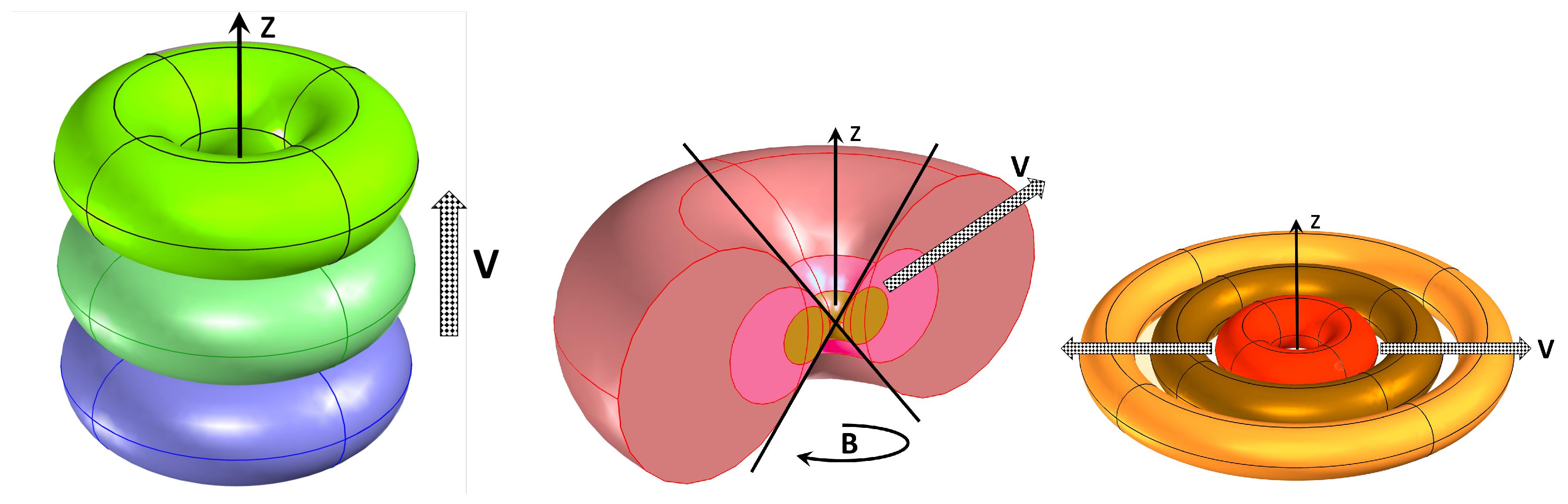
In the three dimensional cylindrical coordinate system ($r,\phi ,z$), we set:

$$\mathit{E}=(E_r,0,E_z)=\left(g\left(r\right)f(ct-z),0,0\right)$$

$$\mathit{B}=(0,B_{\phi },0)=\left(0,g\left(r\right)f(ct-z),0\right)\mathit{V}=(V_r,0,V_z)=(0,0,c)$$

(21)

Here g and f are arbitrary functions (g is only required to tend to zero as r goes to zero). Waves of this kind solve the whole set of Equations (6)–(10). The solution travels in the direction of the z-axis at speed c (see Figure 1, left). By choosing both f and g with compact support, we are able to describe solitonic solutions similar in their behavior to “photons” of any size. Some plane waves of infinite extension trivially belong to this typology. The expressions in (21) are at the foundation of the research carried out in this paper. As a matter of fact, the device proposed in Section 9 is finalized to generate this type of signal, starting from the assumption that the revised model actually predicts the possibility of such focused compact waves.

A more general situation (see again Figure 1) is obtained by defining, for a given angle $\alpha$:

$$(V_r,0,V_z)=\left(\frac{cr}{R}cos\alpha ,0,\frac{cz}{R}sin\alpha \right)$$

(22)

where $R=\sqrt{{(rcos\alpha )}^2+{(zsin\alpha )}^2}$. The choice $\alpha =\pi /2$, corresponds to the case examined above. In particular, later we will be interested in the case where $\alpha =\pi /4$. Here below, we just mention the case $\alpha =0$, where the three Equations (14)–(16) reduce to:

$$0=-c^2\frac{\partial B_{\phi }}{\partial z}-c\frac{\partial E_z}{\partial z}\frac{\partial E_z}{\partial t}=\frac{c^2}{r}\frac{\partial \left(r{B}_{\phi }\right)}{\partial r}\frac{\partial B_{\phi }}{\partial t}=\frac{\partial E_z}{\partial r}$$

(23)

One of the advantages of the extended model is the possibility of handling situations where $E_z$ and $B_{\phi }$ actually depend on z (on the contrary, the first equation in (23) would be trivially satisfied). Nevertheless, even by neglecting the dependence on z, the construction of exact solutions is rather complicated. The problem has been approached by various authors. In [20,21], efforts were made to come out with families of solutions that are successively generalized in view of applications involving waves in nonlinear media. The expressions found are nonlinear and couple the unknowns $E_z$ and $B_{\phi }$ in such a way that each one is a function of the other. Alternatively, expansions in terms of Bessel’s functions are available. The consequence of those studies is that the setting proposed in (22) is just a simplification. Indeed, we guess that $\mathit{V}$ itself nonlinearly evolves in time depending on the behavior of the electromagnetic fields. We did not pursue this analysis further. We instead performed some numerical computations based on (22), since we believed that such a setting would not alter significantly our outcomes, at least if we were suitably far away from $r=0$.

We end this section by providing some exact solutions in the spherical context. Thus, we work with a spherical system of coordinates $(R,\vartheta ,\phi )$. An electromagnetic wave displaying perfect axial-symmetric spherical fronts can be expressed by the following triplet:

$$\mathit{E}=\left(0,\frac{c}{R}g\left(\vartheta \right)f(ct-R),0\right)\mathit{V}=\left(c,0,0\right)$$

$$\mathit{B}=\left(0,0,\frac{1}{R}g\left(\vartheta \right)f(ct-R)\right)$$

(24)

where f and g are arbitrary smooth functions. These are genuine free waves, according to our definition. Note that the electric and magnetic fields have no component along the radial direction. Moreover: $\mathit{E}·\mathit{B}=0$. Since g does not depend on $\phi$, the behavior is similar to that generated by an infinitesimal oscillating dipole lined up with the z-axis. This family of solutions moves along the radial direction with velocity c, and they are modulated by the function f. The wave-fronts are the surfaces of spheres centered at the origin. By explicitly computing the divergence of the electric field, we get:

$$\nabla ·\mathit{E}=\frac{c}{R^{2}sin\vartheta }\frac{\partial \left(gsin\vartheta \right)}{\partial \vartheta }f(ct-R)$$

(25)

It turns out that there are no possibilities to impose the free divergence condition required from Equation (1) in a vacuum, unless one chooses a g value proportional to $1/sin\vartheta$ (which implies the existence of singularities at the poles). Therefore, waves with spherical fronts cannot be of Maxwellian type. Note that the well-known spherical Hertz’s solution for an infinitesimal dipole solves the entire set of Maxwell’s equations, including $\nabla ·\mathit{E}=0$. Nevertheless, its wave-fronts (i.e., the surfaces enveloping the electromagnetic field) are not spherical and $\mathit{E}$ is not orthogonal to the propagation direction. More comments on this delicate subject are provided in Appendix D in [15].

Let us also observe that the field $\mathit{V}$ in (24) has a nonvanishing divergence; i.e., $\nabla ·\mathit{V}=2c{R}^{-1}$. Note that this is also true for the field in (22). This aspect reveals that the model equation are not directly related to classical fluid dynamics, where the condition $\nabla ·\mathit{V}=0$ implies conservation of mass. No masses are involved in our case—instead, purely electromagnetic propagation in a vacuum. We are assuming however that there may be regions where $\nabla ·\mathit{E}$ is different from zero.

We can further observe that, for R tending to infinity, $\nabla ·\mathit{E}$ decreases faster than $\mathit{E}$. This shows that the non-linearity of the equations becomes weaker as the fields are evaluated far from the source. Note that the superposition principle does not hold. Nevertheless, it may be recovered for sufficiently large values of R. This agrees with the fact that the superposition principle is true in many applications involving wave propagation—for instance, in constructive and destructive interference.

6. Numerical Methods

This section is devoted to brief descriptions of the numerical methods used to approximate the system (14)–(19). Other techniques for similar problems were employed in [17,22]. Preliminary computations based on this specific cylindrical setting were tried in [23]. Our approach sticks to the framework of low-order finite difference schemes. More accurate numerical methods may be applied in future developments. For the reasons we are going to describe, we soon discarded the idea of applying the popular Yee scheme (see, e.g., [24,25]).

Consider the two Maxwell equations $\partial \mathit{E}/\partial t=c^2\nabla \times \mathit{B}$ and $\partial \mathit{B}/\partial t=-\nabla \times \mathit{E}$ relative to a region of the void space in absence of sources of any kind. Let us place ourselves in a Cartesian reference frame $(x,y,z)$. Yee’s algorithm does not explicitly implement the equations $\nabla ·\mathit{E}=0$ and $\nabla ·\mathit{B}=0$. Indeed, the space grids are structured in such a way to reproduce only the action of the curl operator. As a consequence of this choice, the divergence-free conditions are implicitly satisfied.

In a simplified context, we may assume that the fields are of the form $\mathit{E}=(E_x,E_y,0)$, $\mathit{B}=(0,0,B_z)$ and do not depend on the variable z. The scheme uses a system of two staggered grids of step h. The fields are approximated on such grids, in order to ensure that every $\mathit{E}$ component is surrounded by four $\mathit{B}$ components, and vice versa. Time discretization is performed by fractional steps, by alternating the evaluation of $\mathit{E}$ and $\mathit{B}$. In Cartesian coordinates with grid points $(x_i,y_j)$, the procedure reads as follows:

$${\left(B_z\right)}_{i-\frac{1}{2},j+\frac{1}{2}}^{k+\frac{1}{2}}={\left(B_z\right)}_{i-\frac{1}{2},j+\frac{1}{2}}^{k-\frac{1}{2}}+\frac{\Delta t}{h}\left({\left(E_x\right)}_{i-\frac{1}{2},j+1}^k-{\left(E_x\right)}_{i-\frac{1}{2},j}^k-{\left(E_y\right)}_{i,j+\frac{1}{2}}^k+{\left(E_y\right)}_{i-1,j+\frac{1}{2}}^k\right)$$

$${\left(E_x\right)}_{i-\frac{1}{2},j}^k={\left(E_x\right)}_{i-\frac{1}{2},j}^{k-1}+\frac{c^2\Delta t}{h}\left({\left(B_z\right)}_{i-\frac{1}{2},j+\frac{1}{2}}^{k-\frac{1}{2}}-{\left(B_z\right)}_{i-\frac{1}{2},j-\frac{1}{2}}^{k-\frac{1}{2}}\right)$$

$${\left(E_y\right)}_{i,j+\frac{1}{2}}^k={\left(E_y\right)}_{i,j+\frac{1}{2}}^{k-1}-\frac{c^2\Delta t}{h}\left({\left(B_z\right)}_{i+\frac{1}{2},j+\frac{1}{2}}^{k-\frac{1}{2}}-{\left(B_z\right)}_{i-\frac{1}{2},j+\frac{1}{2}}^{k-\frac{1}{2}}\right)$$

(26)

where the index k refers to time. The numerical divergence of the electric field is calculated as follows:

$${\rho }_{i,j}^k=\frac{1}{h}\left({\left(E_x\right)}_{i+\frac{1}{2},j}^k-{\left(E_x\right)}_{i-\frac{1}{2},j}^k+{\left(E_y\right)}_{i,j+\frac{1}{2}}^k-{\left(E_y\right)}_{i,j-\frac{1}{2}}^k\right).$$

(27)

It is easy to check that ${\rho }_{i,j}^k={\rho }_{i,j}^{k-1}$, for any $k\ge 1$, which means that such a quantity is preserved during the time iterations. Many approximation schemes for the electrodynamics equations trust the fact that the divergences will not be modified during the evolution. Unfortunately, this may be true only for isolated regions of space. When any wave interacts with other objects, for example, incompatibilities grow by putting together the evolution equations, the divergence-free conditions and the boundary constraints. This fact has been made evident in [26,27], where it is shown that these restrictions are too many, so that they cannot hold together at the same time. By allowing $\nabla ·\mathit{E}$ to be different from zero we can come out from this dead end, thereby justifying the adoption of the consistent model we are examining in this paper. At this point, it should be clear that Yee’s scheme and similar ones are not appropriate for our study.

We then adopt a classical explicit (first-order) Euler method for advancing in time. The space derivatives in (14)–(16) are approximated by centered (second-order) differences. In cylindrical coordinates, we end up with the scheme at the grid point $(r_i,z_j)$:

$${\left(B_{\phi }\right)}_{i,j}^{k+1}={\left(B_{\phi }\right)}_{i,j}^k+\frac{\Delta t}{2h}\left(-{\left(E_r\right)}_{i,j+1}^k+{\left(E_r\right)}_{i,j-1}^k+{\left(E_z\right)}_{i+1,j}^k-{\left(E_z\right)}_{i-1,j}^k\right)$$

$${\left(E_r\right)}_{i,j}^{k+1}={\left(E_r\right)}_{i,j}^k+\frac{c^2\Delta t}{2h}\left({-\left(B_{\phi }\right)}_{i,j+1}^k+{\left(B_{\phi }\right)}_{i,j-1}^k\right)-\Delta t{\rho }_{i,j}^k{V}_r$$

$${\left(E_z\right)}_{i,j}^{k+1}={\left(E_z\right)}_{i,j}^k+\frac{c^2\Delta t}{2h}\left({\left(B_{\phi }\right)}_{i+1,j}^k-{\left(B_{\phi }\right)}_{i-1,j}^k\right)+\frac{c^2\Delta t}{r_i}{\left(B_{\phi }\right)}_{i,j}^k-\Delta t{\rho }_{i,j}^k{V}_z$$

(28)

For the computation of the divergence of the electric field, we used the following approximation of (13), valid in cylindrical coordinates:

$${\rho }_{i,j}^k=\frac{{\left(E_r\right)}_{i,j}^k}{r_i}+\frac{{\left(E_r\right)}_{i+1,j}^k-{\left(E_r\right)}_{i-1,j}^k}{2h}+\frac{{\left(E_z\right)}_{i,j+1}^k-{\left(E_z\right)}_{i,j-1}^k}{2h}$$

(29)

To ensure stability we must require a Courant–Friedrichs–Lewy (CFL) type condition—i.e., that the time-step $\Delta t$ is proportional to the space discretization parameter h. Such a condition is not particularly restrictive for our purposes.

Equations (9) and (10) contain the time derivatives $\partial p/\partial t$, $\partial \mathit{V}/\partial t$. It is quite simple to come out with appropriate numerical schemes for their discretization. However, in this paper we are mainly concerned with the case of free-waves (see Section 5), so that p and the total derivative $D\mathit{V}/Dt$ will be set to zero at any time. Since, in practice, $\mathit{E}$ and $\mathit{V}$ will stay orthogonal, Equation (9) becomes trivial, whereas (10) is substituted by (20). In the particular setting we are interested in, the vectors of the triplet $(\mathit{E},\mathit{B},\mathit{V})$ will constitute an orthogonal frame and satisfy $\left|\mathit{E}\right|=\left|c\mathit{B}\right|$ and $\left|\mathit{V}\right|=c$. What we just wrote is always true with the exception of some transition regions that will be described later on.

Let us notice that the approximation of (10) in its general form is far from being trivial. First of all, there is no viscous term, a property that makes the theoretical analysis and the numerical implementation quite hard. Secondly, as already pointed out in the examples of Section 5, we also have $\nabla ·\mathit{V}\ne 0$. This means that many numerical schemes available for the discretization of the equations of fluid dynamics may turn out to be unsuitable. Finally, we observe that there may be points in the computational domain where $\rho =\nabla ·\mathit{E}$ is zero (or relatively small). This is usually true in correspondence with points where $\nabla p$ is also zero. As a consequence, the unreliability of the ratio $\nabla p/\rho$ may give origins to severe instability problems in the treatment of (10). As mentioned above, here we will stay away from these situations; nevertheless, such problems exist and should be appropriately pondered within the general context.

Later in this paper, we will study the transmission of an electromagnetic wave across the interface separating media displaying different conductive properties. We describe what happens inside each medium with the help of the equations relative to free-waves. In the instant of transition, the wave is not of free type, so that suitable corrections on $\mathit{V}$ are taken into account. For simplicity, we will continue however to neglect the role of the potential p.

7. Design of the Directional Antenna

The geometry we are willing to test is shown in Figure 2. The antenna device is constituted by two conductive cones separated by a little gap. These are supplied by an alternating current via a coaxial cable (not shown in figure), carrying a frequency whose wave-length, in most applications, is of the order of the magnitude of the conductive support size. Each cone features an angle of $\pi /2$ at the vertex. The need for a gap, possibly very small, between the cones is dictated by the size of the wire connecting to the electrical source. We presume that a gap of approximately 5% of the entire size should not produce significant negative effects, but, of course, this also depends on the degree of directivity we would like to achieve.

We consider here the case where the entire antenna is immersed in a region occupied by a linear homogeneous medium $\Omega$, having phase velocity of the electromagnetic radiation lower than the speed of light in vacuum. Such a medium is characterized by a permittivity coefficient ${\epsilon }_r{\epsilon }_0>{\epsilon }_0$ and features non-magnetic properties, so that the magnetic permeability coefficient will remain ${\mu }_0$. In Figure 2, the shape is designed depending on some refraction properties that we are going to describe here below.

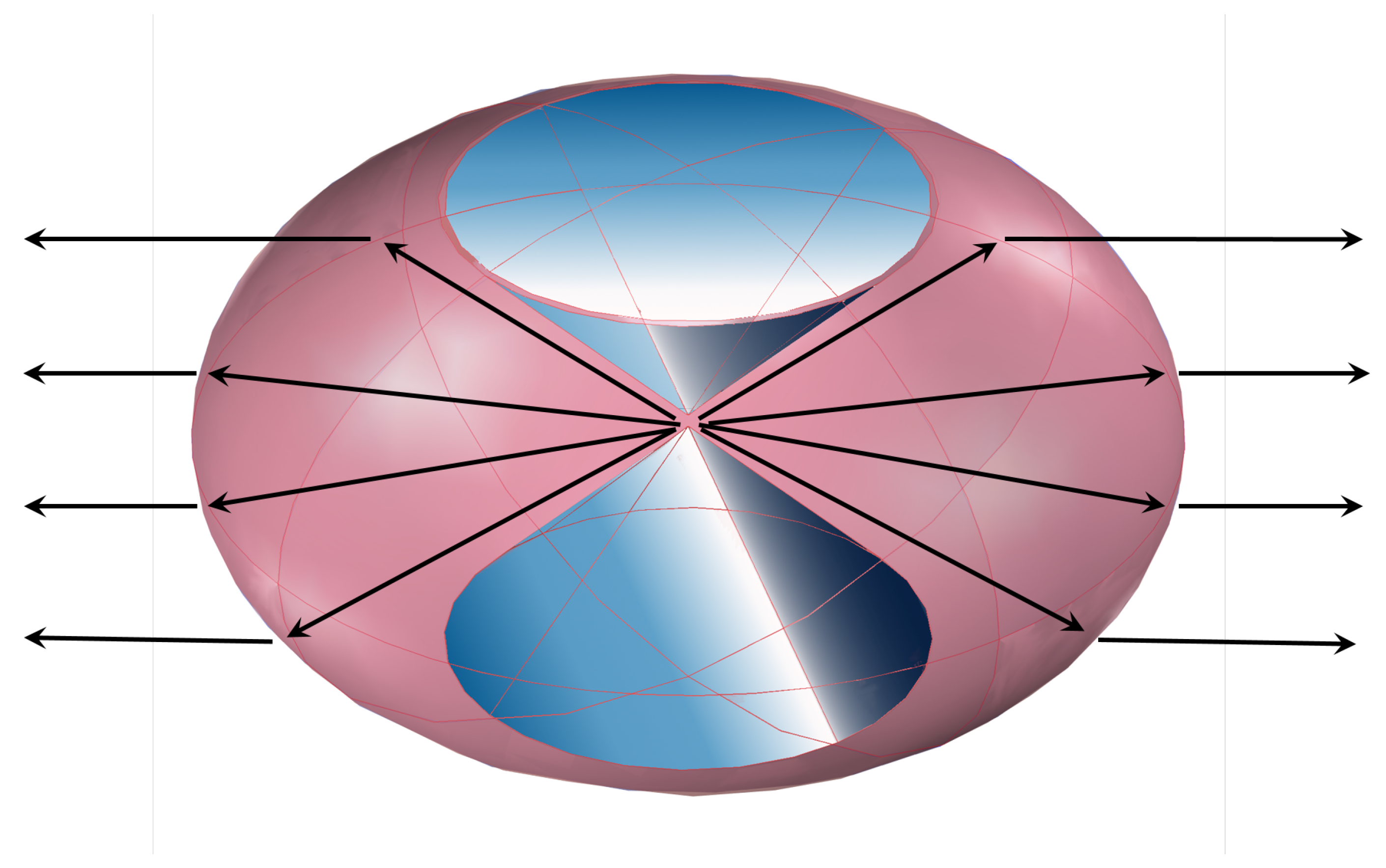
Our aim is to have a signal emerging from the antenna perfectly horizontally. In this way, the electromagnetic field follows the behavior of Figure 1 (central picture), while it remains in $\Omega$. After the transition to the outside medium (vacuum or air, in this case), the message follows instead the behavior of the right-hand side picture of Figure 1. In terms of the velocity vector $\mathit{V}$, we have the following situation. Inside $\Omega$, the magnitude of $\mathit{V}$ is: $\left|\mathit{V}\right|=1/\sqrt{{\epsilon }_r{\epsilon }_0{\mu }_0}=c/\sqrt{{\epsilon }_r}$. In the open space, we have as usual: $\left|\mathit{V}\right|=c$. At the interface between the two media, we enforce the rules of geometrical optics. We denote by $\partial \Omega$ the border of $\Omega$, i.e., the interface between the dielectric and the outside vacuum. The determination of the surface $\partial \Omega$ follows from the solution of a differential problem as explained hereafter.

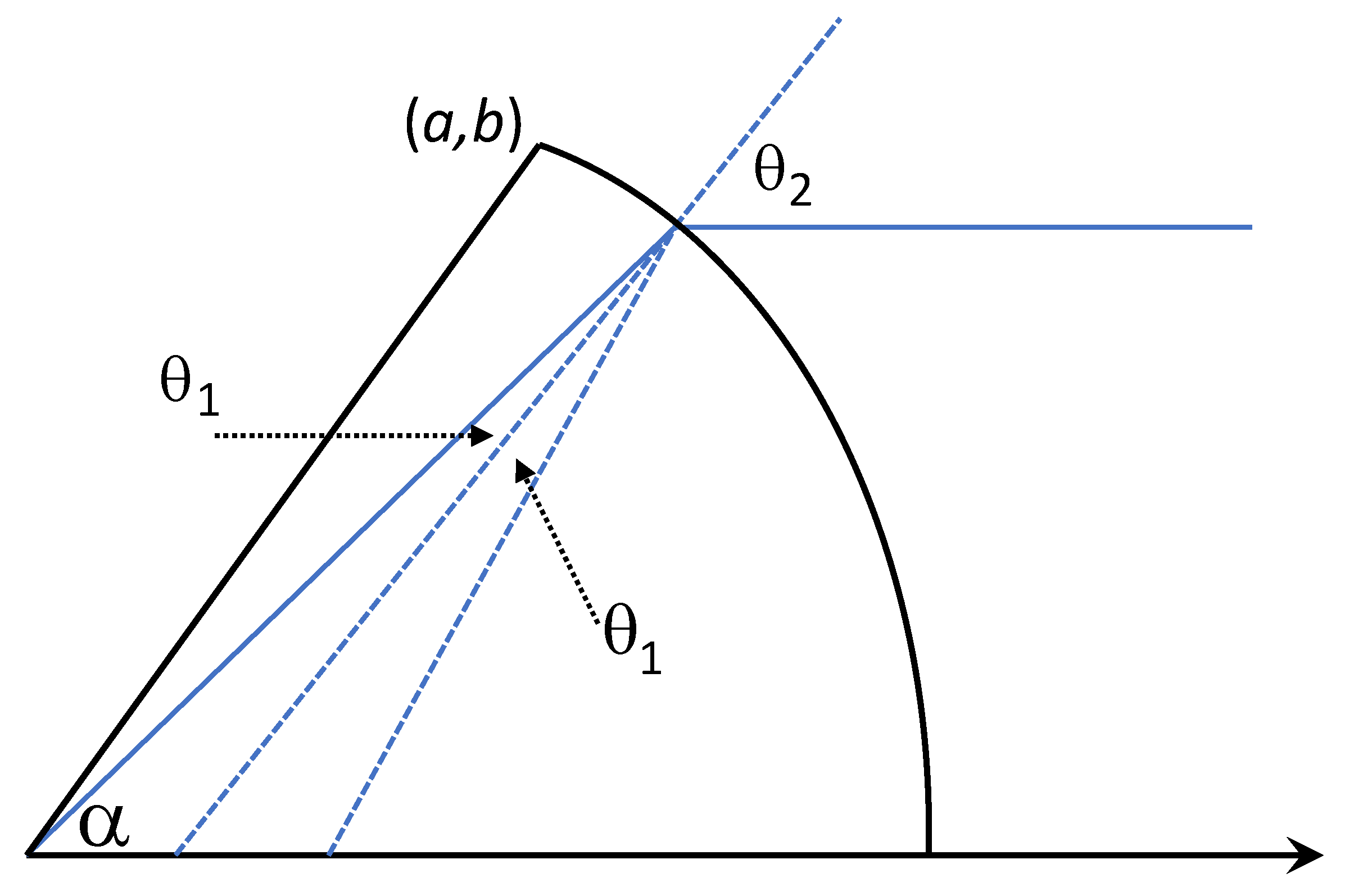
As shown in Figure 3, in the Cartesian framework $(r,z)$, $\partial \Omega$ corresponds to the graph of a function $z=s\left(r\right)$ defined through the following constraints. First of all, the curve passes through the point $(a,b)$. We have $a=b$ when the cones have the vertex angle equal to $\pi /2$ (here we are neglecting the gap between the cones). A light ray comes from the origin with an angle $\alpha$. As we said, the curve s must be designed in such a way that the emerging ray is horizontal. To proceed with the determination of s we need to recall Snell’s law (see [28], p. 38). In Figure 3, ${\vartheta }_1$ denotes the difference between $\alpha$ and the angle determined by the direction normal to $\partial \Omega$. Similarly, ${\vartheta }_2$ denotes the angle between the normal direction and the abscissa. In this particular situation, Snell’s law says that:

$$\sqrt{{\epsilon }_r}sin{\vartheta }_1=sin{\vartheta }_2$$

(30)

We can translate in formulas the above settings by writing:

$$tan\left({\vartheta }_2\right)=-\frac{1}{s^{\prime }\left(r\right)}tan\left(\alpha \right)=\frac{s\left(r\right)}{r}tan\left({\vartheta }_1\right)=tan({\vartheta }_2-\alpha )=\frac{r+s\left(r\right)s^{\prime }\left(r\right)}{s\left(r\right)-r{s}^{\prime }\left(r\right)}$$

(31)

where the prime denotes the derivative with respect to the variable r. Using the trigonometric identity $sin\vartheta =tan\vartheta /\sqrt{1+{tan}^2\vartheta }$, we get:

$$\sqrt{\frac{1}{{\epsilon }_r}}=\frac{tan\left({\vartheta }_1\right)}{tan\left({\vartheta }_2\right)}\sqrt{\frac{1+{tan}^2\left({\vartheta }_2\right)}{1+{tan}^2\left({\vartheta }_1\right)}}=\frac{r+s\left(r\right)s^{\prime }\left(r\right)}{\sqrt{r^2+s^2\left(r\right)}}.$$

(32)

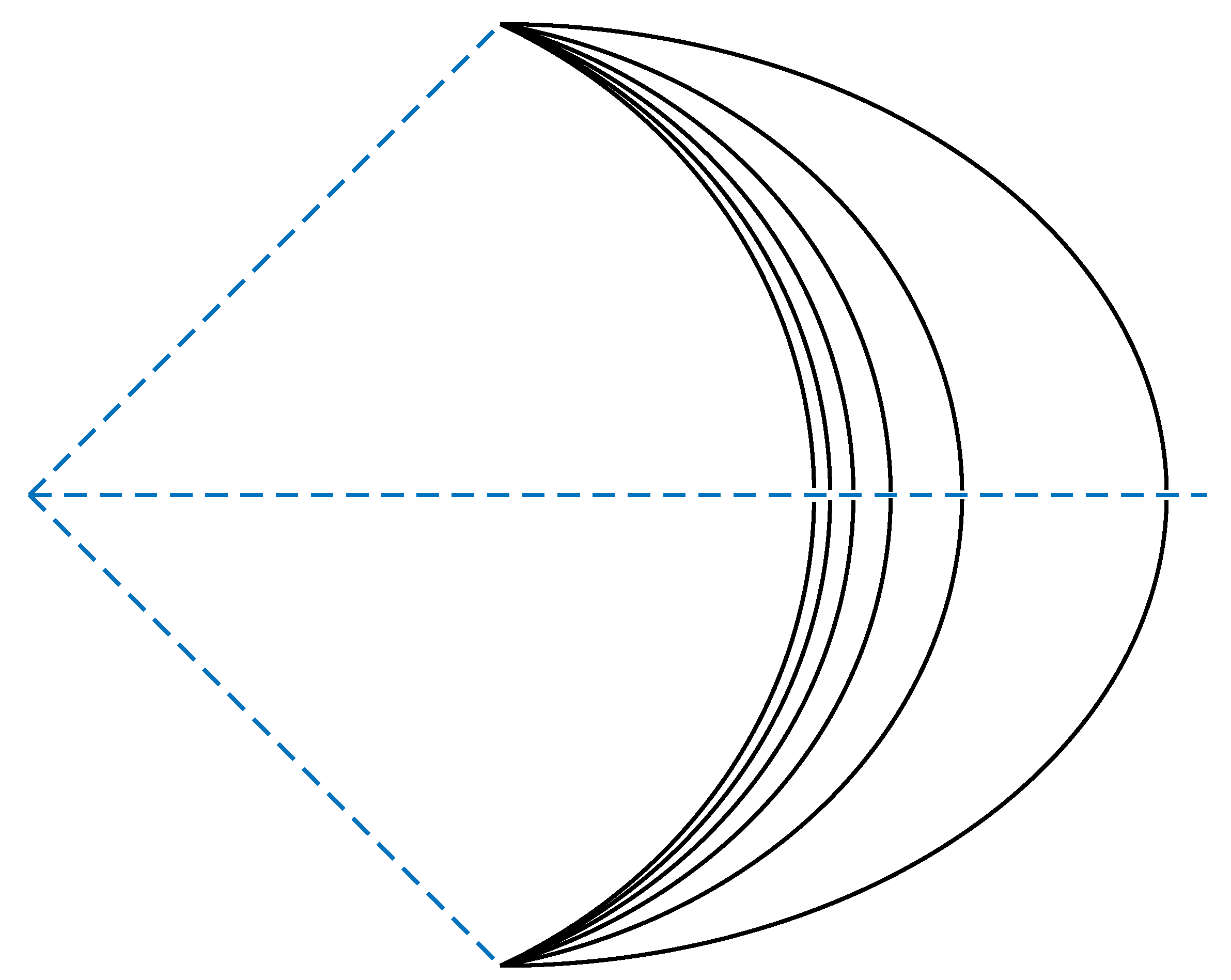
By recovering $s^{\prime }$ we finally arrive at the nonlinear differential problem:

$$\left\{\begin{array}{c}{\displaystyle s^{\prime }\left(r\right)=-\frac{1}{s\left(r\right)}\left(-r+\sqrt{\frac{r^2+s^2\left(r\right)}{{\epsilon }_r}}\right)}\hfill \\ \\ s\left(a\right)=b\hfill \end{array}\right.$$

(33)

The above differential equation may be easily solved numerically, thereby obtaining, for different values of the parameter ${\epsilon }_r$, the curves of Figure 4. One has just to pay attention to the fact that the derivative of s at the intersection with the r-axis is equal to infinity.

8. Numerical Simulations

This section is dedicated to the presentation of some numerical simulations, obtained by applying the schemes described in Section 6. The computational domain is the square $Q=[0,2L]\times [-L,L]$, where $L>0$ is a parameter. We chose by default $L=1$. The first variable is related to r and the second one to z, so that we are actually operating on a cylinder with a vertical axis. In Q, we consider a squared grid, spaced by $h:=1/N$, where N is an integer. The total number of nodes is then proportional to $N^2$. The speed of light in a vacuum is normalized to 1. The development of the process is studied in the time interval $[0,T]$, for a certain $T>0$. In order to guarantee stability, the time-step $\Delta t$ will be chosen to be suitably small.

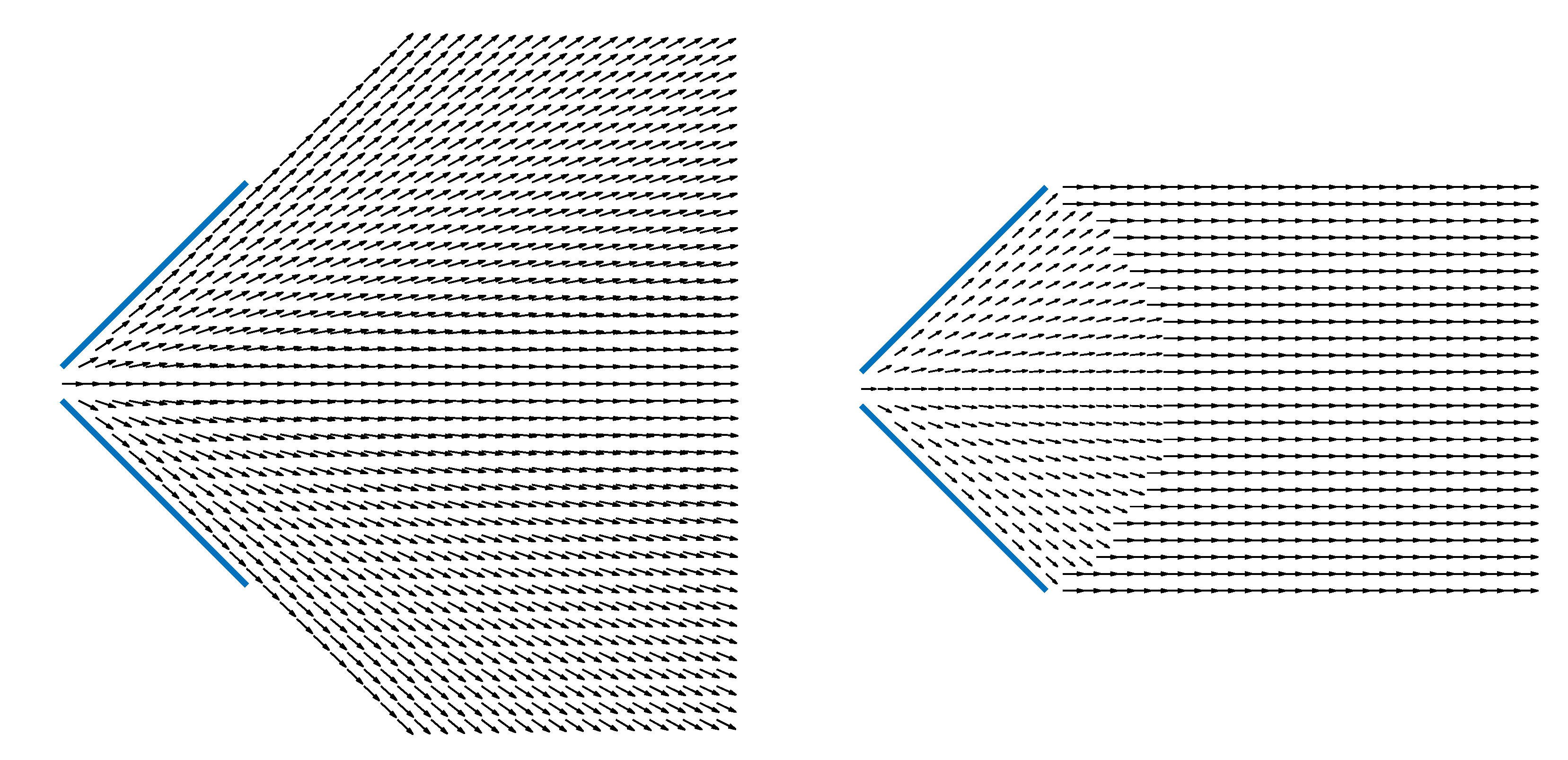
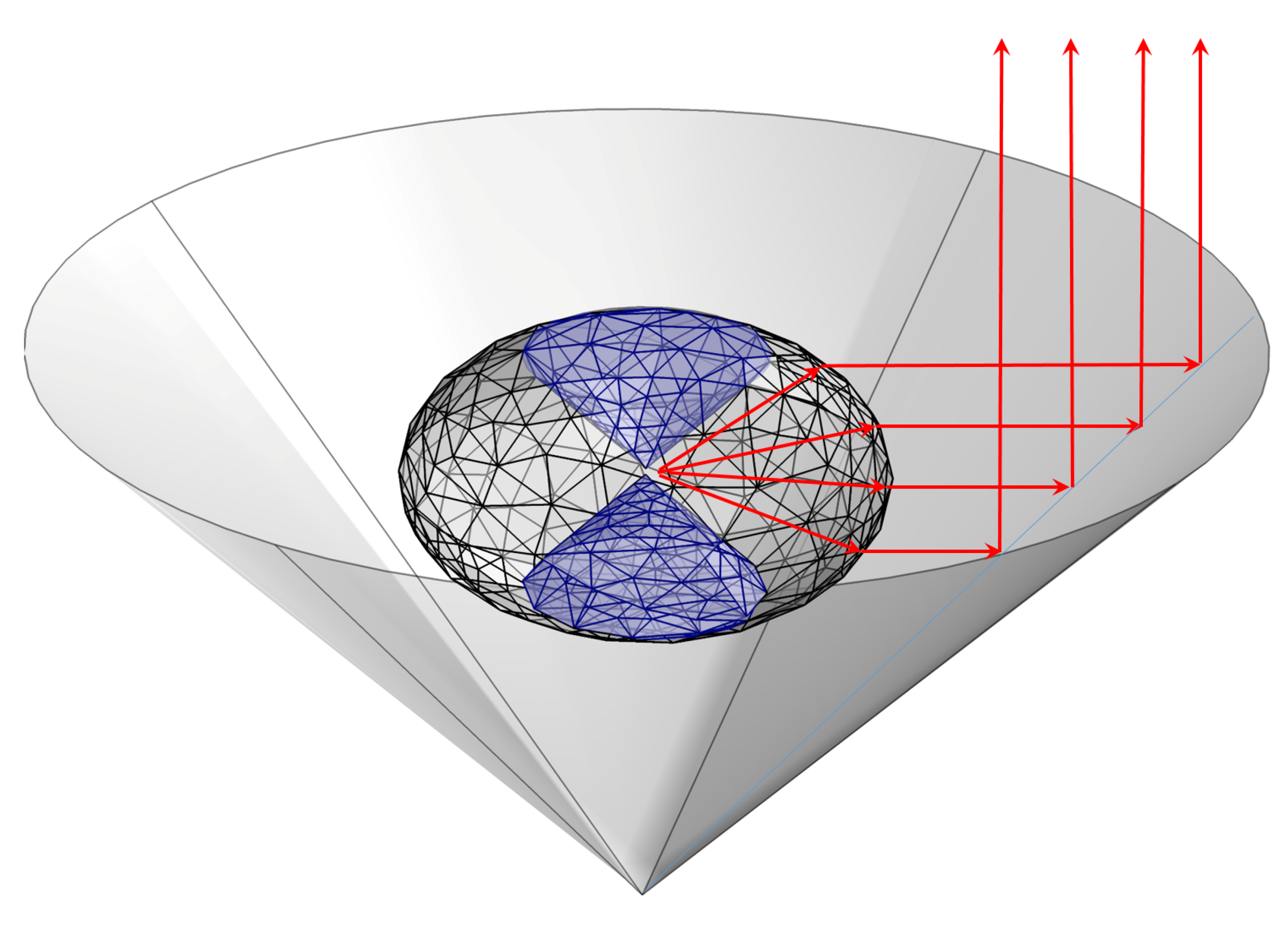
We set up in advance the velocity field $\mathit{V}$ in order to have $\left|\mathit{V}\right|=1/\sqrt{{\epsilon }_r}<1$ inside the dielectric, where we suppose that the vectors are emanating from the origin. We have $\left|\mathit{V}\right|=1$ on the remaining part of the domain where the vectors are horizontal (perpendicular to the z-axis). The deployment of the velocity field is displayed in Figure 5, for the cases when the dielectric is missing (left) and when it is present (right). In a more rigorous framework, $\left|\mathit{V}\right|$ should not be fixed in advance, but computed as time evolves according to Equations (18) and (19). As we specified in Section 6, this approach is not easily implementable from the numerical viewpoint, especially when the time advancing procedure is the trivial Euler method. Numerical solutions, in this circumstance, are too much affected by viscosity, so that the results are not reliable. Since the development of more sophisticated techniques is outside of the goals of this paper, we do not insist further on these generalizations. For the above reasons, we decided to assume that $\left|\mathit{V}\right|$ is known a priori.

As we are interested in the evolution within the region determined by the two cones of the antenna, suitable constraints are placed in the computational domain. For simplicity, we assume that these guides are perfect conductors, though the situation might be not realistic. Additionally, we should distinguish between the nodes inside the dielectric and those outside. In the transition between the two media the fields are updated by enforcing that $\mathit{B}$ remains continuous, whereas $\mathit{E}$ has a jump (these are consequences of the Fresnel’s conditions; see, e.g., [28], p. 40). In practice, we truncate to zero the longitudinal component $E_r$ at the first node just outside the dielectric.

As an initial guess, we take a portion of spherical wave. Based on (24), we set $g\left(\vartheta \right)={(sin\vartheta )}^2$ for $\pi /4\le \vartheta \le 3\pi /4$. This modulates the displacement along the transverse direction. Concerning the longitudinal direction, we take $f\left(R\right)={(cos\omega R)}^2$ with $\omega =7$ and $\pi /2\omega \le R\le 3\pi /2\omega$. The resulting electric field is shown in Figure 6 (left). The corresponding shapes of $\left|\mathit{E}\right|$ can be seen in the very first plot of Figure 7 and Figure 8. Note that this displacement has non-zero divergence ($\rho \ne 0$). The corresponding initial magnetic field is orthogonal to the plane of the figure and we have $\left|\mathit{B}\right|=\left|\mathit{E}\right|$. Successively, the wave evolves according to the model equations. The single initial bump displays a wave-length comparable to the dimensions of the antenna. Of course, one may also consider a train of pulses lined up one after the other. This option provides however results perfectly similar to those pertaining to the single pulse.

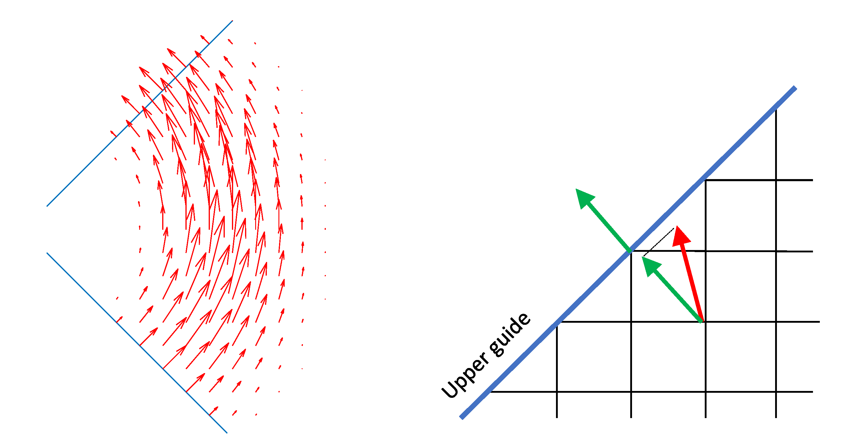
The boundaries are placed at a 45 degrees angle; thus, the imposition of the constraints comes very naturally. Neumann boundary conditions for the electric field are imposed on the antenna guide. This is done by respecting the perfect conductivity relation. Again referring to Figure 6 (right), at each time-step, the (red) vector of components $(E_r,E_z)$ in proximity of the boundary is projected onto the direction normal to the surface, giving birth to the (green) vector $\frac{1}{2}(E_r-E_z,E_z-E_r)$. This last vector is successively shifted up to the corresponding boundary grid point.

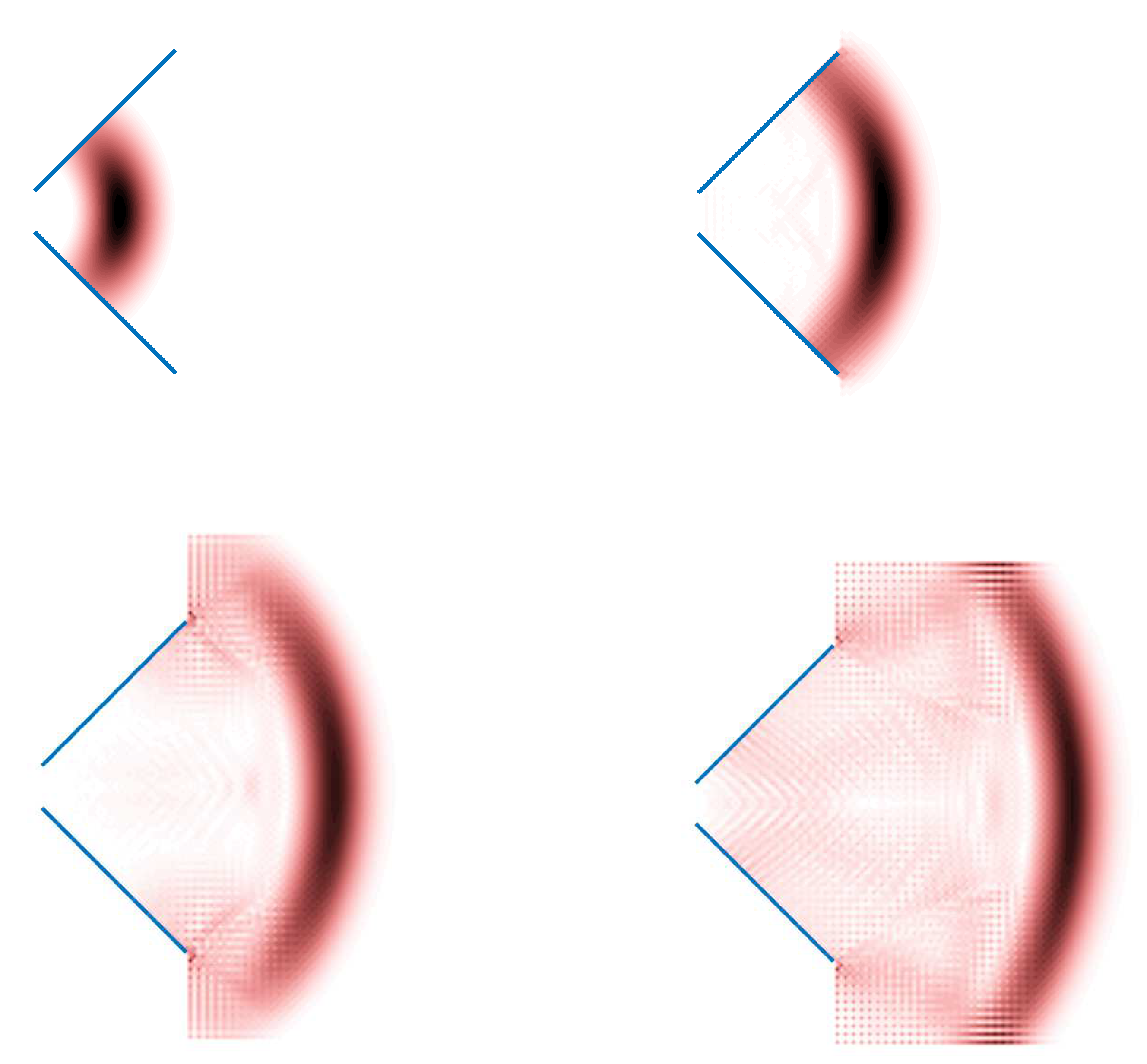
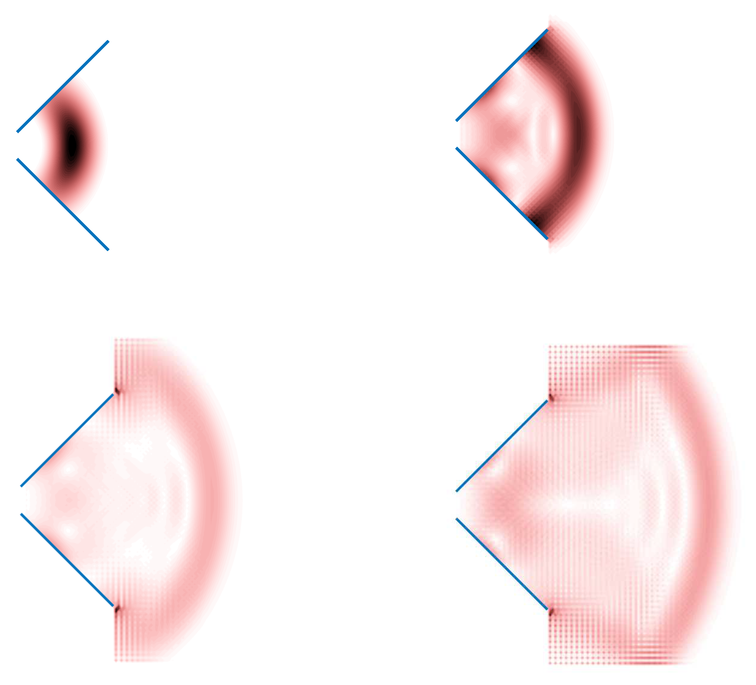
The parameters relative to the numerical tests are provided in the figure captions. As far as Figure 7 is concerned, the simulations rely on the field $\mathit{V}$ given in the first plot of Figure 5. At the grid points where $\mathit{V}$ is not defined, we are actually solving the system (6) and (7) with $\mathit{V}=0$. At the end of the guide the solution turns out to be discontinuous, thereby producing sensible numerical instabilities. The general behavior of the wave is however reasonably well reproduced.

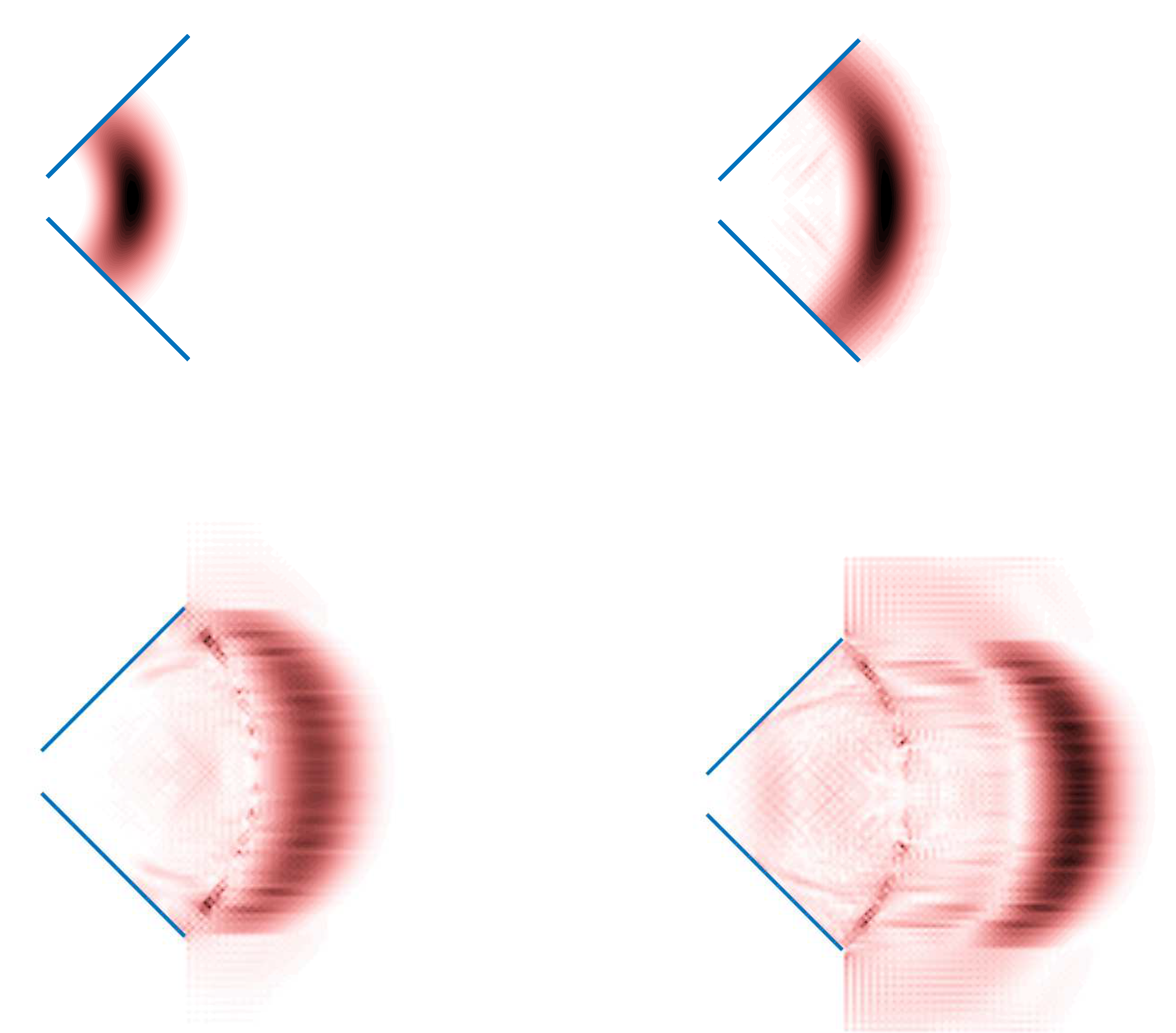
Concerning Figure 8, this is obtained from the field $\mathit{V}$ as given in the second plot of Figure 5. Again we set $\mathit{V}=0$ at the remaining grid points. The solution is clearly focused in the horizontal direction. The approximation suffers from the discontinuity across the dielectric boundary. Improvements could be obtained through the adoption of a more accurate discretization scheme. Anyway, our purpose here was to show that numerical simulations are feasible and produce a consistent prediction.

Finally, in Figure 9, we show the results when $\mathit{V}$ is totally eliminated. We are not, however, enforcing the condition $\rho =\nabla ·\mathit{E}=0$. Since the initial guess itself does not satisfy $\rho =0$, we cannot claim that we are actually solving the full set of Maxwell’s equations in a vacuum. We are not even solving the classical wave equation, since we can just deduce that: ${\partial }^2\mathit{E}/\partial t^2=-c^2\nabla \times (\nabla \times \mathit{E})=c^2(\Delta \mathit{E}-\nabla \rho )$. On the other hand, there are very few initial data recoverable from (24) such that $\rho =0$. This is true, for instance, for $g=1/sin\vartheta$, which does not correspond with a consistent choice for a signal emerging from an antenna (see the discussion in [14], Chapter 1).

The behavior of the solution shown in Figure 9, especially regarding the second plot (to be compared with the second plot of Figure 7), is very inefficient. As far as the successive plots are concerned, some of the energy remains concentrated at the endpoints of the guide. Noticeably, in most of the computational code available on the market, the checking of the zero divergence condition in vacuum is disregarded. This means that, if $\rho$ at a certain time starts assuming nonvanishing values (because of imposing some boundary constraints deriving for example from a scattering object), the problem is not approached in the proper way. This is true, for instance, in the case of Yee’s scheme, mentioned in Section 6, whose implementation strictly trusts the fact that $\rho$ must remain zero for all times. The real trouble is that Maxwell’s equations are too restrictive. In short, the solution of the vector wave equation, in a given domain with generic boundary conditions, has no chance to have its divergence be zero. That is why we adopted the extended model in our simulations.

We end this section with a few remarks. We placed our initial guess at a distance from the real source (the gap between the two cones). In truth, we do not exactly know how the signal is actually created (by going backwards the initial guess degenerates into a singularity). This uncertainty is a consequence of the fact that the mechanism of antenna emission is still not completely clear. First of all, the guides should not be assumed to be perfect conductors, a property that involves a nontrivial discussions about boundary conditions and the way they should be approximated (see, e.g., [29,30,31]). Such more complicated situations activate the whole set of modeling equations. In fact, we start with missing the orthogonality between $\mathit{E}$ and $\mathit{V}$. This generates values of the potential p different from zero, influencing in this way all the other variables. Secondly, there is a resonance process (depending on the size and shape of the device) that allows for the propagation of waves only if they are above a certain frequency. These issues are just sketched in this paper and are often underestimated in the design of a device. A transmitting antenna is an object transforming a certain signal by conferring to it the capability to travel in free space without further help from the source (see the final comments in the preliminary paper [32]). We believe that applied physics necessitates a better theoretical understanding of the mechanism of antenna emissions. Indeed, more accurate computations cannot neglect this crucial aspect.

9. Highly Directional Emissions

The computations of Section 8 have been realized for a relative permittivity coefficient ${\epsilon }_r\approx 2$, corresponding, for instance, with polyethylene. This is in fact the material that we would like to use in laboratory experiments, due to the possibility of shaping the dielectric through a 3D printing process.

A further conical metal reflector can be added to the device of Figure 2, obtaining the final antenna schematically represented in Figure 10. The angle at the vertex of the reflector is again $\pi /2$. In this way, the horizontally spreading signal is driven in the vertical direction. Referring to Figure 1, during the whole process, an annular wave starts inside the dielectric following a path like that shown in the central picture. When exiting the dielectric, the new Poynting vectors are lined up to the vectors $\mathit{V}$, as depicted in the picture on the right-hand side of Figure 1. Finally, after the last reflection, the signal is converted into a highly directional beam, such as that of the picture on the left-hand side of Figure 1.

During all these transitions there is no breaking of the stream lines of the magnetic field, which remain closed curves encircling the z-axis. After projection on the plane orthogonal to the z-axis, the evolution of the wave displays a central symmetry. This peculiar property is not commonly shared by other devices—for example, parabolic reflectors (when the source is represented by a classical dipole) or horn antennas. These devices actually need to break their initial symmetries in order to radiate [33].

Preliminary experiments without the presence of the dielectric showed that the signal emerging from the reflector has an annular shape. The fields are thus polarized in a sort of a circular fashion. The signal is absent nearby the z-axis. The global shape of the emitted wave is that of a torus. The directivity is relatively good, but, due to the lack of the dielectric lens correction, the toroidal wave grows with distance from the source, following a conical pattern. In those tests, the cones were replaced by two conductors having a complicated shape, in order to skip the construction of the dielectric medium $\Omega$. The outcome was interesting but still far from the directional signal we would like to achieve. The above experiments are however quite crucial in confirming some theoretical predictions. Waves as those just described do not exist in the Maxwellian framework. Indeed, the request that the divergence of the electric field must be always zero in a vacuum does not allow the inclusion of such special waves in the solution space. This means that the adoption of the revised model is rather important in the description of antennas already existing, opening the path to the design of a new generation of sustainable, efficient and performant devices.

It finally has to be noted that, if perfect directional signals exist, where the rays are all parallel, the natural receiver for this kind of antenna is the antenna itself. Indeed, as in a mirror image, the parallel rays are converted back and concentrated at the gap of the cones. There, they can be finally transformed in potentials.

10. Conclusions

We guessed the possibility of generating electromagnetic waves with extremely high directivity. This prediction is suggested by an extension of Maxwell’s equations in a vacuum aimed to simulate compact signals, traveling unperturbed at the speed of light. The enlargement of the solutions space relies on the fact that the divergence of the electric field may assume values different from zero also in the absence of charges associated with physical particles—for instance, electrons. This requirement is indeed able to explain many electromagnetic phenomena, as documented in [15]. In addition, the revised model provides the exact link between electrodynamics equations and the rules of geometrical optics, a property that the standard Maxwellian approach is not able to reproduce, unless one accepts a sequence of rough simplifications (see, e.g., [28], Section 3.1).

The waves belonging to the category we studied in this paper display a toroidal topology, with the magnetic field distributed along closed lines following the toroidal axis. With the help of simple devices, it is actually possible to create waves having a similar topology and developing along conical patterns. These emanations cannot be described by the classical Maxwell equation, so that the adoption of the extended model becomes a necessity dictated by reality.

The theory predicts that antennas with infinite directivity could possibly be built. Reality is a different issue, so reasonable quantitative confirmations will only be made as the results of the first experiments are made available. Once it is demonstrated that such a project is feasible, generating these waves becomes only matter of technical effort. The reader can of course understand the importance of this achievement. In this paper, we indicated a way to fabricate antennas devoted to this purpose. These are obtained by filling the space delimited by a biconic antenna with a dielectric medium placed in contact with the cones, and such that the boundary between the medium and the external vacuum is designed following a suitable curvature. The specific signals produced are expected to reach a prescribed target without dissipating their energy along the path. Moreover, since most of the theoretical passages are based on the rules of geometrical optics, we argue that the role of frequency might not be so crucial, thereby allowing transmissions ranging within a rather broad band. All these properties should guarantee a number of positive outcomes in terms of sustainable operation, safe energy transfer and secure information beaming.