Groundwater Spring Potential Mapping Using Artificial Intelligence Approach Based on Kernel Logistic Regression, Random Forest, and Alternating Decision Tree Models

 ,
, 
 ,
,  ,
, 
Abstract
1. Introduction
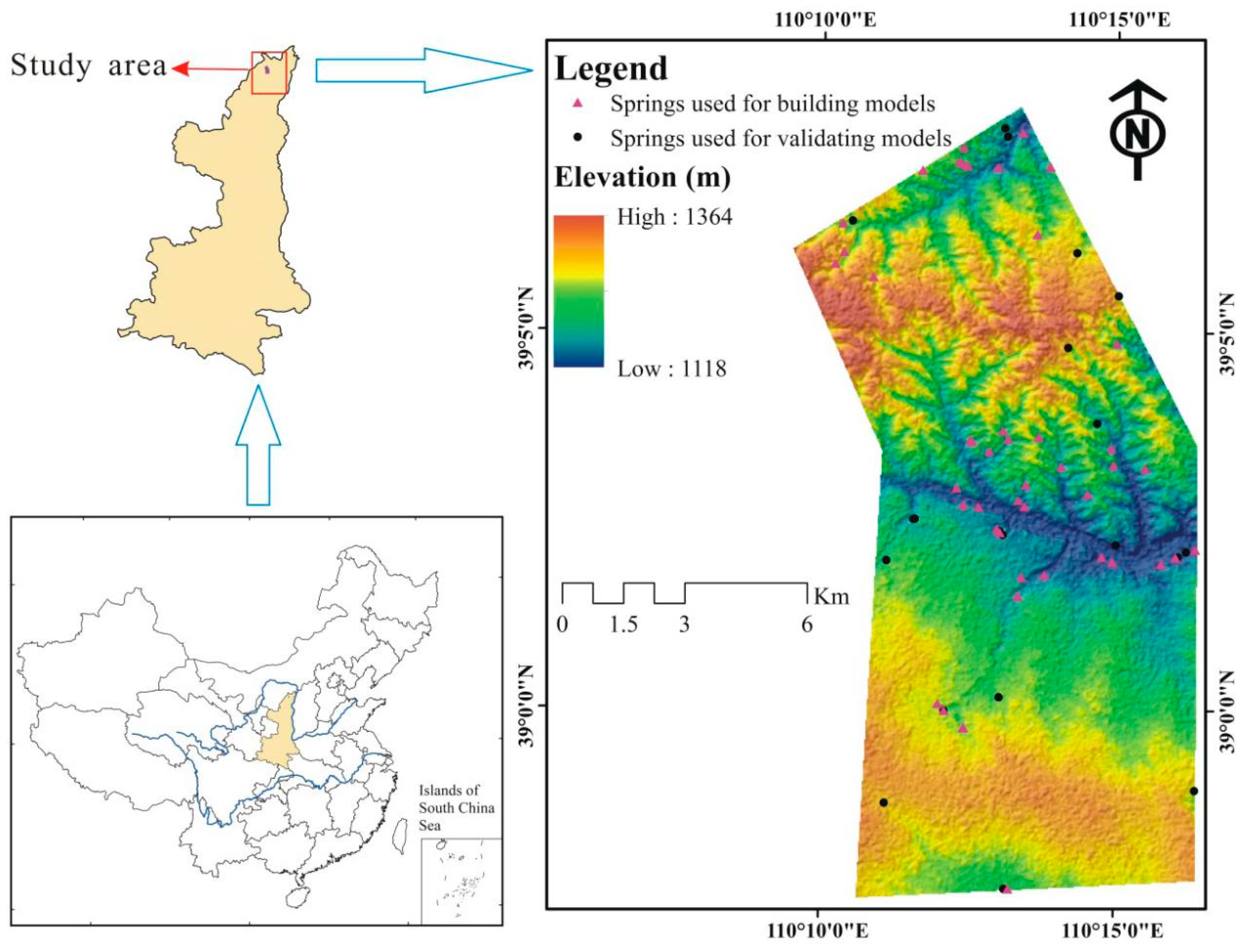
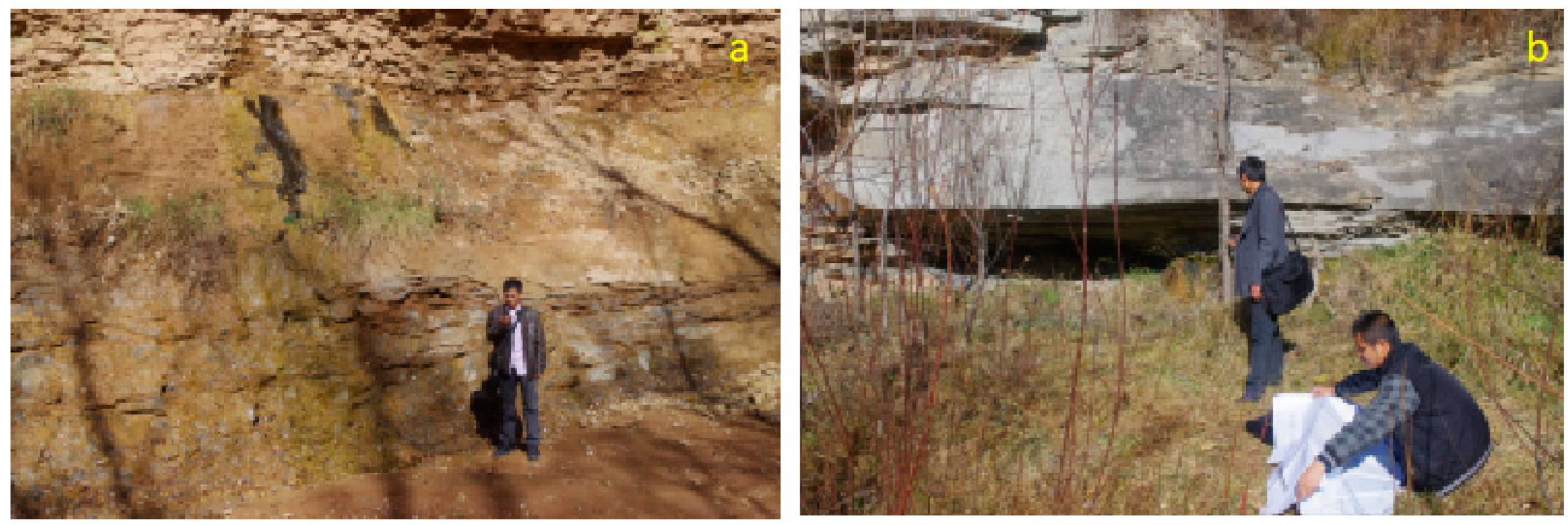
2. Study Area
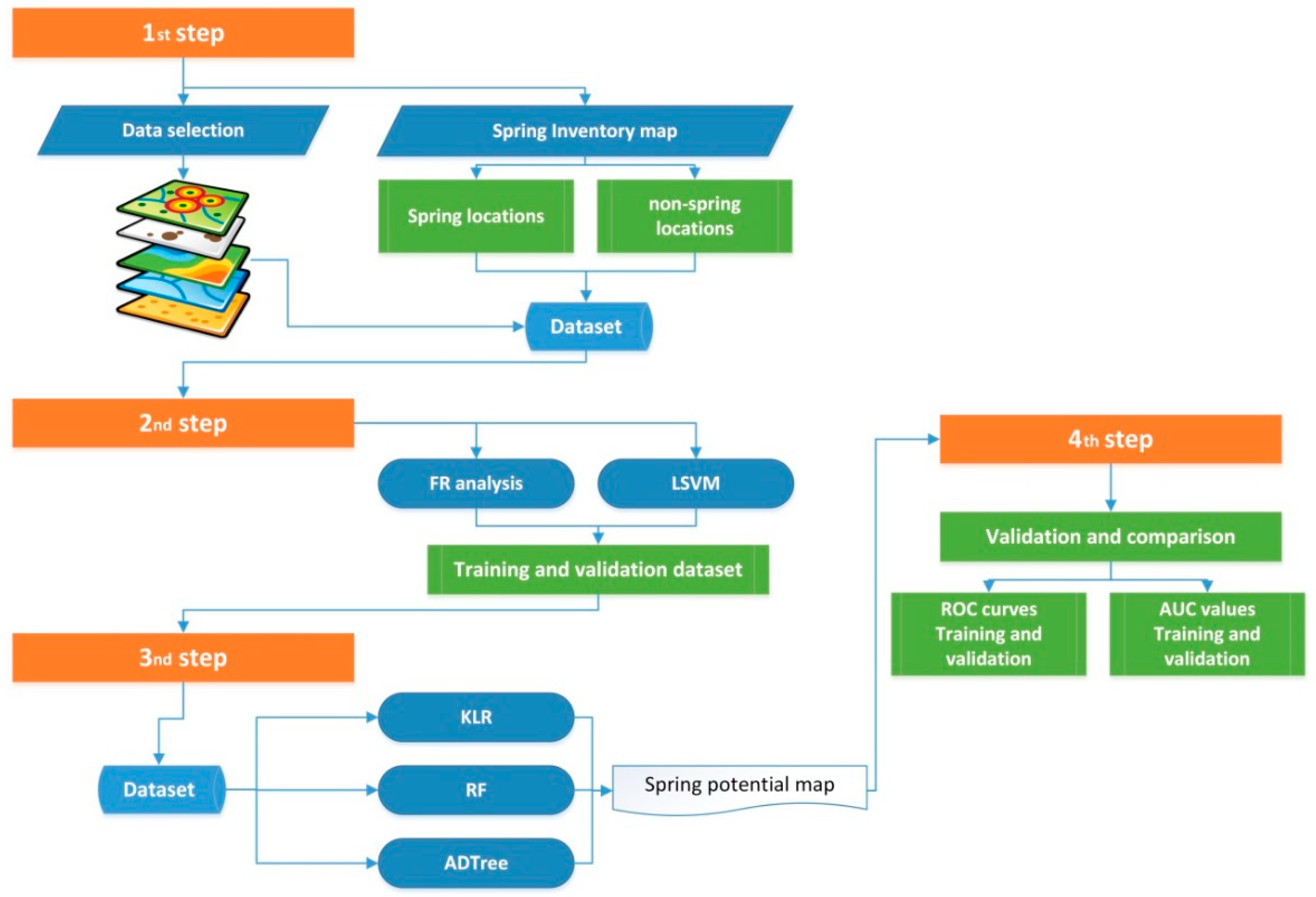
3. Methodology
3.1. Frequency Ratio (FR)
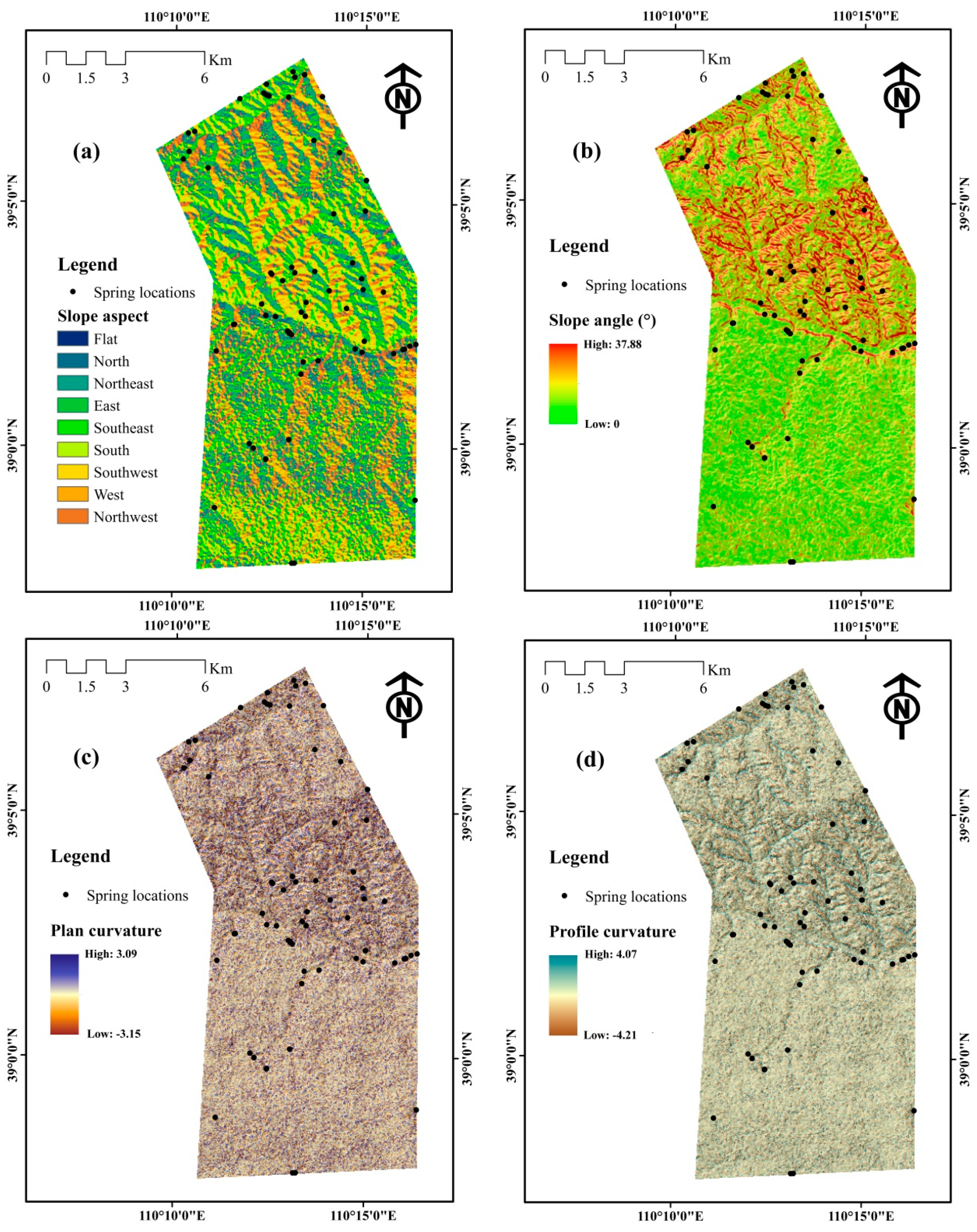
3.2. Selection of Spring Explanatory Factors Using an SVM Classifier
3.3. Kernel Logistic Regression (KLR)
3.4. Random Forest (RF)
3.5. Alternating Decision Tree (ADTree)
3.6. Validation and Comparison of the Results Obtained by the Models
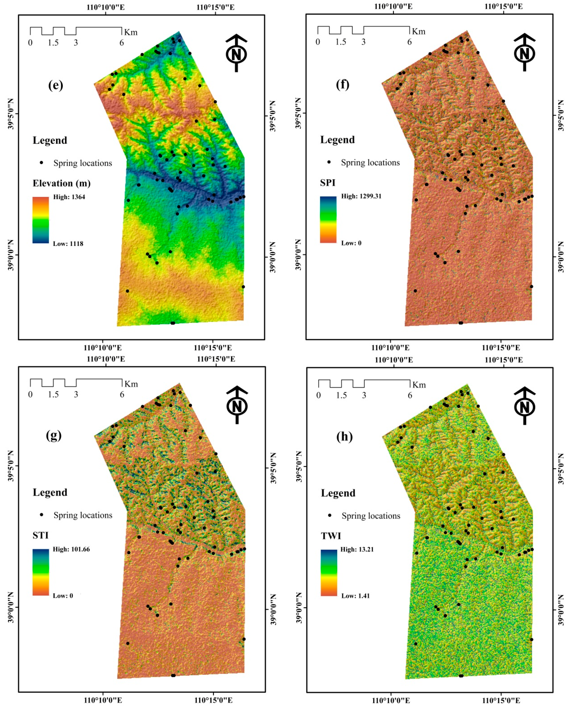
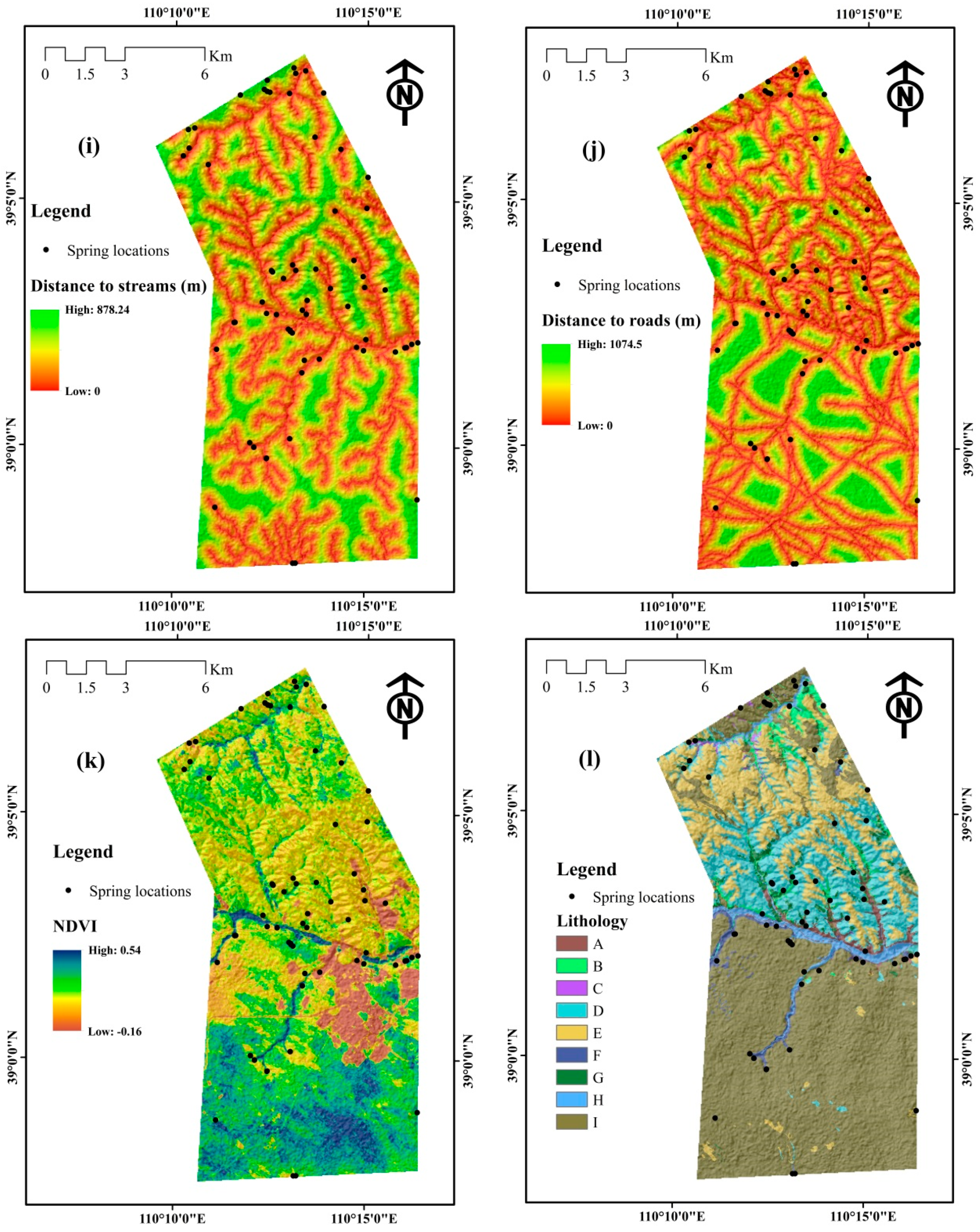
4. Data Used
5. Results
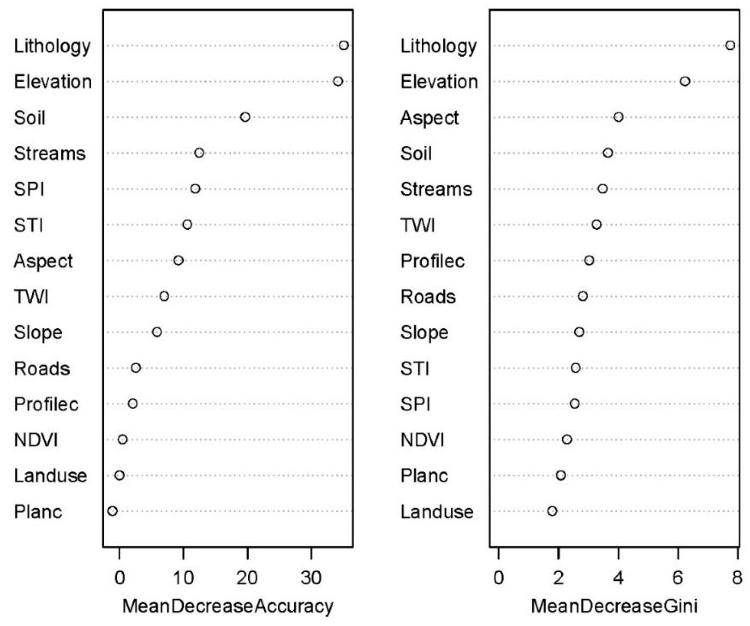
5.1. Results of Explanatory Factors Selection
5.2. Correlation Analysis between Springs and Explanatory Factors Using FR
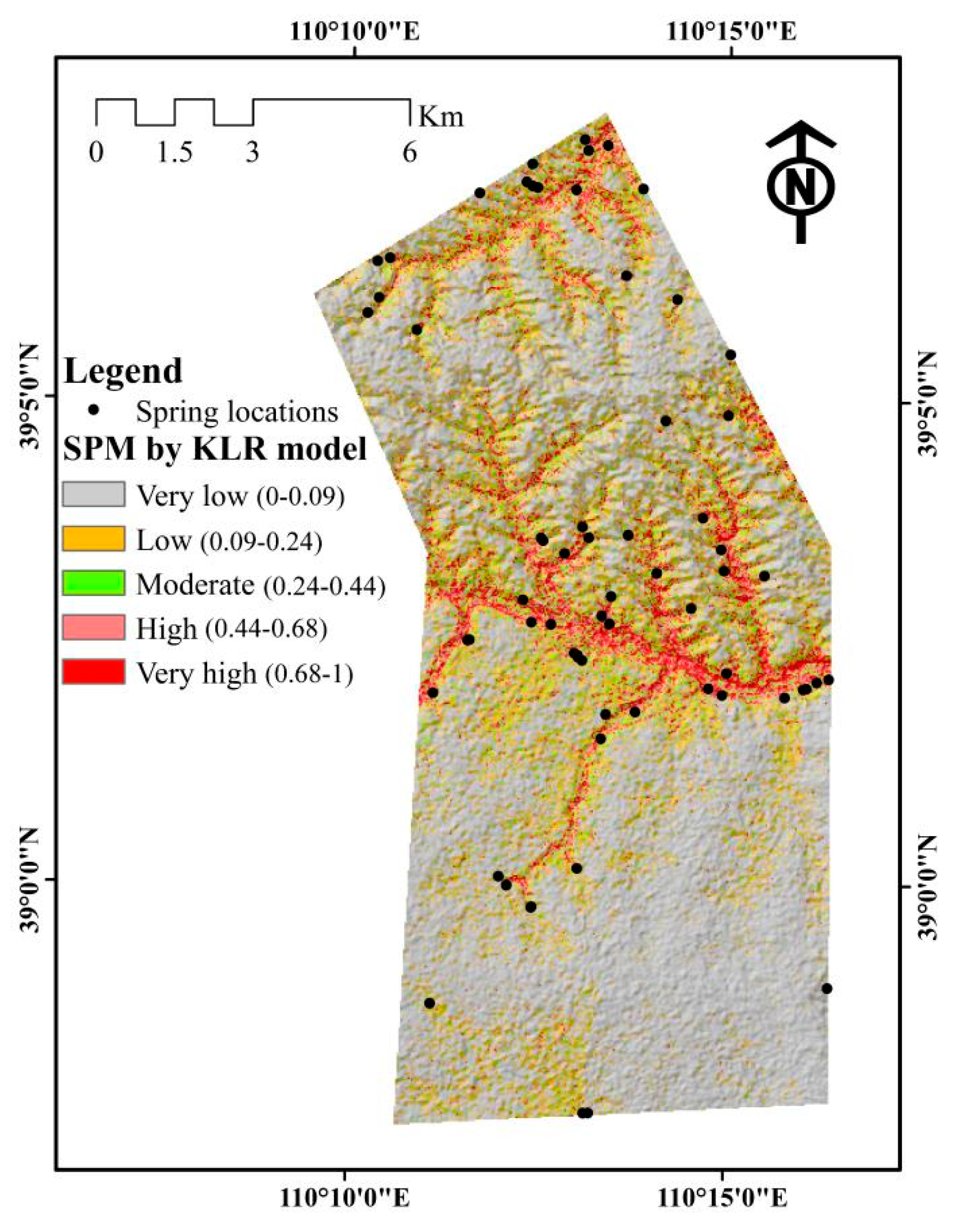
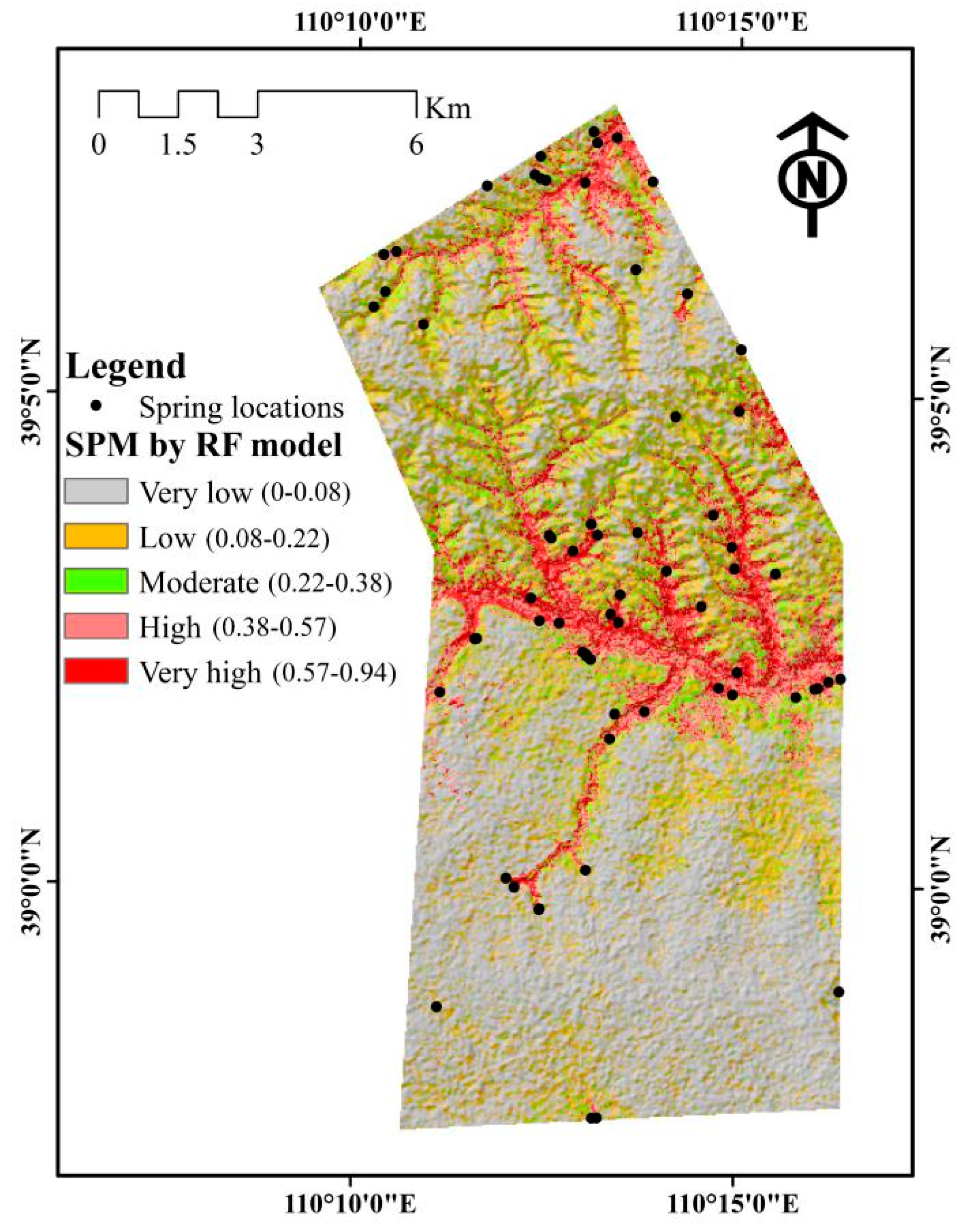
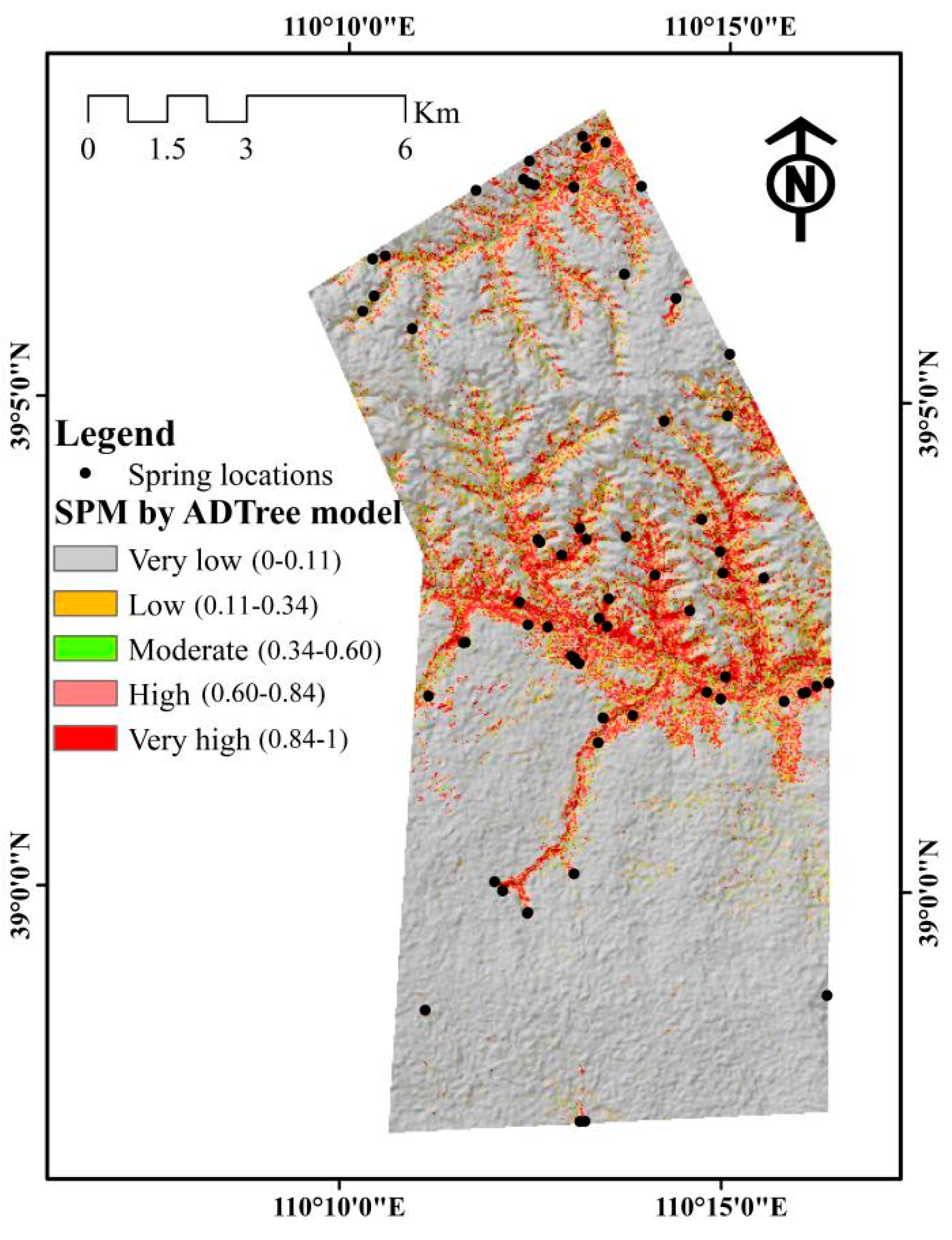
5.3. Application of KLR, RF, and ADTree Models
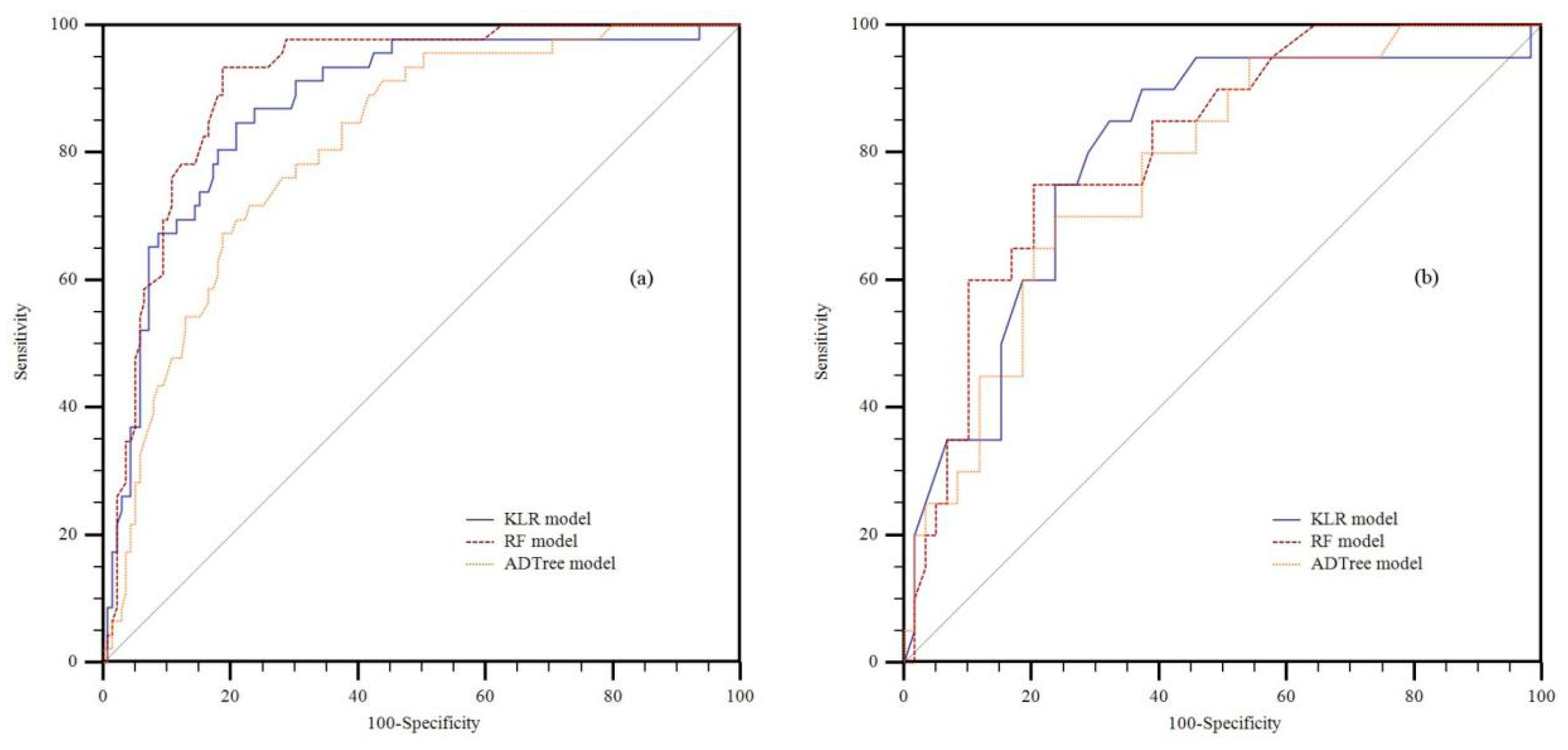
5.4. Validation and Comparison
6. Discussion
7. Conclusions
Author Contributions
Funding
Acknowledgments
Conflicts of Interest
References
- Ayazi, M.H.; Pirasteh, S.; Arvin, A.; Pradhan, B.; Nikouravan, B.; Mansor, S. Disasters and risk reduction in groundwater: Zagros mountain southwest Iran using geoinformatics techniques. Disaster Adv. 2010, 3, 51–57. [Google Scholar]
- Neshat, A.; Pradhan, B.; Pirasteh, S.; Shafri, H.Z.M. Estimating groundwater vulnerability to pollution using a modified drastic model in the Kerman agricultural area, Iran. Environ. Earth Sci. 2014, 71, 3119–3131. [Google Scholar] [CrossRef]
- Gleeson, T.; Befus, K.M.; Jasechko, S.; Luijendijk, E.; Cardenas, M.B. The global volume and distribution of modern groundwater. Nat. Geosci. 2016, 9, 161. [Google Scholar] [CrossRef]
- Rahmati, O.; Naghibi, S.A.; Shahabi, H.; Bui, D.T.; Pradhan, B.; Azareh, A.; Rafiei-Sardooi, E.; Samani, A.N.; Melesse, A.M. Groundwater spring potential modelling: Comprising the capability and robustness of three different modeling approaches. J. Hydrol. 2018, 565, 248–261. [Google Scholar] [CrossRef]
- De Vries, J.J.; Simmers, I. Groundwater recharge: An overview of processes and challenges. Hydrogeol. J. 2002, 10, 5–17. [Google Scholar] [CrossRef]
- Jackson, R.B.; Carpenter, S.R.; Dahm, C.N.; McKnight, D.M.; Naiman, R.J.; Postel, S.L.; Running, S.W. Water in a changing world. Ecol. Appl. 2001, 11, 1027–1045. [Google Scholar] [CrossRef]
- Rosegrant, M.W.; Cai, X. Global water demand and supply projections: Part 2. Results and prospects to 2025. Water Int. 2002, 27, 170–182. [Google Scholar] [CrossRef]
- Ercin, A.E.; Hoekstra, A.Y. Water footprint scenarios for 2050: A global analysis. Environ. Int. 2014, 64, 71–82. [Google Scholar] [CrossRef]
- Kummu, M.; Guillaume, J.; de Moel, H.; Eisner, S.; Flörke, M.; Porkka, M.; Siebert, S.; Veldkamp, T.I.; Ward, P.J. The world’s road to water scarcity: Shortage and stress in the 20th century and pathways towards sustainability. Sci. Rep. 2016, 6, 38495. [Google Scholar] [CrossRef] [PubMed]
- Kaushal, S.; Gold, A.; Mayer, P. Land Use, Climate, and Water Resources—Global Stages of Interaction; Multidisciplinary Digital Publishing Institute: Basel, Switzerland, 2017. [Google Scholar]
- Curran, S.R.; De Sherbinin, A. Completing the picture: The challenges of bringing “consumption” into the population–environment equation. Popul. Environ. 2004, 26, 107–131. [Google Scholar] [CrossRef]
- Naghibi, S.A.; Dashtpagerdi, M.M. Evaluation of four supervised learning methods for groundwater spring potential mapping in Khalkhal region (Iran) using GIS-based features. Hydrogeol. J. 2017, 25, 169–189. [Google Scholar] [CrossRef]
- Oh, H.-J.; Kim, Y.-S.; Choi, J.-K.; Park, E.; Lee, S. Gis mapping of regional probabilistic groundwater potential in the area of Pohang city, Korea. J. Hydrol. 2011, 399, 158–172. [Google Scholar] [CrossRef]
- Udimal, T.B.; Jincai, Z.; Ayamba, E.C.; Owusu, S.M. China’s water situation; the supply of water and the pattern of its usage. Int. J. Sustain. Built Environ. 2017, 6, 491–500. [Google Scholar] [CrossRef]
- Chen, W.; Panahi, M.; Khosravi, K.; Pourghasemi, H.R.; Rezaie, F.; Parvinnezhad, D. Spatial prediction of groundwater potentiality using anfis ensembled with teaching-learning-based and biogeography-based optimization. J. Hydrol. 2019, 572, 435–448. [Google Scholar] [CrossRef]
- Chen, W.; Tsangaratos, P.; Ilia, I.; Duan, Z.; Chen, X. Groundwater spring potential mapping using population-based evolutionary algorithms and data mining methods. Sci. Total Environ. 2019, 684, 31–49. [Google Scholar] [CrossRef] [PubMed]
- Moghaddam, D.D.; Rezaei, M.; Pourghasemi, H.; Pourtaghie, Z.; Pradhan, B. Groundwater spring potential mapping using bivariate statistical model and GIS in the Taleghan watershed, Iran. Arab. J. Geosci. 2015, 8, 913–929. [Google Scholar] [CrossRef]
- Corsini, A.; Cervi, F.; Ronchetti, F. Weight of evidence and artificial neural networks for potential groundwater spring mapping: An application to the Mt. Modino area (Northern Apennines, Italy). Geomorphology 2009, 111, 79–87. [Google Scholar] [CrossRef]
- Naghibi, S.A.; Pourghasemi, H.R. A comparative assessment between three machine learning models and their performance comparison by bivariate and multivariate statistical methods in groundwater potential mapping. Water Resour. Manag. 2015, 29, 5217–5236. [Google Scholar] [CrossRef]
- Chowdhury, A.; Jha, M.; Chowdary, V.; Mal, B. Integrated remote sensing and GIS-based approach for assessing groundwater potential in west Medinipur district, west Bengal, India. Int. J. Remote Sens. 2009, 30, 231–250. [Google Scholar] [CrossRef]
- Jha, M.K.; Bongane, G.M.; Chowdary, V. Groundwater potential zoning by remote sensing, GIS and mcdm techniques: A case study of eastern India. In Hydroinformatics in Hydrology, Hydrogeology and Water Resources, Proceedings of the Symposium JS. 4 at the Joint Convention of the International Association of Hydrological Sciences (IAHS) and the International Association of Hydrogeologists (IAH) held in Hyderabad, Hyderabad, India, 6–12 September 2009; IAHS Press: Wallingford, UK, 2009; pp. 432–441. [Google Scholar]
- Kumar, U.; Kumar, B.; Mallick, N. Groundwater prospects zonation based on RS and GIS using fuzzy algebra in Khoh river watershed, Pauri-Garhwal district, Uttarakhand, India. Glob. Perspect. Geogr. (GPG) 2013, 1, 37–45. [Google Scholar]
- Pourtaghi, Z.S.; Pourghasemi, H.R. GIS-based groundwater spring potential assessment and mapping in the Birjand Township, Southern Khorasan province, Iran. Hydrogeol. J. 2014, 22, 643–662. [Google Scholar] [CrossRef]
- Machiwal, D.; Jha, M.K.; Mal, B.C. Assessment of groundwater potential in a semi-arid region of India using remote sensing, GIS and MCDM techniques. Water Resour. Manag. 2011, 25, 1359–1386. [Google Scholar] [CrossRef]
- Adiat, K.; Nawawi, M.; Abdullah, K. Assessing the accuracy of GIS-based elementary multi criteria decision analysis as a spatial prediction tool—A case of predicting potential zones of sustainable groundwater resources. J. Hydrol. 2012, 440, 75–89. [Google Scholar] [CrossRef]
- Rahmati, O.; Samani, A.N.; Mahdavi, M.; Pourghasemi, H.R.; Zeinivand, H. Groundwater potential mapping at Kurdistan region of Iran using analytic hierarchy process and GIS. Arab. J. Geosci. 2015, 8, 7059–7071. [Google Scholar] [CrossRef]
- Shekhar, S.; Pandey, A.C. Delineation of groundwater potential zone in hard rock terrain of India using remote sensing, geographical information system (GIS) and analytic hierarchy process (AHP) techniques. Geocarto Int. 2015, 30, 402–421. [Google Scholar] [CrossRef]
- Lee, S.; Kim, Y.-S.; Oh, H.-J. Application of a weights-of-evidence method and GIS to regional groundwater productivity potential mapping. J. Environ. Manag. 2012, 96, 91–105. [Google Scholar] [CrossRef]
- Al-Abadi, A.M. Groundwater potential mapping at northeastern Wasit and Missan governorates, Iraq using a data-driven weights of evidence technique in framework of GIS. Environ. Earth Sci. 2015, 74, 1109–1124. [Google Scholar] [CrossRef]
- Nampak, H.; Pradhan, B.; Manap, M.A. Application of GIS based data driven evidential belief function model to predict groundwater potential zonation. J. Hydrol. 2014, 513, 283–300. [Google Scholar] [CrossRef]
- Mogaji, K.; Omosuyi, G.; Adelusi, A.; Lim, H. Application of GIS-based evidential belief function model to regional groundwater recharge potential zones mapping in Hardrock geologic terrain. Environ. Process. 2016, 3, 93–123. [Google Scholar] [CrossRef]
- Tahmassebipoor, N.; Rahmati, O.; Noormohamadi, F.; Lee, S. Spatial analysis of groundwater potential using weights-of-evidence and evidential belief function models and remote sensing. Arab. J. Geosci. 2016, 9, 79. [Google Scholar] [CrossRef]
- Kordestani, M.D.; Naghibi, S.A.; Hashemi, H.; Ahmadi, K.; Kalantar, B.; Pradhan, B. Groundwater potential mapping using a novel data-mining ensemble model. Hydrogeol. J. 2019, 27, 211–224. [Google Scholar] [CrossRef]
- Kim, K.-D.; Lee, S.; Oh, H.-J.; Choi, J.-K.; Won, J.-S. Assessment of ground subsidence hazard near an abandoned underground coal mine using GIS. Environ. Geol. 2006, 50, 1183–1191. [Google Scholar] [CrossRef]
- Ozdemir, A. Using a binary logistic regression method and GIS for evaluating and mapping the groundwater spring potential in the sultan mountains (Aksehir, Turkey). J. Hydrol. 2011, 405, 123–136. [Google Scholar] [CrossRef]
- Naghibi, S.A.; Pourghasemi, H.R.; Dixon, B. GIS-based groundwater potential mapping using boosted regression tree, classification and regression tree, and random forest machine learning models in Iran. Environ. Monit. Assess. 2016, 188, 44. [Google Scholar] [CrossRef] [PubMed]
- Zabihi, M.; Pourghasemi, H.R.; Pourtaghi, Z.S.; Behzadfar, M. GIS-based multivariate adaptive regression spline and random forest models for groundwater potential mapping in Iran. Environ. Earth Sci. 2016, 75, 665. [Google Scholar] [CrossRef]
- Lee, S.; Song, K.-Y.; Kim, Y.; Park, I. Regional groundwater productivity potential mapping using a geographic information system (GIS) based artificial neural network model. Hydrogeol. J. 2012, 20, 1511–1527. [Google Scholar] [CrossRef]
- Kim, J.-C.; Jung, H.-S.; Lee, S. Groundwater productivity potential mapping using frequency ratio and evidential belief function and artificial neural network models: Focus on topographic factors. J. Hydroinform. 2018, 20, 1436–1451. [Google Scholar] [CrossRef]
- Lee, S.; Hong, S.-M.; Jung, H.-S. GIS-based groundwater potential mapping using artificial neural network and support vector machine models: The case of Boryeong city in Korea. Geocarto Int. 2018, 33, 847–861. [Google Scholar] [CrossRef]
- Aguilera, P.A.; Fernández, A.; Ropero, R.F.; Molina, L. Groundwater quality assessment using data clustering based on hybrid Bayesian networks. Stoch. Environ. Res. Risk Assess. 2013, 27, 435–447. [Google Scholar] [CrossRef]
- Naghibi, S.A.; Pourghasemi, H.R.; Abbaspour, K. A comparison between ten advanced and soft computing models for groundwater qanat potential assessment in Iran using R and GIS. Theor. Appl. Climatol. 2018, 131, 967–984. [Google Scholar] [CrossRef]
- Chen, W.; Li, H.; Hou, E.; Wang, S.; Wang, G.; Panahi, M.; Li, T.; Peng, T.; Guo, C.; Niu, C.; et al. GIS-based groundwater potential analysis using novel ensemble weights-of-evidence with logistic regression and functional tree models. Sci. Total Environ. 2018, 634, 853–867. [Google Scholar] [CrossRef] [PubMed]
- Khosravi, K.; Panahi, M.; Bui, D.T. Spatial prediction of groundwater spring potential mapping based on an adaptive neuro-fuzzy inference system and metaheuristic optimization. Hydrol. Earth Syst. Sci. 2018, 22, 4771–4792. [Google Scholar] [CrossRef]
- National Soil Survey Office. Chinese Soil Types; China Agricultural Press: Beijing, China, 1995. [Google Scholar]
- Nithya, N.S.; Duraiswamy, K. Gain ratio based fuzzy weighted association rule mining classifier for medical diagnostic interface. Sadhana 2014, 39, 39–52. [Google Scholar] [CrossRef][Green Version]
- Bui, D.T.; Tuan, T.A.; Hoang, N.-D.; Thanh, N.Q.; Nguyen, D.B.; Van Liem, N.; Pradhan, B. Spatial prediction of rainfall-induced landslides for the Lao Cai area (Vietnam) using a hybrid intelligent approach of least squares support vector machines inference model and artificial bee colony optimization. Landslides 2017, 14, 447–458. [Google Scholar]
- Guyon, I.; Weston, J.; Barnhill, S.; Vapnik, V. Gene selection for cancer classification using support vector machines. Mach. Learn. 2002, 46, 389–422. [Google Scholar] [CrossRef]
- Pham, B.T.; Bui, D.T.; Pourghasemi, H.R.; Indra, P.; Dholakia, M.B. Landslide susceptibility assesssment in the Uttarakhand area (India) using GIS: A comparison study of prediction capability of naïve bayes, multilayer perceptron neural networks, and functional trees methods. Theor. Appl. Climatol. 2015, 128, 1–19. [Google Scholar] [CrossRef]
- Chen, W.; Xie, X.; Wang, J.; Pradhan, B.; Hong, H.; Bui, D.T.; Duan, Z.; Ma, J. A comparative study of logistic model tree, random forest, and classification and regression tree models for spatial prediction of landslide susceptibility. Catena 2017, 151, 147–160. [Google Scholar] [CrossRef]
- Tanaka, K.; Kurita, T.; Kawabe, T. Selection of import vectors via binary particle swarm optimization and cross-validation for kernel logistic regression. In Proceedings of the 2007 International Joint Conference on Neural Networks, Orlando, FL, USA, 12–17 August 2007; pp. 1037–1042. [Google Scholar]
- Mercer, J. Functions of Positive and Negative Type, and Their Connection with the Theory of Integral Equations; Royal Society of London Philosophical Transactions: London, UK, 1909; Volume 209, pp. 415–446. [Google Scholar]
- Bui, D.T.; Tuan, T.A.; Klempe, H.; Pradhan, B.; Revhaug, I. Spatial prediction models for shallow landslide hazards: A comparative assessment of the efficacy of support vector machines, artificial neural networks, kernel logistic regression, and logistic model tree. Landslides 2016, 13, 361–378. [Google Scholar]
- Jo, T.; Cheng, J. Improving protein fold recognition by random forest. BMC Bioinform. 2014, 15, 1–7. [Google Scholar] [CrossRef]
- Ravìa, D.; Bober, M.; Farinella, G.M.; Guarnera, M.; Battiato, S. Semantic segmentation of images exploiting dct based features and random forest. J. Pain Palliat. Care Pharmacother. 2015, 24, 429. [Google Scholar] [CrossRef]
- Breiman, L. Random forest. Mach. Learn. 2001, 45, 5–32. [Google Scholar] [CrossRef]
- Freund, Y.; Mason, L. The alternating decision tree learning algorithm. In Proceedings of the Sixteenth International Machine Learning Conference, Bled, Slovenia, 27–30 June 1999; Morgan Kaufmann: San Francisco, CA, USA, 2002; pp. 124–133. [Google Scholar]
- Buntine, W. Learning classification trees. Stat. Comput. 1992, 2, 63–73. [Google Scholar] [CrossRef]
- Kohavi, R.; Kunz, C. Option decision trees with majority votes. In Proceedings of the Fifteenth International Machine Learning Conference (ICML 1998), Madison, MI, USA, 24–27 July 1998. [Google Scholar]
- Min, S.L.; Oh, S. Alternating decision tree algorithm for assessing protein interaction reliability. Vietnam J. Comput. Sci. 2014, 1, 169–178. [Google Scholar]
- Hosseinalizadeh, M.; Kariminejad, N.; Chen, W.; Pourghasemi, H.R.; Alinejad, M.; Mohammadian Behbahani, A.; Tiefenbacher, J.P. Gully headcut susceptibility modeling using functional trees, naïve bayes tree, and random forest models. Geoderma 2019, 342, 1–11. [Google Scholar] [CrossRef]
- Chen, W.; Hong, H.; Panahi, M.; Shahabi, H.; Wang, Y.; Shirzadi, A.; Pirasteh, S.; Alesheikh, A.A.; Khosravi, K.; Panahi, S.; et al. Spatial prediction of landslide susceptibility using GIS-based data mining techniques of anfis with whale optimization algorithm (WOA) and grey wolf optimizer (GWO). Appl. Sci. 2019, 9, 3755. [Google Scholar] [CrossRef]
- Chen, W.; Li, Y.; Xue, W.; Shahabi, H.; Li, S.; Hong, H.; Wang, X.; Bian, H.; Zhang, S.; Pradhan, B.; et al. Modeling flood susceptibility using data-driven approaches of naïve bayes tree, alternating decision tree, and random forest methods. Sci. Total Environ. 2020, 701, 134979. [Google Scholar] [CrossRef]
- Chen, W.; Fan, L.; Li, C.; Pham, B.T. Spatial prediction of landslides using hybrid integration of artificial intelligence algorithms with frequency ratio and index of entropy in Nanzheng county, China. Appl. Sci. 2020, 10, 29. [Google Scholar] [CrossRef]
- Zhao, X.; Chen, W. GIS-based evaluation of landslide susceptibility models using certainty factors and functional trees-based ensemble techniques. Appl. Sci. 2020, 10, 16. [Google Scholar] [CrossRef]
- Yesilnacar, E.; Topal, T. Landslide susceptibility mapping: A comparison of logistic regression and neural networks methods in a medium scale study, Hendek region (Turkey). Eng. Geol. 2005, 79, 251–266. [Google Scholar] [CrossRef]
- Chen, W.; Shahabi, H.; Zhang, S.; Khosravi, K.; Shirzadi, A.; Chapi, K.; Pham, B.; Zhang, T.; Zhang, L.; Chai, H. Landslide susceptibility modeling based on GIS and novel bagging-based kernel logistic regression. Appl. Sci. 2018, 8, 2540. [Google Scholar] [CrossRef]
- Chen, W.; Sun, Z.; Han, J. Landslide susceptibility modeling using integrated ensemble weights of evidence with logistic regression and random forest models. Appl. Sci. 2019, 9, 171. [Google Scholar] [CrossRef]
- ESRI. ArcGIS Desktop: Release 10.3.1; Environmental Systems Research Institute: Redlands, CA, USA, 2015. [Google Scholar]
- Cantonati, M.; Segadelli, S.; Ogata, K.; Tran, H.; Sanders, D.; Gerecke, R.; Rott, E.; Filippini, M.; Gargini, A.; Celico, F. A global review on ambient Limestone-Precipitating Springs (LPS): Hydrogeological setting, ecology, and conservation. Sci. Total Environ. 2016, 568, 624–637. [Google Scholar] [CrossRef] [PubMed]
- Hou, E.; Wang, J.; Chen, W. A comparative study on groundwater spring potential analysis based on statistical index, index of entropy and certainty factors models. Geocarto Int. 2018, 33, 754–769. [Google Scholar] [CrossRef]
- Ayalew, L.; Yamagishi, H. The application of GIS-based logistic regression for landslide susceptibility mapping in the Kakuda-Yahiko Mountains, Central Japan. Geomorphology 2005, 65, 15–31. [Google Scholar] [CrossRef]
- Zeinivand, H.; Ghorbani Nejad, S. Application of GIS-based data-driven models for groundwater potential mapping in Kuhdasht region of Iran. Geocarto Int. 2018, 33, 651–666. [Google Scholar] [CrossRef]
- Chen, W.; Xie, X.; Peng, J.; Wang, J.; Duan, Z.; Hong, H. GIS-based landslide susceptibility modelling: A comparative assessment of kernel logistic regression, naïve-bayes tree, and alternating decision tree models. Geomat. Nat. Hazards Risk 2017, 8, 950–973. [Google Scholar] [CrossRef]
- Chen, W.; Pourghasemi, H.R.; Naghibi, S.A. Prioritization of landslide conditioning factors and its spatial modeling in Shangnan county, China using GIS-based data mining algorithms. Bull. Eng. Geol. Environ. 2018, 77, 611–629. [Google Scholar] [CrossRef]
- Williams, G. Data Mining with Rattle and R: The Art of Excavating Data for Knowledge Discovery; Springer Science & Business Media: Berlin, Germany, 2011. [Google Scholar]
- Chen, W.; Hong, H.; Li, S.; Shahabi, H.; Wang, Y.; Wang, X.; Ahmad, B.B. Flood susceptibility modelling using novel hybrid approach of reduced-error pruning trees with bagging and random subspace ensembles. J. Hydrol. 2019, 575, 864–873. [Google Scholar] [CrossRef]
- Li, Y.; Chen, W. Landslide susceptibility evaluation using hybrid integration of evidential belief function and machine learning techniques. Water 2020, 12, 113. [Google Scholar] [CrossRef]
- Nagarajan, M.; Singh, S. Assessment of groundwater potential zones using GIS technique. J. Indian Soc. Remote Sens. 2009, 37, 69–77. [Google Scholar] [CrossRef]
- Ballukraya, P.; Kalimuthu, R. Quantitative hydrogeological and geomorphological analyses for groundwater potential assessment in hard rock terrains. Curr. Sci. 2010, 253–259. [Google Scholar]
- Chen, W.; Pradhan, B.; Li, S.; Shahabi, H.; Rizeei, H.M.; Hou, E.; Wang, S. Novel hybrid integration approach of bagging-based fisher’s linear discriminant function for groundwater potential analysis. Nat. Resour. Res. 2019, 28, 1239–1258. [Google Scholar] [CrossRef]
- Jaiswal, R.; Mukherjee, S.; Krishnamurthy, J.; Saxena, R. Role of remote sensing and GIS techniques for generation of groundwater prospect zones towards rural development—An approach. Int. J. Remote Sens. 2003, 24, 993–1008. [Google Scholar] [CrossRef]
- Madrucci, V.; Taioli, F.; de Araújo, C.C. Groundwater favorability map using GIS multicriteria data analysis on crystalline terrain, Sao Paulo state, Brazil. J. Hydrol. 2008, 357, 153–173. [Google Scholar] [CrossRef]
- Srivastava, P.K.; Bhattacharya, A.K. Groundwater assessment through an integrated approach using remote sensing, GIS and resistivity techniques: A case study from a hard rock terrain. Int. J. Remote Sens. 2006, 27, 4599–4620. [Google Scholar] [CrossRef]
- Cuo, L.; Giambelluca, T.W.; Ziegler, A.D.; Nullet, M.A. Use of the distributed hydrology soil vegetation model to study road effects on hydrological processes in Pang Khum Experimental Watershed, northern Thailand. For. Ecol. Manag. 2006, 224, 81–94. [Google Scholar] [CrossRef]
- Golkarian, A.; Naghibi, S.A.; Kalantar, B.; Pradhan, B. Groundwater potential mapping using c5.0, random forest, and multivariate adaptive regression spline models in GIS. Environ. Monit. Assess. 2018, 190, 149. [Google Scholar] [CrossRef]


| Categories | Codes | Lithologies |
|---|---|---|
| Group A | J2y | Mudstone, sandy mudstone, arcose sandstone |
| Group B | J2z | Mudstone, sandstone, glutenite |
| Group C | J2a | Mudstone, sandstone |
| Group D | N2b | Clay |
| Group E | Q2l | Loess |
| Group F | Q3s | Sand |
| Group G | Q3m | Loess |
| Group H | Q4al | Alluvium |
| Group I | Q4eol | Eolian deposit |
| No. | Explanatory Factors | AM | Standard Deviation |
|---|---|---|---|
| 1 | Lithology | 14.0 | ±0.000 |
| 2 | Elevation | 12.8 | ±0.400 |
| 3 | SPI | 12.2 | ±0.400 |
| 4 | Soil cover | 10.6 | ±0.490 |
| 5 | Distance to roads | 9.9 | ±0.831 |
| 6 | Slope aspect | 9.3 | ±0.900 |
| 7 | TWI | 7.4 | ±1.020 |
| 8 | Slope angle | 6.2 | ±1.327 |
| 9 | STI | 5.6 | ±1.685 |
| 10 | Land use | 4.9 | ±1.758 |
| 11 | Distance to streams | 4.7 | ±1.487 |
| 12 | Profile curvature | 3.0 | ±1.789 |
| 13 | Plan curvature | 2.5 | ±0.671 |
| 14 | NDVI | 1.9 | ±1.814 |
| Explanatory Factors | Classes | No. of Pixels in Domain | No. of Springs | FR |
|---|---|---|---|---|
| Slope aspect | Flat | 160 | 0 | 0.000 |
| North | 20,781 | 7 | 1.110 | |
| Northeast | 23,407 | 3 | 0.422 | |
| East | 18,904 | 5 | 0.871 | |
| Southeast | 16,567 | 10 | 1.989 | |
| South | 19,695 | 8 | 1.338 | |
| Southwest | 19,789 | 6 | 0.999 | |
| West | 15,924 | 3 | 0.621 | |
| Northwest | 16,327 | 4 | 0.807 | |
| Slope angle (°) | <5 | 61,434 | 9 | 0.483 |
| 5–10 | 52,808 | 20 | 1.248 | |
| 10–15 | 22,886 | 9 | 1.296 | |
| 15–20 | 10,114 | 6 | 1.955 | |
| 20–25 | 3368 | 2 | 1.956 | |
| 25–30 | 797 | 0 | 0.000 | |
| >30 | 147 | 0 | 0.000 | |
| Plan curvature | −3.15 to −0.77 | 7701 | 2 | 0.856 |
| −0.77 to −0.28 | 28,451 | 18 | 2.084 | |
| −0.28–0.11 | 55,026 | 7 | 0.419 | |
| 0.11–0.60 | 46,644 | 14 | 0.989 | |
| 0.60–3.09 | 13,732 | 5 | 1.200 | |
| Profile curvature | −4.21 to −0.74 | 9855 | 4 | 1.337 |
| −0.74 to −0.22 | 37,272 | 8 | 0.707 | |
| −0.22–0.20 | 56,394 | 14 | 0.818 | |
| 0.20–0.72 | 37,360 | 11 | 0.970 | |
| 0.72–4.07 | 10,673 | 9 | 2.778 | |
| Elevation (m) | <1150 | 1906 | 4 | 6.914 |
| 1150–1200 | 13,983 | 11 | 2.592 | |
| 1200–1250 | 46,890 | 22 | 1.546 | |
| 1250–1300 | 61,507 | 9 | 0.482 | |
| >1300 | 27,268 | 0 | 0.000 | |
| SPI | <10 | 112,248 | 29 | 0.851 |
| 10–20 | 18,612 | 3 | 0.531 | |
| 20–30 | 7174 | 2 | 0.918 | |
| 30–40 | 3641 | 5 | 4.524 | |
| >40 | 9879 | 7 | 2.335 | |
| STI | <2 | 83,093 | 16 | 0.634 |
| 2–4 | 31,339 | 12 | 1.262 | |
| 4–6 | 14,344 | 4 | 0.919 | |
| 6–8 | 8108 | 4 | 1.625 | |
| >8 | 14,670 | 10 | 2.246 | |
| TWI | <2 | 13,564 | 10 | 2.429 |
| 2–2.5 | 62,484 | 10 | 0.527 | |
| 2.5–3 | 43,231 | 13 | 0.991 | |
| 3–3.5 | 17,294 | 6 | 1.143 | |
| >3.5 | 14,981 | 7 | 1.539 | |
| Distance to streams (m) | <50 | 22,376 | 10 | 1.472 |
| 50–100 | 19,583 | 10 | 1.682 | |
| 100–150 | 18,591 | 6 | 1.063 | |
| 150–200 | 13,111 | 7 | 1.759 | |
| >200 | 77,893 | 13 | 0.550 | |
| Distance to roads (m) | <50 | 36,659 | 14 | 1.258 |
| 50–100 | 26,995 | 11 | 1.343 | |
| 100–150 | 22,234 | 6 | 0.889 | |
| 150–200 | 13,323 | 9 | 2.226 | |
| >200 | 52,343 | 6 | 0.378 | |
| NDVI | −0.16–0.04 | 10,165 | 4 | 1.296 |
| 0.04–0.13 | 50,750 | 18 | 1.169 | |
| 0.13–0.19 | 46,711 | 17 | 1.199 | |
| 0.19–0.26 | 33,496 | 3 | 0.295 | |
| 0.26–0.54 | 10,432 | 4 | 1.263 | |
| Lithology | A | 2275 | 4 | 5.793 |
| B | 4103 | 9 | 7.227 | |
| C | 495 | 1 | 6.656 | |
| D | 24,980 | 8 | 1.055 | |
| E | 26,024 | 4 | 0.506 | |
| F | 2271 | 7 | 10.155 | |
| G | 2895 | 3 | 3.414 | |
| H | 3653 | 1 | 0.902 | |
| I | 84,858 | 9 | 0.349 | |
| Soil | Calcari-Gypsiric Arenosols (Arc) | 67,657 | 10 | 0.487 |
| Haplic Arenosols (ARh) | 17,325 | 10 | 1.902 | |
| Calcareous red clay (CMe) | 8418 | 0 | 0.000 | |
| Luvi-Calcic Kastanozems (KSk) | 58,154 | 26 | 1.473 | |
| Land use | Farmland | 33,485 | 10 | 0.984 |
| Forest | 5148 | 0 | 0.000 | |
| Grass | 89,545 | 30 | 1.104 | |
| Water | 743 | 0 | 0.000 | |
| Residential areas | 13,036 | 2 | 0.505 | |
| Others | 9,597 | 4 | 1.373 |
| Classes | KLR (%) | RF (%) | ADTree (%) |
|---|---|---|---|
| Very low | 58.80 | 46.90 | 76.66 |
| Low | 18.91 | 21.57 | 5.90 |
| Moderate | 10.10 | 13.77 | 4.04 |
| High | 7.18 | 10.76 | 4.25 |
| Very High | 5.02 | 7.01 | 9.15 |
| Models | AUC | SE | 95% CI |
|---|---|---|---|
| KLR | 0.877 | 0.0294 | 0.821 to 0.921 |
| RF | 0.909 | 0.0225 | 0.858 to 0.946 |
| ADTree | 0.812 | 0.0341 | 0.748 to 0.866 |
| Models | AUC | SE | 95% CI |
|---|---|---|---|
| KLR | 0.797 | 0.0591 | 0.691 to 0.879 |
| RF | 0.811 | 0.0526 | 0.707 to 0.890 |
| ADTree | 0.773 | 0.0578 | 0.665 to 0.860 |
© 2020 by the authors. Licensee MDPI, Basel, Switzerland. This article is an open access article distributed under the terms and conditions of the Creative Commons Attribution (CC BY) license (http://creativecommons.org/licenses/by/4.0/).
Share and Cite
Chen, W.; Li, Y.; Tsangaratos, P.; Shahabi, H.; Ilia, I.; Xue, W.; Bian, H. Groundwater Spring Potential Mapping Using Artificial Intelligence Approach Based on Kernel Logistic Regression, Random Forest, and Alternating Decision Tree Models. Appl. Sci. 2020, 10, 425. https://doi.org/10.3390/app10020425
Chen W, Li Y, Tsangaratos P, Shahabi H, Ilia I, Xue W, Bian H. Groundwater Spring Potential Mapping Using Artificial Intelligence Approach Based on Kernel Logistic Regression, Random Forest, and Alternating Decision Tree Models. Applied Sciences. 2020; 10(2):425. https://doi.org/10.3390/app10020425
Chicago/Turabian StyleChen, Wei, Yang Li, Paraskevas Tsangaratos, Himan Shahabi, Ioanna Ilia, Weifeng Xue, and Huiyuan Bian. 2020. "Groundwater Spring Potential Mapping Using Artificial Intelligence Approach Based on Kernel Logistic Regression, Random Forest, and Alternating Decision Tree Models" Applied Sciences 10, no. 2: 425. https://doi.org/10.3390/app10020425
APA StyleChen, W., Li, Y., Tsangaratos, P., Shahabi, H., Ilia, I., Xue, W., & Bian, H. (2020). Groundwater Spring Potential Mapping Using Artificial Intelligence Approach Based on Kernel Logistic Regression, Random Forest, and Alternating Decision Tree Models. Applied Sciences, 10(2), 425. https://doi.org/10.3390/app10020425