A Comparative Evaluation of Nature Inspired Algorithms for Telecommunication Network Design

Abstract

The subject of the study was an application of nature-inspired metaheuristic algorithms to node configuration optimization in optical networks. The main objective of the optimization was to minimize capital expenditure, which includes the costs of optical node resources, such as transponders and amplifiers used in a new generation of optical networks. For this purpose a model that takes into account the physical phenomena in the optical network is proposed. Selected nature-inspired metaheuristic algorithms were implemented and compared with a reference, deterministic algorithm, based on linear integer programming. For the cases studied the obtained results show that there is a large advantage in using metaheuristic algorithms. In particular, the evolutionary algorithm, the bees algorithm and the harmony search algorithm showed superior performance for the considered data-sets corresponding to large optical networks; the integer programming-based algorithm failed to find an acceptable sub-optimal solution within the assumed maximum computational time. All optimization methods were compared for selected instances of realistic teletransmission networks of different dimensions subject to traffic demand sets extracted from real traffic data.

1. Introduction

From the network operator’s point of view, the ever-increasing demand for high-speed data services translates into the need to continually upgrade the networks to increase the data transmission rate per optical fiber. An engineer who is responsible for the task of continual upgrading of dense wavelength division multiplexing (DWDM) networks [1] needs specific software tools that allow for estimation of the network’s performance and optimization of the architecture with respect to operational and capital costs. Thus, the specific task considered in this contribution related to DWDM network optimization was formulated as an integer programming (IP) problem and solved by the available general purpose solvers [2]. However, the IP optimization results show that even if the IP approach is applicable, it is inefficient for larger networks since the design task is, in general, NP-complete [3]. The numerical efficiency limitations are particularly acute in the context of routing and wavelength assignment (RWA) [4,5,6] and routing and spectrum allocation (RSA) [7,8,9,10] problems, which are at the heart of DWDM network optimization. Moreover, the constraints and cost functions are in a general case nonlinear and thus may further complicate the situation.

Since the invention of computationally efficient exact algorithms is rather unlikely, heuristic discrete optimization methods seem to be best suited for the optimization of DWDM networks with realistic size and high modularity of node resources while taking into account optical network impairments, such as attenuation or an optical signal to noise ratio (OSNR) [11,12]. Therefore, the main aim of this paper is to study the properties of heuristic algorithms that are applicable to the optimization of DWDM networks, whereby particular attention is paid to nature-inspired algorithms, with problem-specific operators that were specifically adapted by the authors to the problem studied. The performances of all optimization algorithms were compared for selected test networks with differing complexity. All networks used for comparison were optimized, subject to traffic demand sets extracted from real traffic data [13].

This paper is organized as follows. In Section 2 the problem is formulated and the network models are described. Due to space constraints we decided to keep the presentation of the problem to a minimum and refer to our previous article. In Section 3 general methodology is described. In Section 4 the proposed metaheuristics are described. Next, in Section 5 a testbed of four network structures is presented and results of series of numerical experiments testing the algorithms are provided and compared. Finally, Section 6 provides a summary of the research findings.

2. Problem Formulation

In this section, the UW-WDM network optimization problem is formulated using MIP [10]. For this purpose the following sets are defined:

$\mathcal{N}$

set of all nodes;

$\mathcal{T}$

set of transponders;

$\mathcal{S}$

set of frequency slices;

$\mathcal{E}$

set of edges;

${\mathcal{P}}_{(n,n^{\prime },t)}$

set of paths between nodes $n,n^{\prime }\in \mathcal{N}$ for transponder $t\in \mathcal{T}$; $p\subseteq \mathcal{E}$;

$\mathcal{B}$

set of bands;

${\mathcal{S}}_b$

set of frequency slices used by band $b\in \mathcal{B}$; ${\mathcal{S}}_b\subseteq \mathcal{S}$; ${\displaystyle \bigcup _{b\in \mathcal{B}}}{\mathcal{S}}_b=\mathcal{S}$;

${\mathcal{S}}_t$

set of frequency slices that can be used as starting; slices for transponder $t\in \mathcal{T}$; ${\mathcal{S}}_t\subseteq \mathcal{S}$.

Notice that the power budget constraints are taken into account in the model by limiting sets ${\mathcal{P}}_{(n,n^{\prime },t)}$. In this approach, the sets are precomputed and contain only paths that are feasible from the point of view of the power budget.

We use the following variables:

$y_{be}$

binary variable, equal to 1 if band b is used on edge e and 0 otherwise;

$x_{tn{n}^{\prime }ps}$

binary variable that equals 1 if transponders t are installed between node n and node $n^{\prime }$, routed on path p and start on frequency slice $s\in {\mathcal{S}}_t$, and 0 otherwise.

In the model, the following constants are used:

$\xi \left(b\right)$

cost of using band b at a single edge;

$\xi (t,b)$

cost of using a pair of transponders t in band b;

$v\left(t\right)$

bitrate provided by transponder t;

$d(n,n^{\prime })$

bitrate demanded from node n to node $n^{\prime }$;

$u(t,s,s^{\prime })$

binary constant that equals 1 if transponder t using bandwidth starting at frequency slice s also uses frequency slice $s^{\prime }$; 0 otherwise.

In the cost model EDFAs, preamplifiers, boosters, ILAs and transponders are included in $\xi \left(b\right)$ and $\xi (t,b)$ but not WSSs and filters since the latter devices cannot be subject to optimization.

The optimization model is as follows:

$$\begin{array}{c}min\sum _{b\in \mathcal{B}}\left(\xi \left(b\right)\sum _{e\in \mathcal{E}}{y}_{be}+\sum _{t\in \mathcal{T}}\xi (t,b)\sum _{n,n^{\prime }\in \mathcal{N}}\sum _{p\in {\mathcal{P}}_{(n,n^{\prime },t)}}\sum _{s\in {\mathcal{S}}_t}{x}_{tn{n}^{\prime }ps}\right)\end{array}$$

(1)

$$\begin{array}{c}\sum _{t\in \mathcal{T}}\sum _{p\in {\mathcal{P}}_{(n,n^{\prime },t)}}\sum _{s\in {\mathcal{S}}_t}v\left(t\right)x_{tn{n}^{\prime }ps}\ge d(n,n^{\prime })\forall n,n^{\prime }\in \mathcal{N}\end{array}$$

(2)

$$\begin{array}{c}\sum _{t\in \mathcal{T}}\sum _{n,n^{\prime }\in \mathcal{N}}\sum _{p\in {\mathcal{P}}_{(n,n^{\prime },t)}:e\in p}\sum _{s\in {\mathcal{S}}_t}u(t,s,s^{\prime })·x_{tn{n}^{\prime }ps}\le y_{be}\forall e\in \mathcal{E},\forall b\in \mathcal{B},\forall s^{\prime }\in {\mathcal{S}}_b\end{array}$$

(3)

The subject of minimization is the cost of installed amplifiers and transponders in (1). Constraints (2) ensure that all demands are satisfied. Constraints (3) ensure that each frequency slice at each edge is not used more than once. Moreover, they ensure that using a band at an edge results in installing appropriate amplifiers.

In this contribution the CAPEX minimization problem is considered and several techniques are applied in order to reduce the calculation time. The motivation for reducing the calculation time of the CAPEX minimization problem is two fold. First of all the CAPEX minimization should be performed each time new capacity is needed following a request coming from a customer. Hence, smaller calculation time is of clear benefit. Secondly, it was observed that the calculation time of standard optimization methods (e.g., ILP) growths rapidly with the number of network nodes [7]. Thus, for large networks, application of heuristic methods becomes indispensable.

3. Methodology

3.1. Solution Model

For each algorithm the same solution model was applied. The generic structure of the solution model is shown in Figure 1. Thus, in order to implement an algorithm, the following steps are taken:

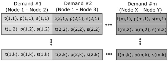
Figure 1. Structure of a model. Each demand consists of k 3-element vectors; k may be different for different demands.

• For all node pairs in set $\mathcal{N}$, a set of transponders $\mathcal{T}$ must be selected that are capable of meeting the demands for the node pair. The set is a 4-element vector $\mathcal{T}=\{n·t_1,n·t_2,n·t_3,n·t_4\}$, where the first element is the number of 40G transponders used, the second element is the number of 100 G transponders used, the third element is the number of 200 G transponders used and fourth element is the number of 400 G transponders used. For example, $\mathcal{T}=\{2,1,0,3\}$ means that this set consists of two 40 G transponders, one 100 G transponder and three 400 Gb transponders. The set of transponders is chosen from four precalculated solutions, generated using linear programming.
• For each selected transponder a path should be determined, through which it will transmit data. The path $p\in \mathcal{P}$ is selected randomly by drawing one of the k-element set of predefined paths.
• Choosinga path is necessary to be able to assign each transponder $t\in \mathcal{T}$ a unique piece of bandwidth $s\in \mathcal{S}$ for data transmission. This is done using a heuristic RMLSA (routing modulation level and spectrum allocation) algorithm [14] that sequentially handles each demand and uses longest path first (LPF) sorting.

3.2. Operators

This section shortly describes operators used to modify a solution, i.e., change realization operator, change path operator, crossover operator.

Operator change realization operator calculates a new solution for a given demand. For each demand we precalculate four sets of transponders capable of satisfying them. After choosing one of the precalculated sets, for each transponder $t\in \mathcal{T}$ of the set one of the predefined paths is randomly chosen.

Operator change path operator changes a path assigned to a transponder. A new path is randomly chosen from a set of predefined paths. Thus change path operator changes the selected path identifier allocated to the specific transponder to a random allowed value. Thus, if k paths are available, then change path operator changes the path identifier to a randomly selected value taken from a set of $\{1,2,\dots ,k\}$. In this study for each demand, $k=3$ was assumed.

For implementation of crossover operator, a uniform crossover [15] was used. In this application offspring chromosomes are created as a concatenation of demand vectors picked up randomly from parents. In this variant of crossover, the C genotype is formed from the parents’ genes on the basis of the following scheme:

$$C_i=\left\{\begin{array}{cc}{A}_i\hfill & {\zeta }_i<p_e\hfill \\ B_i\hfill & \mathrm{otherwise},\hfill \end{array}\right.$$

where ${\zeta }_i$ means the execution of a random variable with a $U(0,1)$ uniform distribution, drawn for each i item in the genotype separately, and $p_e$ is the probability of gene replacement. A typical $p_e$ value is: $p_e=\frac{1}{2}$. An example of the crossover, based on Polish network is depicted in Figure 2. In this specific example, the demand-two vector is subject to crossover, i.e., demand two for offspring has been swapped when compared to parents.

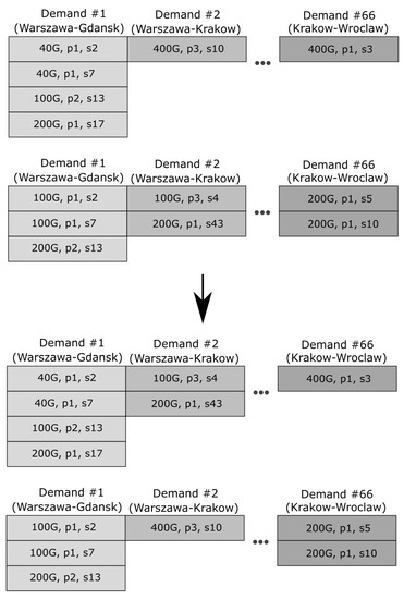
Figure 2. An example of crossover, based on the Polish network.

4. Methods

In the paper, several methods were used to solve the problem presented in Section 2, which can be divided into two classes. The first class is formed by population algorithms and consists of the bees algorithm (BA) [16,17,18] and the evolutionary algorithm (EA) [19,20,21]. The second class consists of algorithms that generate one solution in each iteration. Here, the harmony search algorithm (HS) [22] and the stochastic hill climbing algorithm (HC) [23] were considered. As the reference a well-known method based on integer linear programming (IP) was used [24,25]. This method is available through a commercial solver CPLEX [2].

4.1. The Bees Algorithm

The bees algorithm is inspired by honey bees and their way of searching for flower patches rich in nectar [16]. Each solution and its value of the objective function might be perceived as a flower patch found by a scout-bee and amount of nectar available there. The neighborhood of a flower patch rich in nectar should be explored by more bees than the other flower patches. Initially, the search space is randomly sampled according to scout bees randomly searching the surroundings of the hive. Thus N random solutions are generated. Then, a group of m best solutions is chosen from the current population. These solutions are used for local search. For the elite e out of m solutions $n_1$ random neighbors are generated. Analogously, for the remaining best $m-e$ solutions $n_2$ random neighbors are generated.

Note that $n_1$ should be greater than $n_2$ and the size of the neighborhood of local search is determined by value k. To generate a neighbor, change realization operator is used k times. At the end of each iteration m best solutions are chosen from best, elite and newly generated neighbors. To keep the population size constant, the current populations is filled with $N-m$ completely random solutions. The pseudo-code of the algorithm is presented in Algorithm 1. For the problem described in this article the hyperparameters N, m, e, $n_1$, $n_2$, k should be relatively small.

Algorithm 1: The bees algorithm.

4.2. Harmony Search

At the beginning of the algorithm the memory harmony is initialized [26]. It is set of randomly generated and evaluated solution models. The size of the memory is constant. In each iteration a new solution is created using the following steps:

• For each node pair in set $\mathcal{N}$ choose solution which satisfies the demand.
• With probability $p_a$, a solution is chosen randomly from memory. There is also probability $p_m$ that the chosen solution will be modified using change path operator.
• Otherwise, a solution is created using change realization operator.

After creation, the solution is evaluated and if it is better than any of the solutions stored in the memory, the worst solution is replaced by the newly created solution. Due to two ways of generating solutions, the algorithm has the option to explore and exploit solution space. Furthermore, it is certain that the best solution generated will be the final solution because of the way of storing solutions in memory. The pseudo-code of the algorithm is presented in Algorithm 2.

Algorithm 2: Harmony search.

4.3. Evolutionary Algorithm

The EA, which was employed for the optical node optimization problem, was inspired by evolutionary strategy (($\mu +\lambda$) ES) given in [27,28], but both the encoding method and genetic operators that were applied here are problem-specific. Its pseudo-code is given in Algorithm 3.

The algorithm maintains a population $P_t$ of individuals. The population is initialized randomly. For each gene, the demand that is associated with it is randomly allocated to a possible path. Then the objective function of each individual is calculated according to (1). The main loop of the algorithm works for the specified number of iterations, which is a parameter of the method. Inside the main loop, an offspring population $O_t$ is generated by reproducing randomly selected elements from $P_t$. Then, chromosomes are randomly mated into pairs, crossed over and mutated. A new population $P_{t+1}$ is generated by selecting best chromosomes from the sum of the base population and the offspring population.

To be able to use the EA, the solution of the problem must be encoded to form a genotype of an individual. The structure of the chromosome has already been depicted in Figure 1 and an example of the chromosome based on Polish network is depicted in Figure 3. Demand 1 is realized by means of four transponders (first, traversing path 1 and using slice 2; second, 40 G traversing the same path, using slice 7; third, 100 G transponder-path 2 and slice 13; and fourth, 200 G transponder–path 1 and slice 17). Demand 2 has two transponders and the last demand 66 has just one transponder, traversing path 1, using slice 5. The crossover is performed using crossover operator as described earlier. The mutation is performed for each chromosome. Each demand is mutated separately with probability $p_m$ using change path operator.

Algorithm 3: The evolutionary algorithm ($\mu +\lambda$)–EA.

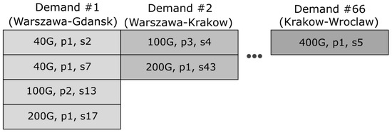
Figure 3. An example of a chromosome, based on Polish network.

5. Results and Discussion

Computational results were obtained for seven optical networks that have different characteristics. The networks correspond to actual optical networks stemming from specified countries and were taken from [29]. Table 1 and Figure 4, Figure 5, Figure 6, Figure 7, Figure 8, Figure 9 and Figure 10 provide the relevant parameters for both networks and their topologies.

Table 1. Parameters of analyzed networks.

Network	#Nodes	#Links	#Demands
Germany10	10	14	45
Polish	12	18	66
Germany15	15	23	105
Germany20	20	29	190
USA	26	42	325
American	39	61	741
Germany	50	88	1225

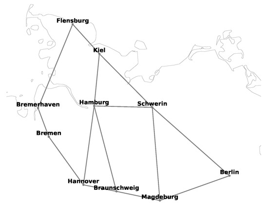
Figure 4. Schematic diagram of 10-node German national transmission optical backbone network.

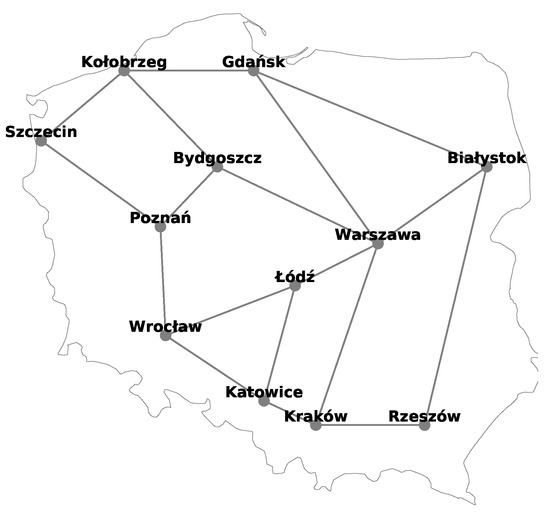
Figure 5. Schematic diagram of Polish national transmission optical backbone network.

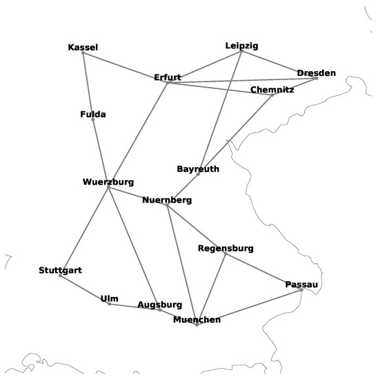
Figure 6. Schematic diagram of 15-node German national transmission optical backbone network.

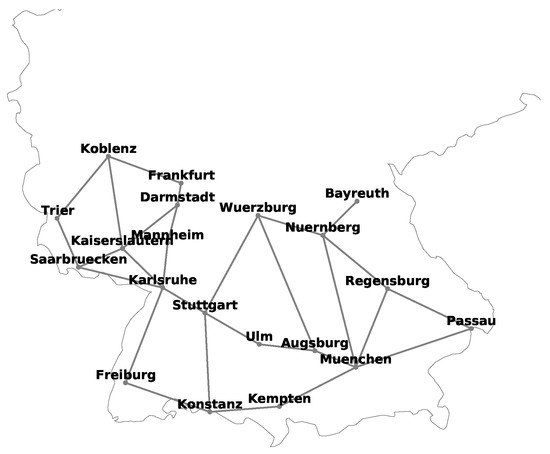
Figure 7. Schematic diagram of 20-node German national transmission optical backbone network.

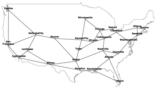
Figure 8. Schematic diagram of a USA national transmission optical backbone network.

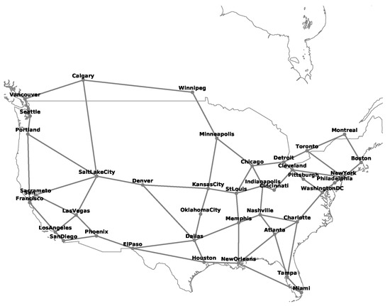
Figure 9. Schematic diagram of an American national transmission optical backbone network.

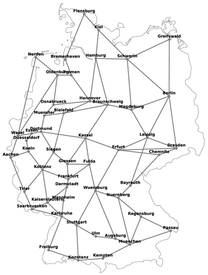
Figure 10. Schematic diagram of 50-node German national transmission optical backbone network.

The demands that were used in the optimization of network costs are given by a demand matrix, which provides the values of traffic flow between selected nodes expressed in gigabits per second (Gbps). The calculations were carried out using a linear solver engine of CPLEX 12.8.0.0 on a 2.1 GHz Xeon E7-4830 v.3 processor with 256 GB RAM running under Linux Debian operating system. Table 2 describes in detail the sets and their settings and presents constant settings used during the computational process.

Table 2. Set and constant settings.

Set	Set Settings
$\mathcal{N}$	in Table 1
$\mathcal{E}$	in Table 1
$\mathcal{S}$	768 slots
$\mathcal{B}$	2 bands
$\mathcal{T}$	4 transponders ($t_1=40$ G, $t_2=100$ G, $t_3=200$ G and $t_4=400$ G)
${\mathcal{S}}_t$	${\mathcal{S}}_1=\{1\cdots 380\}\cup \{385\cdots 764\}$ ${\mathcal{S}}_2=\{1\cdots 380\}\cup \{385\cdots 762\}$ ${\mathcal{S}}_3=\{1\cdots 378\}\cup \{385\cdots 762\}$ ${\mathcal{S}}_4=\{1\cdots 376\}\cup \{385\cdots 760\}$
Constant	Constant Settings
$d(n,n^{\prime })$[Gbps]	e.g., $d(1,2)=70$
$\xi \left(b\right)$	$\xi \left(1\right)=1$, $\xi \left(2\right)=2$
$\xi (t,b)$	$\xi (1,1)=2$, $\xi (2,1)=5$, $\xi (3,1)=7$, $\xi (4,1)=9$ $\xi (1,2)=2.4$, $\xi (2,2)=6$, $\xi (3,2)=8.4$, $\xi (4,2)=11.8$

The following modeling parameters were used for heuristic algorithms: $p_a=0.95$, $p_m=0.05$ and $memory\_size=30$ for HS; $N=50$, $m=12$, $e=6$, $n_1=8$, $n_2=2$ and $k=5$ for BA; and $\mu =100$$\lambda /\mu =2$, $p_c=0.9$ and $p_m=0,05$ for EA. All these values were selected empirically after a series of tests.

In the first numerical experiment a comparison of optimization methods was performed. For Polish, German10, German15 and German20 networks (Figure 4, Figure 5, Figure 6 and Figure 7 and Figure 11), which are discussed first, all considered algorithms reached the optimal solution. Results of heuristic algorithms are characterized by a small standard deviation. This observation supports the claim that the simulations are quite repetitive and that they converge consistently to effectively the same value. Further, the results from Table 3, Table 4, Table 5 and Table 6 show that average values are close to the minimum values. This is particularly the case for the BA algorithm. Thus, BA algorithm showed on average the best performance among all heuristic algorithms in terms of consistency.

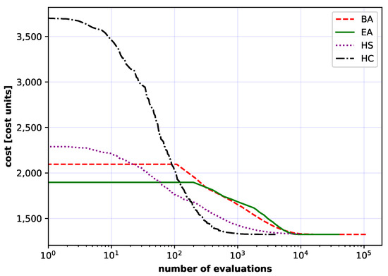
Figure 11. Comparison of the convergence for the Polish network of all considered methods: artificial bee colony (BA), evolutionary algorithm (EA), harmony search algorithm (HS) and stochastic hill climbing algorithm (HC). Each curve is an average of 50 independent runs.

Table 3. Comparison of all considered algorithms for the 10-node German network.

	German10
Method	Solution			#Evaluation	Time [sec.]
	Best	Mean	std. dev.	Mean	Mean	std. dev.	Gap [%]
BA	152	152.63	0.48	69,992	6990.8	170.7	–
EA	152	152.59	0.49	21,220	2170.0	51.0	–
HS	152	152.96	0.19	5293	529.18	25.86	–
HC	153	153.96	0.19	5226	522.18	25.86	–
IP	152	–	–	–	461.12	–	0.00

Table 4. Comparison of all considered algorithms for the Polish network.

	Polish
Method	Solution			#Evaluation	Time [sec.]
	Best	Mean	std. dev.	Mean	Mean	std. dev.	Gap [%]
BA	1321	1321.0	0.0	108,000	7650.8	165.2	–
EA	1321	1321.6	1.3	40,000	8562.1	275.3	–
HS	1321	1330.1	5.9	7641	420.3	90.1	–
HC	1321	1321.7	1.4	2421	410.8	80.8	–
IP	1321	–	–	–	367.0	–	0.00

Table 5. Comparison of all considered algorithms for the 15-node German network.

	German15
Method	Solution			#Evaluation	Time [sec.]
	Best	Mean	std. dev.	Mean	Mean	std. dev.	Gap [%]
BA	281	281.85	0.35	70,084	7008.0	170.7	–
EA	281	281.4	0.49	27,220	2710.0	62.0	–
HS	281	281.93	0.47	5862	582.37	105.5	–
HC	282	282.9	0.32	5440	544.5	24.8	–
IP	281	–	–	–	1547.10	–	0.00

Table 6. Comparison of all considered algorithms for the 20-node German network.

	German20
Method	Solution			#Evaluation	Time [sec.]
	Best	Mean	std. dev.	Mean	Mean	std. dev.	Gap [%]
BA	500	502.1	0.21	55,612	5561.0	417.7	–
EA	500	506.0	0.70	29,770	2870.0	20.7	–
HS	501	503.7	0.4	5245	524.5	47.1	–
HC	501	504.0	0.3	6255	625.3	562.0	–
IP	500	–	–	–	17304.75	–	0.00

The results obtained by HS algorithm on the other hand, are characterized by the highest standard deviation and the highest average value of the cost function. Thus, HS algorithm performed worst among all heuristic algorithms. It is also important to note that CPLEX software took about 6 min to find the optimal solution of 1321. Therefore, on average, IP approach won the competition for the Polish network instance. Finally, it is noted that on average, the fastest heuristic algorithm turned out to be HC algorithm. A bit worse, in terms of time, was the HS algorithm. Both of these algorithms were close to the IP approach in terms of time. The swarm algorithms (BA and EA) finally reached the optimum, but needed about 20 times more time.

The implemented algorithms were also applied to the large networks, i.e., the USA, American and German50 networks (Figure 8, Figure 9 and Figure 10). That was the main purpose of this article. Analogously, the results were collected in Table 7, Table 8 and Table 9. Additionally, convergence curves over 50 independent runs are depicted in Figure 12, Figure 13 and Figure 14 for the USA, American and German50 networks. In all three cases the IP approach found solutions which were much further away from the optimal value than the ones found by heuristic algorithms. In all cases studied, the highest minimum values were obtained by HC and HS algorithms.

Table 7. Comparison of all considered algorithms for the USA network.

	USA
Method	Solution			#Evaluation	Time [sec.]
	Best	Mean	std. dev.	Mean	Mean	std. dev.	Gap [%]
BA	1846	1851.6	8.6	108000	18113.2	187.4	–
EA	1846	1872.6	10.2	40,000	19,006.0	514.4	–
HS	1866	1884.8	10.3	9057	1696.3	230.5	–
HC	1862	1886.4	11.9	4868	1661.5	279.7	–
HY	1846	1864.4	8.8	21248	9717.8	455.0	–
IP	2366	–	–	–	$3·{10}^5$	–	25.7

Table 8. Comparison of all considered algorithms for the American network.

	American
Method	Solution			#Evaluation	Time [sec.]
	Best	Mean	std. dev.	Mean	Mean	std. dev.	Gap [%]
BA	4658	4698.3	40.0	210,819	57,299.3	452.4	–
EA	4685	4751.9	26.2	40,000	62,470.9	706.9	–
HS	5047	5136.1	46.8	9205	4931.5	734.3	–
HC	4900	5051.4	85.5	23,407	30,819.3	6884.5	–
IP	6020	–	–	–	$6·{10}^5$	–	33.2

Table 9. Comparison of all considered algorithms for the 50-node German network.

	German50
Method	Solution			#Evaluation	Time [sec.]
	Best	Mean	std. dev.	Mean	Mean	std. dev.	gap [%]
BA	2968	3043.8	37.4	108,000	42,981.3	484.8	–
EA	2851	2852.0	1.0	40,000	52,929.6	750.6	–
HS	2979	2993.9	7.7	8805	5783.3	915.8	–
HC	3088	3127.4	22.3	2894	2525.3	1048.0	–
HY	2917	2959.7	13.2	21321	28166.6	3980.9	–
IP	3196	–	–	–	$6·{10}^5$	–	13.1

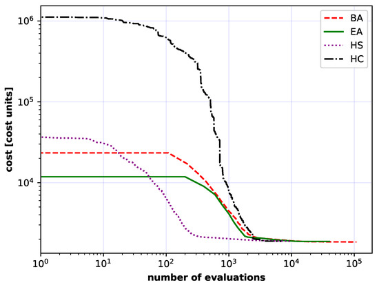
Figure 12. Comparison of the convergence for the USA network of all considered methods: artificial bee colony (BA), evolutionary algorithm (EA), harmony search algorithm (HS) and stochastic hill climbing algorithm (HC). Each curve is an average of 50 independent runs.

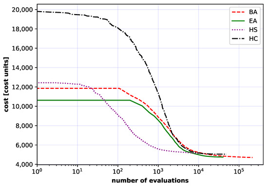
Figure 13. Comparison of the convergence for the American network of all considered methods: artificial bee colony (BA), evolutionary algorithm (EA), harmony search algorithm (HS) and stochastic hill climbing algorithm (HC). Each curve is an average of 50 independent runs.

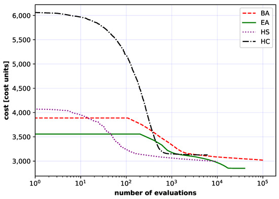
Figure 14. Comparison of the convergence for 50-node the German network of all considered methods: artificial bee colony (BA), evolutionary algorithm (EA), harmony search algorithm (HS) and stochastic hill climbing algorithm (HC). Each curve is an average of 50 independent runs.

It is worth noticing that the ILP approach has one advantage over heuristic methods, i.e., ILP, in that it provides the lower bound for the minimum sought. The results obtained show that for the cases studied ILP is particularly effective when applied to German10, Polish, German15 and German20 networks, since in this case an ILP algorithm finds the optimum. For the USA, American and German networks, as mentioned, ILP finds the lower band and thus allows estimating the optimality gap. However, it is noted that for networks with exceedingly many nodes the optimality gap may be so large as to preclude any practical knowledge concerning the quality of the feasible solutions obtained.

Considering the average results, the HC algorithm performed worst in all cases. On the other hand, the best results in all considered cases for USA, American and German networks were obtained consistently using BA and EA algorithms. BA and EA algorithms both reached the minimum, and most importantly, the lowest average value for the American network. This observation supports the claim that the swarm algorithms (BA and EA) are best suited for optimization of optical networks with a large number of nodes (i.e., USA, American and German). The BA and HC algorithms results have the highest values of the standard deviation. This suggests that BA and HC algorithms explore the solution space more robustly and thus give more diverse results.

In the more complex cases, American, USA and German 50 node networks (Figure 8, Figure 9 and Figure 10), algorithms based mainly on solution space exploitation (HC and HS) converged to a certain point, and then, due to small exploration, stopped at one of the extrema of local solution spaces. At this point, EA and BA algorithms show their superiority. This is because in EA and BA algorithms more emphasis is placed on exploration than in the previous two algorithms (HC and HS), which allows EA and BA algorithms to avoid the trap of local extremes and enables them to continue with further optimization.

The Figure 11, Figure 12, Figure 13 and Figure 14 also show the influence of initialization population by HS, EA and BA algorithms in contrast to HC algorithm. More than one solution at the start gives a potentially better base solution, so that these algorithms find a lower cost solution at the start (the chart starts with a much lower cost value).

Further, it is noted that it took more than 6 days for the IP approach to find a solution, which is still further away from the optimum value than the solutions obtained by heuristic algorithms. On average, it took almost three times less time for the BA algorithm than for IP approach, and almost six times less time was needed by the EA algorithm. This is due to the fact that the iterations of the climbing algorithm are computationally very efficient when compared with other algorithms, e.g., the EA algorithm. Finally, the same amount of time was needed for completing calculations using HS and HC algorithms. In fact, HS and HC algorithms proved to be the fastest among all algorithms tested. However, these algorithms did not find the best solutions, which were provided by BA and EA algorithms.

In the last experiment, fine tuning of the EA was performed. Results concerning tuning of $\mu$ and $\lambda$ parameters are provided, as this emerged as a challenging problem. The purpose of this experiment was to establish best settings for $\mu$ and $\frac{\lambda }{\mu }$. The methodology was as follows: values of $\mu =100$ and $\mu =200$ were set experimentally; then $\frac{\lambda }{\mu }\in \{0.1,0.2,0.5,1,2,5\}$ were tested, $p_c=0.9$ and $p_m=0.05$.

Convergence curves presented in Figure 15, Figure 16, Figure 17 and Figure 18 have similar shapes for different $\frac{\lambda }{\mu }$ values. If $\frac{\lambda }{\mu }$ is small, almost no gain is observed for the first iterations. After the initial iterations, however, quick convergence follows, after which the calculated cost values settle to a constant value. With large $\frac{\lambda }{\mu }$, the initial slow convergence does not occur at all and the fast convergence period is followed again by settling down to a constant value.

Figure 15. Convergence curves (cost vs. iterations) for different combinations of $\mu$ and $\frac{\lambda }{\mu }$ settings. Each curve is an average of 50 independent runs. Values of the $\frac{\lambda }{\mu }$ coefficient are described in the legend of the figure. The results were computed for the Polish network.

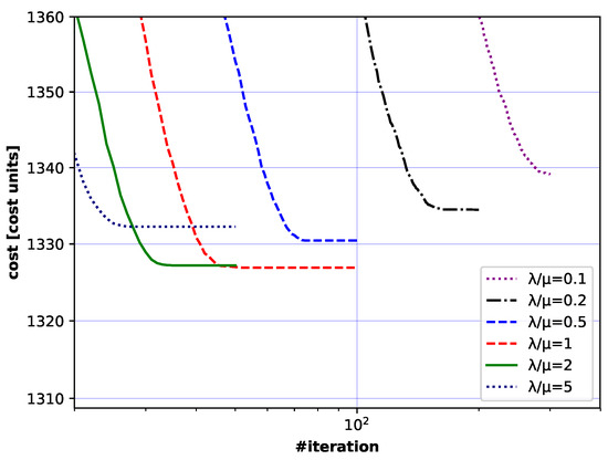
Figure 16. Convergence curves (cost vs. iterations) for different combinations of $\mu$ and $\frac{\lambda }{\mu }$ settings. Zoom of Figure 15.

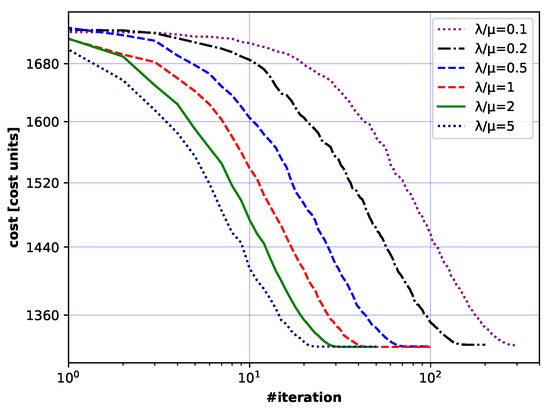
Figure 17. Convergence curves (cost vs. iterations) for different combinations of $\mu$ and $\frac{\lambda }{\mu }$ settings. Each curve is an average of 50 independent runs. Values of the $\frac{\lambda }{\mu }$ coefficient are described in the legend of the figure. The results were computed for the Polish network.

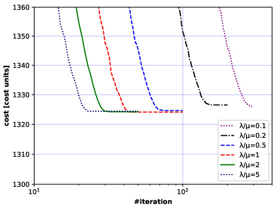
Figure 18. Convergence curves (cost vs. iterations) for different combinations of $\mu$ and $\frac{\lambda }{\mu }$ settings. Zoom of Figure 17.

Thus, the analysis of the impact of the studied parameters on convergence led to the formulation of the following conclusion: if $\mu =100$, $\frac{\lambda }{\mu }$ should be kept to about 1–2 to yield the best EA algorithm performance.

6. Conclusions

To sum up, the following conclusions can be drawn from the analysis for the cases studied. For the German10, Polish, German15 and German20 networks, which are instances of small networks, almost all of the considered methods calculated the optimal solutions. However, for the IP method the calculation time was the lowest for German10 and Polish networks. HS and HC methods can also be successfully used for those cases. However, for the swarm algorithms (BA and EA) calculation times were relatively long. We observed that the EA algorithm is the most efficient for large networks, with the data-sets used in this paper (i.e., USA, American and German), although the BA algorithm was nearly as good.

Finally, it is noted that the results refer to DWDM networks of practical relevance, and hence provide additional guidance for network operators who are planning DWDM network expansions, and since swarm algorithms give promising results when applied to DWDM network optimization, in the near future we plan to continue research on optimizing large networks subject to additional non-linear constraints that are typical for optical networks.

References

- Richardson, D.; Fini, J.; Nelson, L. Space Division Multiplexing in Optical Fibres. Nat. Photonics 2013, 7, 354–362. [Google Scholar] [CrossRef]
- ILOG. CPLEX 11.0 User’s Manual; ILOG: Geneva, Switzerland, 2007. [Google Scholar]
- Garey, M.R.; Johnson, D.S. Computers and Intractability; A Guide to the Theory of NP-Completeness; W. H. Freeman & Co.: New York, NY, USA, 1990. [Google Scholar]
- Klinkowski, M.; Walkowiak, K. Routing and Spectrum Assignment in Spectrum Sliced Elastic Optical Path Network. IEEE Commun. Lett. 2011, 15, 884–886. [Google Scholar] [CrossRef]
- Klinkowski, M.; Żotkiewicz, M.; Walkowiak, K.; Pióro, M.; Ruiz, M.; Velasco, L. Solving large instances of the RSA problem in flexgrid elastic optical networks. IEEE/OSA J. Opt. Commun. Netw. 2016, 8, 320–330. [Google Scholar] [CrossRef]
- Cai, A.; Shen, G.; Peng, L.; Zukerman, M. Novel Node-Arc Model and Multiiteration Heuristics for Static Routing and Spectrum Assignment in Elastic Optical Networks. J. Light. Technol. 2013, 31, 3402–3413. [Google Scholar] [CrossRef]
- Kozdrowski, S.; Żotkiewicz, M.; Sujecki, S. Optimization of Optical Networks Based on CDC-ROADM Technology. Appl. Sci. 2019, 9, 399. [Google Scholar] [CrossRef]
- Żotkiewicz, M.; Ruiz, M.; Klinkowski, M.; Pióro, M.; Velasco, L. Reoptimization of dynamic flexgrid optical networks after link failure repairs. IEEE/OSA J. Opt. Commun. Netw. 2015, 7, 49–61. [Google Scholar] [CrossRef]
- Dallaglio, M.; Giorgetti, A.; Sambo, N.; Velasco, L.; Castoldi, P. Routing, Spectrum, and Transponder Assignment in Elastic Optical Networks. J. Light. Technol. 2015, 33, 4648–4658. [Google Scholar] [CrossRef]
- Kozdrowski, S.; Żotkiewicz, M.; Sujecki, S. Ultra-Wideband WDM Optical Network Optimization. Photonics 2020, 7, 16. [Google Scholar] [CrossRef]
- Shariati, B.; Mastropaolo, A.; Diamantopoulos, N.; Rivas-Moscoso, J.M.; Klonidis, D.; Tomkos, I. Physical-layer-aware performance evaluation of SDM networks based on SMF bundles, MCFs, and FMFs. IEEE/OSA J. Opt. Commun. Netw. 2018, 10, 712–722. [Google Scholar] [CrossRef]
- Poggiolini, P.; Bosco, G.; Carena, A.; Curri, V.; Jiang, Y.; Forghieri, F. The GN-Model of Fiber Non-Linear Propagation and its Applications. J. Light. Technol. 2014, 32, 694–721. [Google Scholar] [CrossRef]
- Yang, X.S. Nature-Inspired Metaheuristic Algorithms; Guide books: Nairobi, Kenya, 2010. [Google Scholar]
- Christodoulopoulos, K.; Tomkos, I.; Varvarigos, E.A. Elastic Bandwidth Allocation in Flexible OFDM-Based Optical Networks. J. Light. Technol. 2011, 29, 1354–1366. [Google Scholar] [CrossRef]
- Syswerda, G. Uniform Crossover in Genetic Algorithms; ICGA’89; Morgan Kaufmann: San Mateo, CA, USA, 1989; pp. 2–9. [Google Scholar] [CrossRef]
- Pham, D.; Ghanbarzadeh, A.; Koç, E.; Otri, S.; Rahim, S.; Zaidi, M. The Bees Algorithm—A Novel Tool for Complex Optimisation Problems. Intell. Prod. Mach. Syst. 2006, 454–459. [Google Scholar] [CrossRef]
- Karaboga, D.; Basturk, B. Artificial Bee Colony (ABC) Optimization Algorithm for Solving Constrained Optimization Problems. In Proceedings of the Foundations of Fuzzy Logic and Soft Computing, 12th International Fuzzy Systems Association World Congress, IFSA 2007, Cancun, Mexico, 18–21 June 2007; Volume 4529, pp. 789–798. [Google Scholar] [CrossRef]
- Yuce, B.; Packianather, M.; Mastrocinque, E.; Pham, D.; Lambiase, A. Honey Bees Inspired Optimization Method: The Bees Algorithm. Insects 2013, 4, 646–662. [Google Scholar] [CrossRef] [PubMed]
- Bäck, H. Proceedings of the Seventh International Conference on Genetic Algorithms: Michigan State University, East Lansing, MI, USA, 19–23 July 1997; Morgan Kaufmann Publishers Inc.: San Francisco, CA, USA, 1997. [Google Scholar]
- Michalkiewicz, Z. Genetic Algorithms + Data Structures = Evolution Programs; Springer: Berlin, Germany, 1996. [Google Scholar]
- Arabas, J.; Kozdrowski, S. Applying an evolutionary algorithm to telecommunication network design. Evol. Comput. IEEE Trans. 2001, 5, 309–322. [Google Scholar] [CrossRef]
- Yang, X.S. Harmony Search as a Metaheuristic Algorithm. 2010. Available online: http://xxx.lanl.gov/abs/1003.1599 (accessed on 20 September 2020).
- Turky, A.M.; Abdullah, S.; McCollum, B.; Sabar, N.R. An Evolutionary Hill Climbing Algorithm for Dynamic Optimisation Problems. In Proceedings of the 6th Multidisciplinary Int. conf. on Scheduling: Theory and Applications (MISTA 2013), Ghent, Belgium, 27–30 August 2013. [Google Scholar]
- Tomlin, J. Branch and Bound Methods for Integer and Nonconvex Programming. In Integer and Nonlinear Programming; Abbie, J., Ed.; North-Holland: Amsterdam, The Netherlands, 1970; pp. 437–450. [Google Scholar]
- Wolsey, L. Integer Programming; John Wiley & Sons: New York, NY, USA, 1998. [Google Scholar]
- Geem, Z.W.; Kim, J.H.; Loganathan, G. A New Heuristic Optimization Algorithm: Harmony Search. SIMULATION 2001, 76, 60–68. [Google Scholar] [CrossRef]
- Beyer, H.G.; Schwefel, H.P. Evolution strategies—A comprehensive introduction. Nat. Comput. 2002, 1, 3–52. [Google Scholar] [CrossRef]
- Arabas, J.; Kozdrowski, S. Population initialization in the context of a biased, problem-specific mutation. In Proceedings of the 1998 IEEE International Conference on Evolutionary Computation Proceedings, IEEE World Congress on Computational Intelligence (Cat. No.98TH8360), Anchorage, AK, USA, 4–9 May 1998; pp. 769–774. [Google Scholar] [CrossRef]
- Orlowski, S.; Wessäly, R.; Pióro, M.; Tomaszewski, A. SNDlib 1.0-Survivable Network Design Library. Networks 2010, 55, 276–286. [Google Scholar] [CrossRef]
© 2020 by the authors. Licensee MDPI, Basel, Switzerland. This article is an open access article distributed under the terms and conditions of the Creative Commons Attribution (CC BY) license (http://creativecommons.org/licenses/by/4.0/).