1. Introduction
Cancer is one of the most fatal and widespread diseases worldwide. Patients can greatly extend their survival time and increase their survival rate with the help of early detection. CT scan is the most commonly used clinical auxiliary method for cancer diagnosis. Physicians make clinical diagnosis on patients through the results of their CT images.However, due to the uneven regional distribution of medical resources, physicians with the abovementioned diagnostic capabilities also show obvious uneven distribution. At the same time, the distribution of cancer patients is relatively random. Therefore, patients in rural areas can only go to central cities for disease diagnosis and treatment, which greatly increases the work intensity of these physicians. However, the complexity of the medical image itself and the high requirements for accuracy of the segmentation result require physicians to perform detailed analysis for a long time. This contradiction has become one of the most urgent problems in cancer diagnosis worldwide. To reduce the workload of physicians and to improve work efficiency, there is a necessity for a high-precision automatic segmentation model to assist physicians in completing medical CT image segmentation tasks [
1].
With the continuous expansion of deep learning applications, convolutional neural network (CNN)-based image semantic segmentation models [
2,
3,
4,
5] have become a better choice to solve the above problems. However, it is not feasible to directly transfer the segmentation model that has been successful in natural image segmentation to the medical image segmentation task because medical images have many characteristics:
High-quality medical image datasets are rare. The special imaging method of medical images produces less data but more false positive phenomena. At the same time, annotating requires countless time, and this process is easily affected by subjective factors such as doctor experience.
Medical images are data with higher dimensions. Compared with the two-dimensional data of natural images, common medical images such as CT and MRI are three-dimensional or higher-dimensional volume data, which is an ordered collection of several two-dimensional images. This makes it impossible to directly read high-dimensional medical image data into the memory, and it is difficult to directly use the natural image segmentation model for training.
The target is smaller in the medical image segmentation, and the boundary of objects is blurred. Compared with objects in natural images, human organs or tumors occupy a very small proportion in medical images, the appearance of the same target under different viewing angles is very different, and the difference between the target and the background is small. The above factors all make the labeling and segmentation of the target extremely difficult.
There is a lack of general pretrained models in this field. The famous ImageNet pretrained model in natural images cannot be transferred to medical image segmentation tasks, and there is insufficient data in medical images to support a pretrained model suitable for most tasks.
It was the fully convolutional neural network proposed by Long [
6] of UC Berkeley and the U-Net proposed by Ronneberger [
7] that brought substantial changes to medical image semantic segmentation. Many researches [
8,
9,
10,
11,
12,
13,
14,
15,
16,
17] were studied based on this work. However, these models usually pay more attention to the overall characteristics of the target, thus ignoring the importance of boundary in medical image segmentation. Such designs are likely to result in a high evaluation indicator, but this high indicator does not represent accurate segmentation of medical images because it does not perform well on boundary segmentation. The rigor of medicine requires higher accuracy of boundaries, especially in human organ image segmentation. Even a small boundary error can lead to misdiagnosis, leading to further work up or unnecessary procedures.
In addition, the occurrence of false positives in the segmentation results can also bring misdiagnosis, leading to deviations in subsequent diagnosis and treatment. For example, the false positive phenomenon in medical segmentation results means that the image segmentation results of the originally healthy patient are positive (ill), which will lead to unnecessary diagnostic procedures and burdens for the patient, and even possibly cause the condition to worsen. However, the above methods did not notice this issue.
To solve the false positive phenomenon mentioned above, we design a classification module for predicting false positive cases. To solve the boundary blur problem mentioned, we adapt a subdivision-based point-sampling method to replace the original upsampling method for “rendering” high-quality boundaries. Besides, we view medical image segmentation as a render problem and propose a network based on 3D U-Net, named Render 3D U-Net, to accurately segment medical 3D CT images. Our contributions in this work conclude the following:
Render 3D U-Net draws on the idea of render in computer graphics and adapts a subdivision-based point-sampling method to replace the original upsampling method for “rendering” high-quality boundaries (
Section 3.2).
Render 3D U-Net integrates the special module (
Section 3.3) into the 3D ANU-Net architecture (
Section 3.1) for classifying a false positive phenomenon.
Render 3D U-Net was evaluated on three public datasets (LiTS, KiTS, and segTHOR) and achieved very competitive performances in three medical image segmentation tasks (
Section 4.4).
Although the render method has been frequently used in computer graphics, to the best of our knowledge, it is the first time that the main idea of render is introduced into a 3D medical image segmentation task.
2. Related Works
2.1. 3D U-Net and Variants
After U-Net [
7] was proposed in 2015 and made extensive research and application in medical image segmentation, lots of U-Net-based variant networks have also proposed, the most representative of which is 3D U-Net [
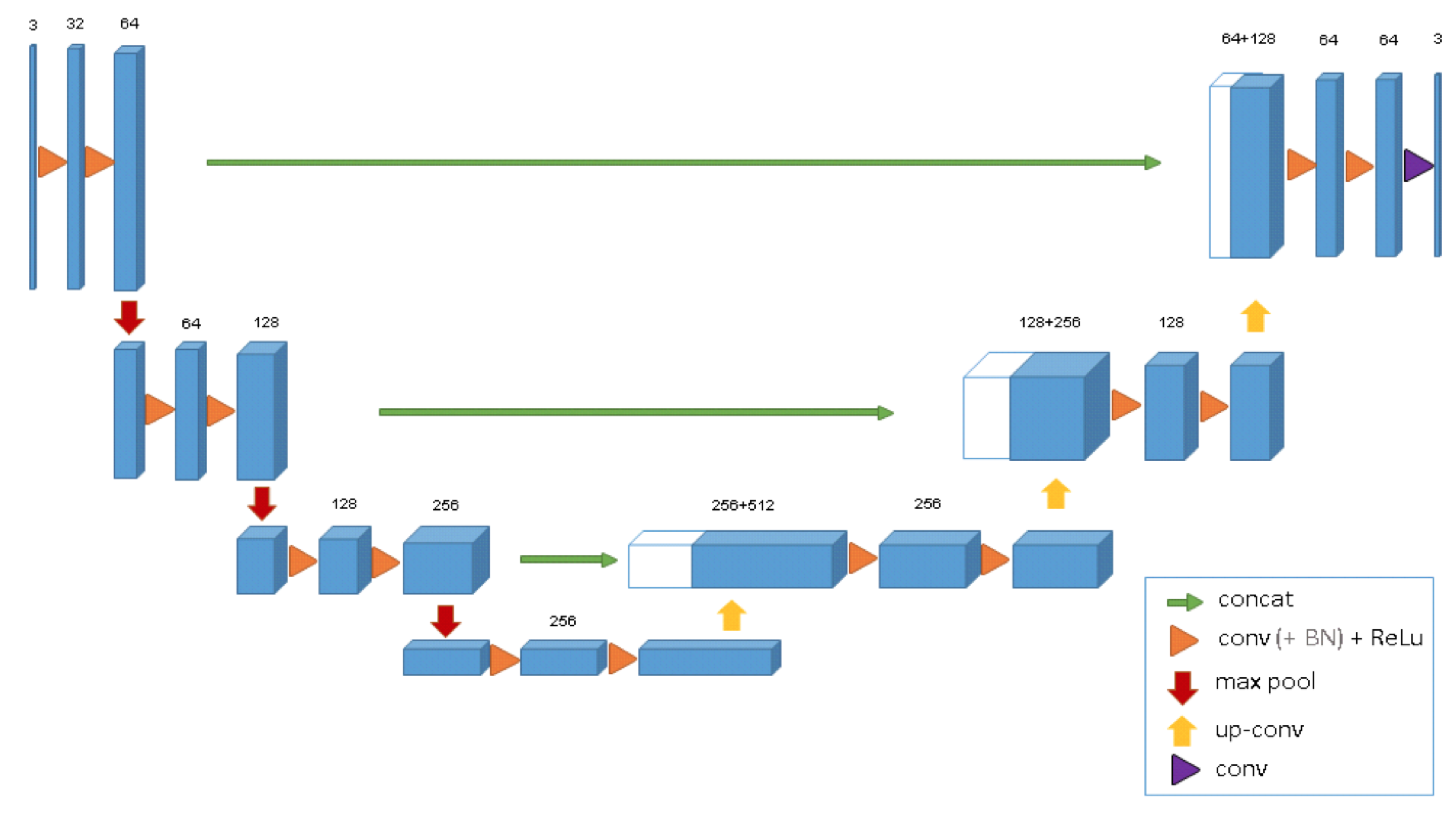
18]. The structure of 3D U-Net is shown in
Figure 1.
This model extends the previous U-Net (2D) and consists of the encoder–decoder architecture. The encoder part analyzes the input image and performs feature extraction and analysis. The corresponding decoder generates a segmented mask. This model supervises the extraction of a mask by minimizing a cost function. What distinguishes 3D U-Net from 2D U-Net is that, after 3D U-Net gets the input of volume data, 3D convolution block, 3D maxpooling, and 3D deconvolution block are used in turn to extract and restore its features. Besides, 3D U-Net adds batch normalization to avoid bottlenecks and to speed up convergence.
Due to its out-performance and simple architecture, 3D U-Net is gradually studied and applied for medical image segmentation tasks [
19,
20,
21,
22]. At the same time, there are also many different variants based on 3D U-Net. nnU-Net [
23] proposed a self-adapting framework based on 2D and 3D vanilla U-Nets. Huang et al. [
24] proposed another 3D U-Net to accurately extract liver vessel from CT images. Zhao et al. [
25] introduced the multi-scale supervision into the decoder and designed postprocessing method to reduce the obviously wrong pixels. Zhou et al. [
26] redesigned skip connections between encoder and decoders to collect features with different scales. Then, they proposed UNet++ for semantic segmentation and instance segmentation.
2.2. Loss Functions for Semantic Segmentation
The loss function is mainly an important indicator used to evaluate the training performance by comparing the similarity between the predicted result and the annotated result. In the field of semantic segmentation, it is very necessary to select an appropriate loss function. In the past few years, there are many loss functions proposed in the existing research, but only a few works [
26] have conducted specific studies on the proposed loss functions. These loss functions can be classified into two types according to different minimization targets.
The first type is distribution-based loss function, in which the goal is to minimize the difference in the distribution of the model output and the real result. The most basic of this category is
cross entropy [
27], and the others are based on cross entropy transformation.
Cross entropy is derived from Kullback–Leibler (KL) divergence [
28] and used to measure the difference between two distributions. For general machine learning tasks, the distribution of data is given by the training set. Therefore, minimizing KL divergence is equivalent to minimizing cross entropy.
Cross entropy (CE) is formulated as follows:
where C represents the number of target labels in the segmentation result. Weighted
cross entropy (WCE) [
29] is a general extended form of cross entropy:
Cross entropy loss performs well in most semantic segmentation tasks, but it encounters difficulties when training with uneven sample distribution. To solve this problem, RetinaNet [
30] proposed focal loss and used the labeled CE to process the uneven distribution of the foreground and background in the image, which can reduce the loss value of the correct classification category. The formulation of
focal loss is:
where the coefficient
was introduced to obtain a better training effect by changing the contribution of the positive and negative samples to the loss.
The another class is area-based loss function, in which the goal is to minimize the mismatched areas between annotated result and model output or to maximize the overlapping area of the annotated result and the model output. The most basic of this category is
dice loss [
31], which is formulated as follows:
The dice loss loss can directly optimize the dice coefficient and is one of the most commonly used segmentation indicators. Unlike cross entropy, it does not need to reweight the unbalanced segmentation tasks.
3. Methodology
In this paper, four methodologies are introduced to reduce the influence of false positive and to solve the boundary blur problem in 3D medical CT image segmentation. The whole overview of these methodologies is described in
Figure 2. Details on the symbols and notation in
Figure 2 are discussed in the next sections.
To collect full spatial information from volume data, Render 3D U-Net is built on the 3D ANU-Net architecture to extract features with rich semantic information (
Section 3.1).
To locate detailed boundary information of the target organ, we propose the point-sampling method to replace the original upsampling method (
Section 3.2).
To reduce the false-positive phenomenon and to achieve more accurate medical image segmentation, we specially designed a module for screening false positive cases and integrated it to the proposed network (
Section 3.3).
To solve the boundary blur problem and to preserve the overall information of target organs at the same time, we integrated the dice loss function and Hausdorff distance into a hybrid loss function (
Section 3.4).
3.1. 3D ANU-Net Architecture
ANU-Net was proposed by Li [
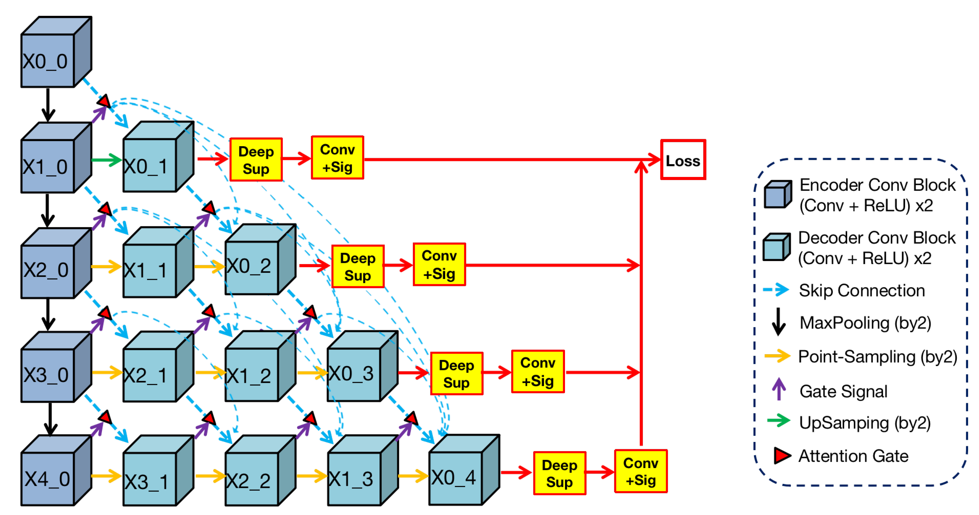
32] and built on UNet++ with an attention mechanism. Render 3D U-Net regarded this work as a basic architecture and changed it to 3D architecture, which is shown in
Figure 3.
We can find from the
Figure 3 that the shape of this architecture is a triangle. In this architecture, the blue convolutional blocks on the left are the shared feature encoder and the remaining green blocks on the right are various decoders. In the encoder, convolutional blocks transfer features through the maxpooling layer from top to bottom. In the decoders, convolution blocks restore the detailed information by
point-sampling the feature from left to right. Between encoder and decoders, semantic information is transferred through dense skip connections under attention selection. Then, the concatenation operation can merge semantic information from different levels, and the fused information is used as the input of every block in the decoder.
3.2. Point-Sampling Method
In the field of image analysis, images are often regarded as regular grids of pixels (points). Their feature vectors are hidden representations on the regular grid of an image. In the task of image semantic segmentation, pixels are upsampled uniformly on the hidden representations and then mapped to a set of labels. These labels will be used as output masks to indicate the predicted category at each pixel. The render method does not calculate labels uniformly on the hidden representation but adaptively selects uncertain points to calculate their labels. We adopt the idea of the classic subdivision [
33] strategy to render high-resolution images from low-resolution features. This strategy only calculates some locations where the values are significantly different from their neighbors. The values at other locations are obtained by interpolating the existing results. This process, named
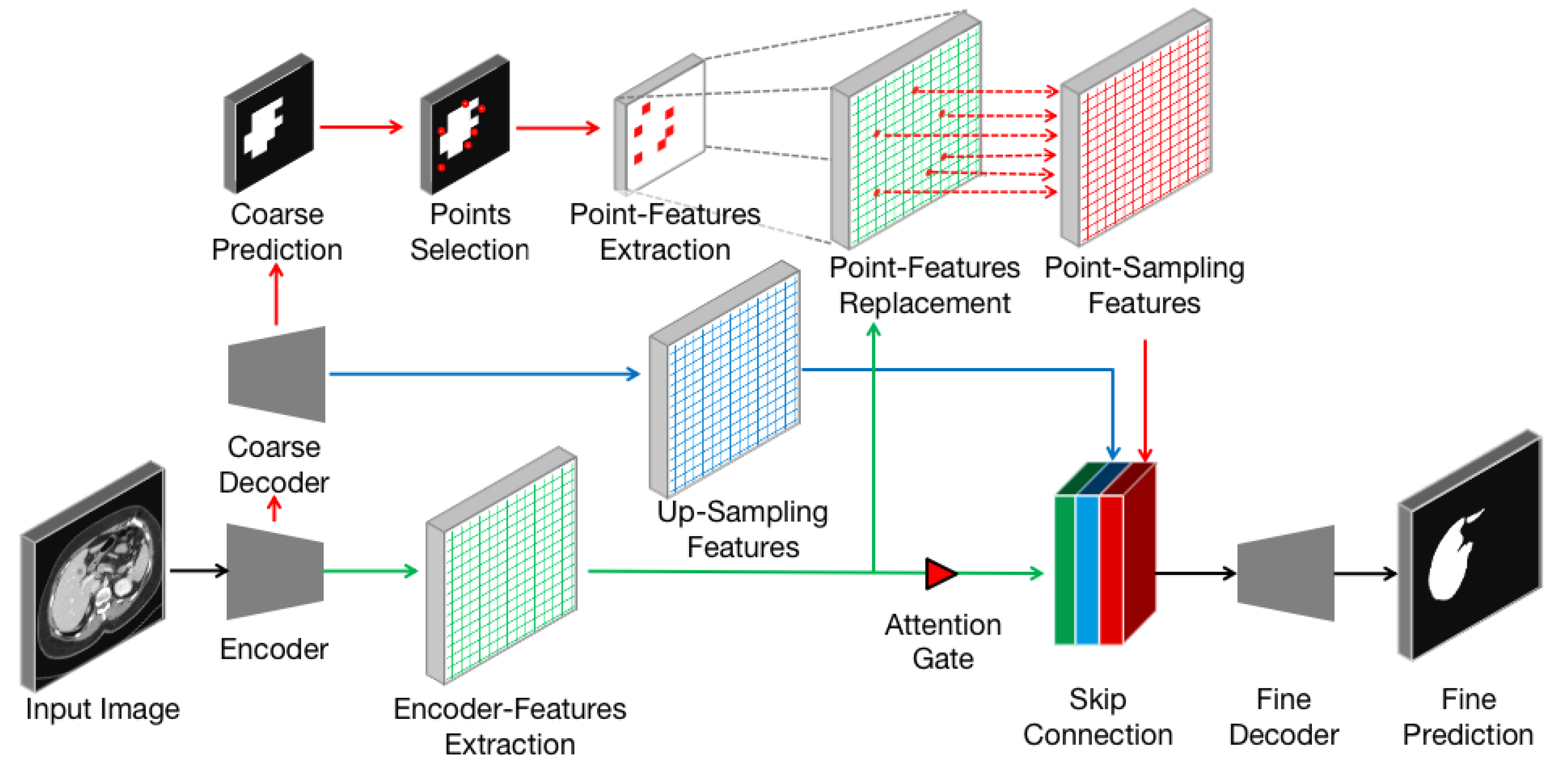
point-sampling method in this paper, restores features from low-resolution by calculating the labels of uncertain points. The point-sampling method is used to replace upsampling method in the 3D ANU-Net architecture and to solve the boundary blur problem. The point-sampling process is described in
Figure 4, which consists of the following steps:
The encoder–decoder architecture (black arrows) takes an input image and extracts features from encoder (green arrows and grids).
The lightweight coarse decoder yields a coarse mask prediction for target object (red arrows) and up-samples features (blue arrows and grids) using bilinear interpolation.
To improve the coarse mask, the point-sampling method selects a set of uncertain points (red dots) from coarse prediction.
A simple multilayer perception is used to extract the point-features of each point independently and predicts their labels.
The point features are mapped to the size of the encoder feature (dashed gray arrows), and the features at the corresponding position are replaced (dashed red arrows) to obtain the point-sampling features (red grids).
The encoder features are concatenated with the up-sampling feature and point-sampling features after passing through the attention gate.
The concatenated features are input into the fine decoder (black arrows) to obtain the fine prediction result.
Compared with the original up-sampling method, the point-sampling method increases the selection of uncertain points (step 3) and the extraction of point features (step 4). Therefore, how to flexibly and adaptively select uncertain points in the image and to extract corresponding point features to enhance segmentation has become the key of the proposed method.
Point selection strategy: The main idea of our selection strategy is that uncertain points are also difficult to classify and belongs to the middle area in the probability distribution. After the coarse mask was predicted by a coarse decoder, there are N most uncertain points on the image plane. We believe that the selection of the most uncertain points should not only focus on uncertain areas (e.g., the boundaries between different classes) but also should retain a certain degree of uniform coverage. Such a design can achieve the greatest degree of accurate segmentation and can enhance anti-interference abilities.
To achieve the goal, we referred to the following principles in [
34] for point selection and balance. In this way, we obtained the fine predicted mask from low resolution.
Overgeneration: first, randomly sample KN points from a uniformlydistributed point set. These KN will be used to overgenerate candidate points, and k should be greater than 1.
Important sampling: then, we will coarsely predict the segmentation class of the above KN and then perform interpolation, calculate the uncertainty estimation of all points on the segmentation task, and select the top N points with the highest uncertainty. These points are considered important points.
Unimportant sampling: after removing the abovementioned important points from KN, ()N points remain. These points are regarded as unimportant points sampled from a uniform distribution.
3.3. False-Positives Classification Module (FPC)
Clinically, positive represents abnormal tissue or some disease in the human body and negative represents normal. False positive refers to a phenomenon in which one healthy (negative) person receives a positive symptom. In short, it is a disease-free misdiagnosis. False positives are common in medical detection. Since there are more pure negative samples in medical image data, the imbalance between positive and negative data is serious. Therefore, in most medical image organ segmentation tasks, false positive results (organs detected in no-organ images) are frequent occurrences. False positive results may lead to more serious follow-up medical accidents, resulting in a waste of hospital medical resources and psychological distress to the patient, thereby causing physical and mental harm to patients.
In order to solve this problem and to achieve more accurate medical image segmentation, we specially designed a module (FPC) for screening false positive phenomena and added it to the proposed network model. Our goal is to determine whether there is an organ in the input image through this module and to predict the mask based on the screening results.
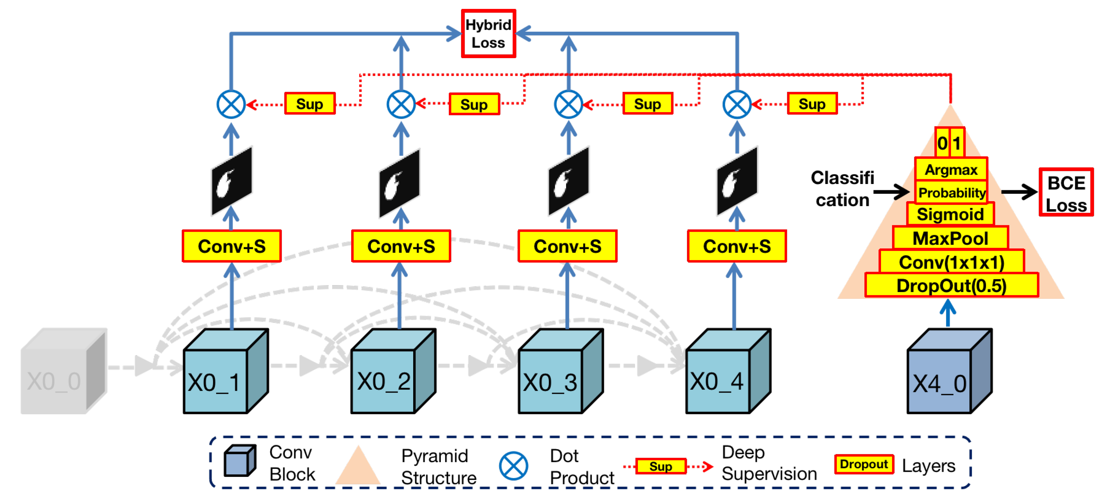
The architecture of FPC is shown in
Figure 5. In the Render3D U-Net architecture, the deepest block (
) in the encoder owns the richest semantic information after hierarchical convolution operations. To make full use of it, we designed a pyramid structure to extract organ existence information in semantic features. This pyramid structure is composed of the following layers from bottom to top:
Dropout layer (by 0.5): this layer can effectively prevent the network training from overfitting.
Convolution layer and adaptive maxpool layer (by 2): these two layers can extract organ features from semantic information.
Sigmoid layer (): this layer is a mathematical tool that can obtain the probability value of binary classification (), which represents the uncertainty of the organ existence in the input image.
Argmax layer: this layer can select the highest probability value among , where 0 represents no existence of an organ and 1 represents the existence of an organ.
Then, the FPC module dot products of the output image from the nodes in the first layer with the classification results or :
If the previous step determines that there is an organ in the input image, the result of the dot product with 1 will still be the original output.
Otherwise, the result of the dot product with 0 will be black, thereby reducing the possibility of misdiagnosis as a false positive.
In essence, the FPC module is a binary classification task and then blackens the output mask of nonexistent organs according to the classification result. In order to train this module, we take advantage of the simplicity of the binary classification task and used binary cross entropy (BCE) as the loss function. This loss can help reduce the possibility of oversegmentation caused by false positives while preserving the original organ features to the greatest extent. Eventually, the impact of false positives is reduced by the false positive classification module.
3.4. Hybrid Loss Function
To solve the boundary blur problem but to preserve the overall information of the target organ, Render 3D U-Net adds deep supervision [
32] with ground truth after every output block (
) and connects these blocks directly to loss function for calculating the sum loss. Besides, we integrate two loss functions into a hybrid loss function, including dice loss and Hausdorff distance. Formulation of this
hybrid loss function is as follows:
where
is the output of block
and
is the ground truth,
s is the smooth soft dice coefficient part, and ∘ is the operation of the Hadamard product,
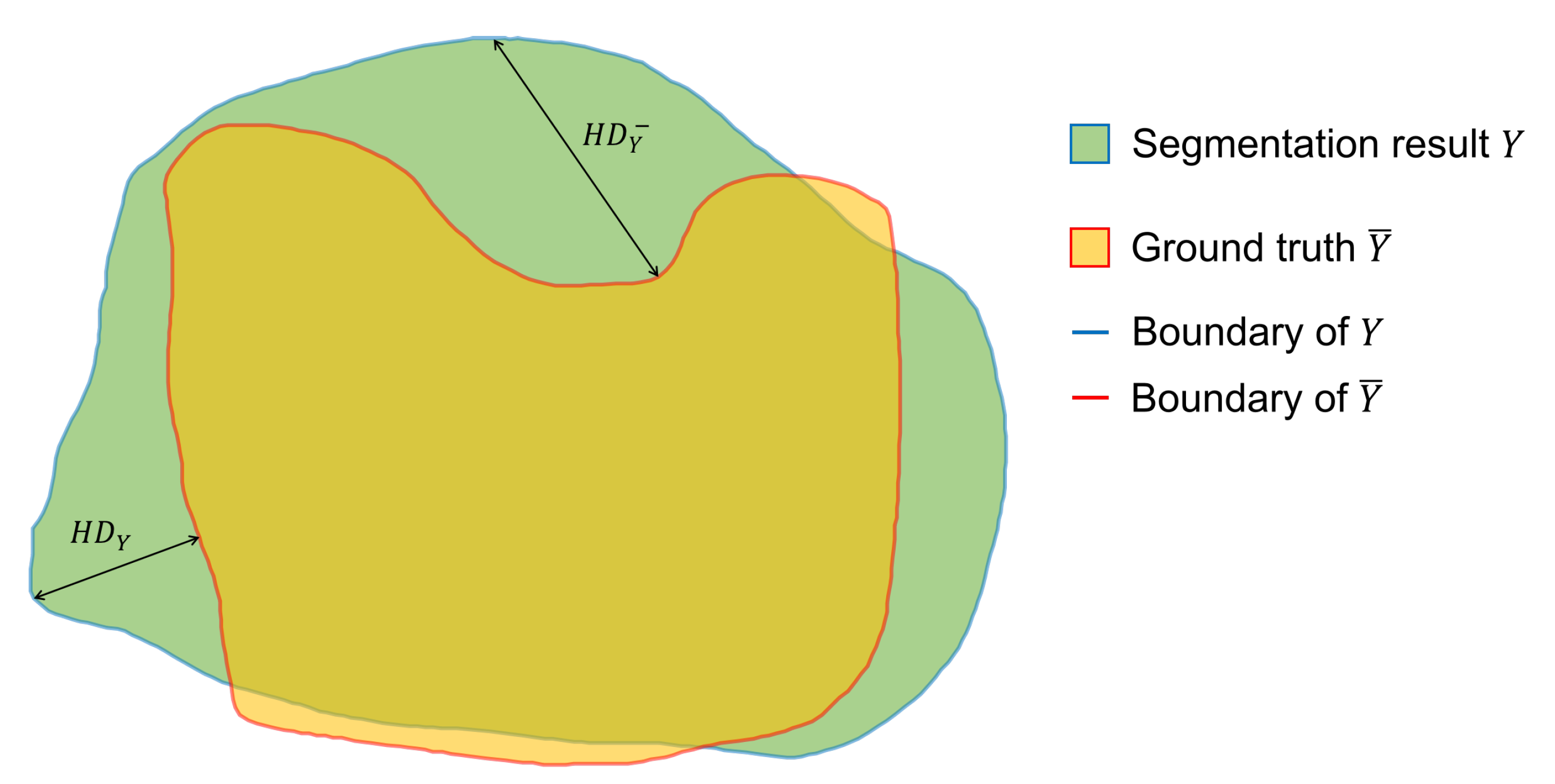
denotes the Hausdorff distance between the boundaries of predicted result and annotated result. The Hausdorff distance (
HD) is defined as follows and the diagram of Hausdorff distance is shown in
Figure 6:
where
is the Euclidean distance and
.
As we can see,
is the soft Dice coefficient. This index represents the area of overlap between the model output and the annotated result. This index can help the model pay attention to the overall information of the target organ, but it cannot effectively supervise the boundary contour. As a consequence, we referred to the research by [
35] and introduced the Hausdorff distance for strengthening the learning of boundaries and to solve the boundary blur problem.
measures the segmentation performance on boundary by calculating the Hausdorff distance between the model output boundary and the ground truth boundary.
4. Experiments And Results
We designed four experiments (segmentation experiment, attention learning experiment, point-sampling experiment, and false-positive classification experiment) to prove our improvement due to the introduced methodologies.
4.1. Dataset Introduction
The above four experiments are all based on public medical image datasets, covering common organs from medical imaging modality. The detailed information is shown in the
Table 1.
The LiTS [
36] dataset is from the Liver Tumor Segmentation Challenge, which was held in MICCAI 2017. The training set of this dataset has 130 CT volumes, and the test set has 70 CT volumes. There are three types of objects in the LiTS dataset: liver, tumor, and background. In this segmentation experiment, we only focus on the liver and regard it as a positive object and the others as a negative object.
The KiTS [
37] dataset is from the Kidney and Kidney Tumor Segmentation Challenge in MICCAI 2019. The training set has 210 CT volumes, and the test set has 90 CT volumes. Similarly, there are three types of objects in the KiTS dataset: kidney, tumor, and background. In this segmentation experiment, we only focus on the kidney and regard it as a positive object and the others as a negative object
The SegTHOR [
38] dataset is from the Segmentation of THoracic Organs at Risk in CT images challenge in ISBI 2019. The training set has 40 CT volumes, and the test set has 20 CT volumes. There are four types of objects in the SegTHOR dataset: heart, aorta, trachea, and esophagus. In this segmentation experiment, we only focus on the heart and regard it as a positive object and the others as a negative object.
Since the data shape (length, width, and thickness of the volume) of the three datasets are different, we unified the data into a patch of 256 × 256 × 32 size. Finally, we used the training set in the above three datasets as the data for this experiment and then divided it into the training set and test set at a ratio of 5:1.
4.2. Performance Evaluation
We used four popular indicators in medical image segmentation tasks to evaluate organ segmentation quality, including IoU [
18], dice [
31] and recall [
39]. In addition, we also use Hausdorff distance (HD) [
35] as an indicator to measure the performance of boundary segmentation. The above metrics are formulated as follows:
where
and
are the true positive, true negative, false positive, and false negative respectively.
Y means the segmentation result when
is the annotated result.
means thecalculation of the Manhattan distance. As the values of the first four indicators rise, the similarity increases and the accuracy of segmentation improves. The Hausdorff distance is added for evaluation of the segmentation on boundary.
4.3. Feature Visualization
In
Section 3.1 and
Section 3.4, we introduced the 3D nested convolution structure and dense skip connection in Render 3D U-Net. In this section, we visually displayed the features of the output layer, which more intuitively confirms the superiority of the network structure for semantic feature extraction.
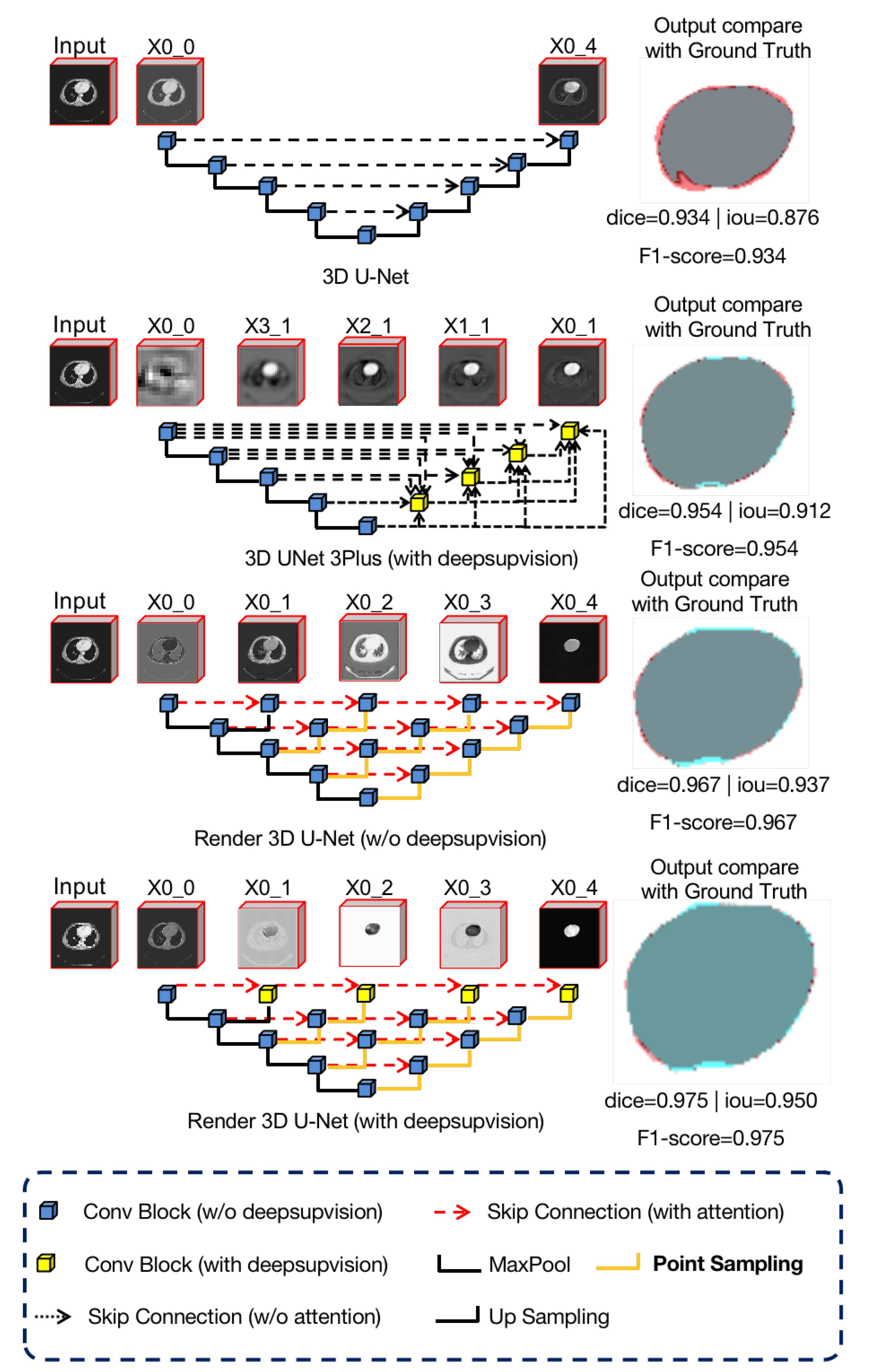
As we can see in
Figure 7, we used four different networks for the liver CT images segmentation task and visualized the features of the output layer
. These four networks included 3D U-Net [
7], 3D UNet3+ [
40], Render 3D U-Net without deep supervision, and Render 3D U-Net with deep subdivision.
We observe that the feature representation of U-Net is not clear enough and that the complete semantic information is not extracted. This is because the original skip connection in U-Net is relatively simple and the lower layer features are directly connected to the encoder features after upsampling. In comparison, the features in UNet++ and Render 3D U-Net are connected by more complex skip connections, which merge more semantic information and gradually form a clearer feature representation. In addition, we can also observe that, due to the introduction of hybrid loss (
Section 3.4), the loss of each output node can be calculated, which helps Render 3D U-Net to extract semantic information better.
4.4. Segmentation Results
Render 3D U-Net competes against the other seven popular models (3D UNet [
18], 3D R2UNet [
41], 3D UNet++ [
42], Attention 3D UNet [
43], Attention 3D R2UNet, and 3D UNet3+ [
40]) on medical CT image segmentation tasks. Besides, we combine the proposed point-sampling method with UNet++ and added this Point UNet++ to the comparison. The experiments results are summarized in the following table, where DS means deep supervision, HD means Hausdorff distance. Note that the prediction time is the mean time it takes to predict each 3D volume in the test dataset. The GPU used in the test is a single NVIDIA GeForce GTX 1080TI.
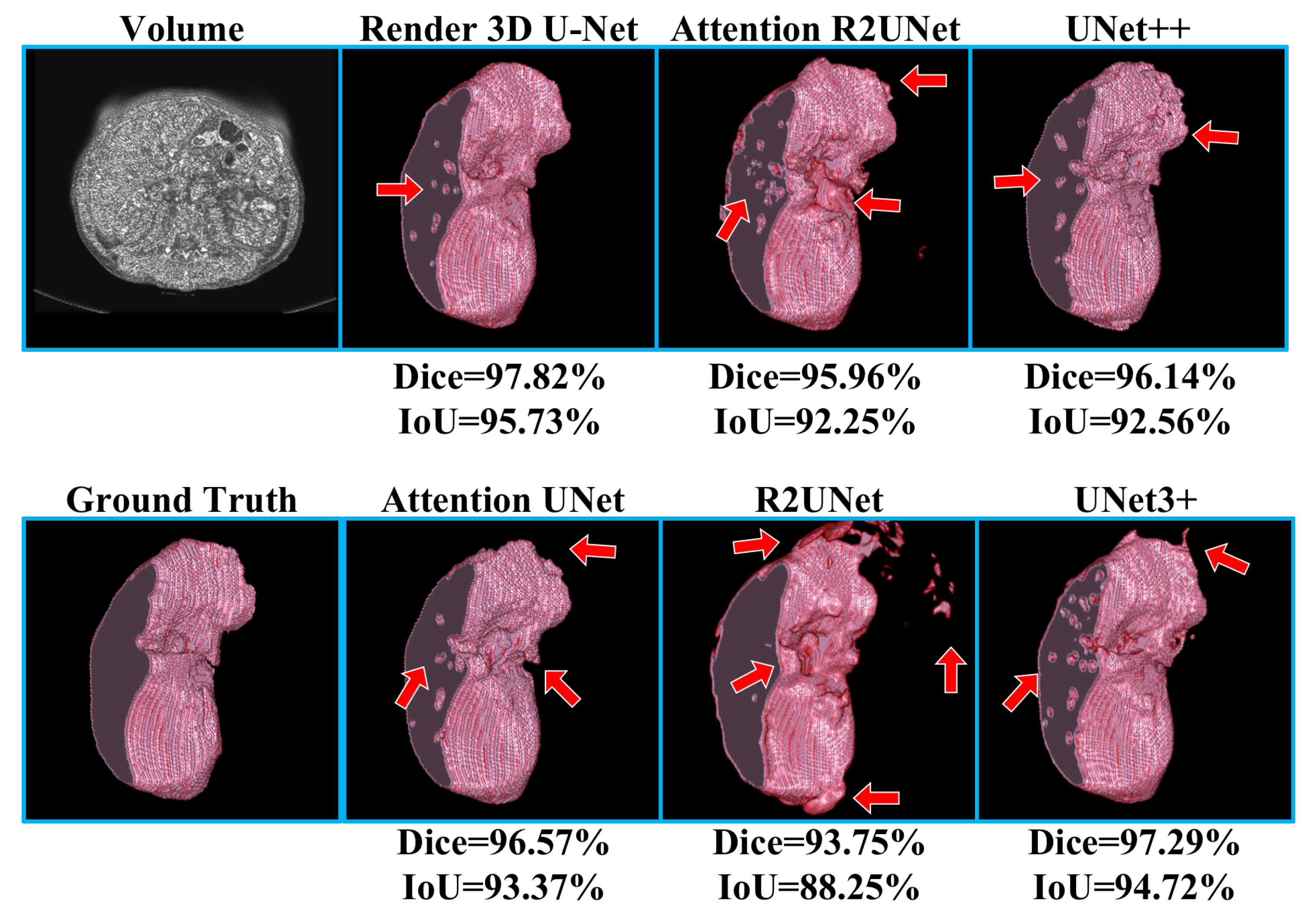
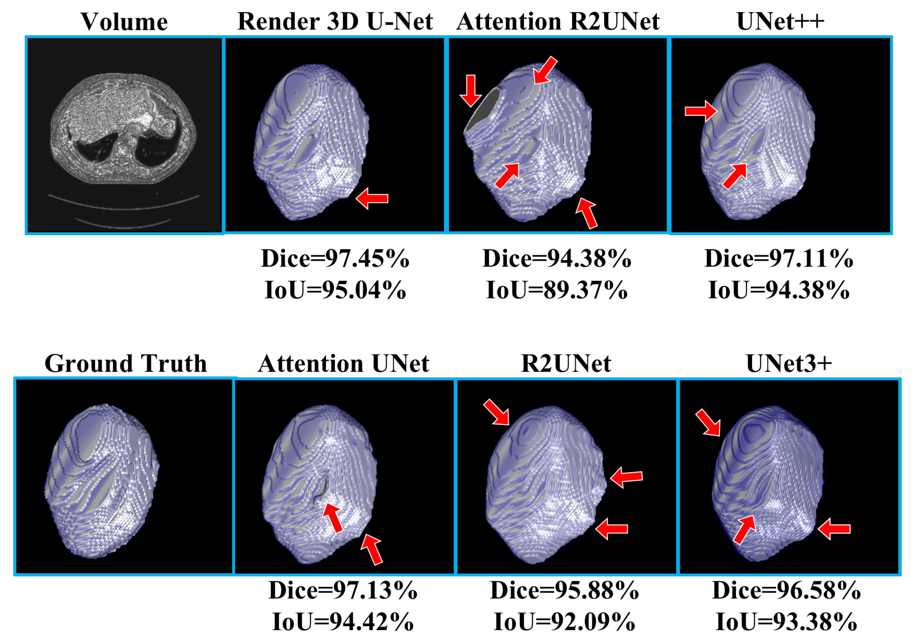
Table 2 shows the experimental results of liver CT volume segmentation, the performance of Render 3D U-Net is the best. We can get the conclusion that the introduction of FPC can help the network obtain a better performance on liver CT volume segmentation. The output of the model and the manually annotated result are compared in
Figure 8. Render 3D U-Net increased the IoU ratio by 2.85 percentage points over Attention 3D UNet, increased the dice coefficient by 1.62 percentage points, increased the recall rate by 0.0269, and decreased the Hausdorff distance by 3.6357.
Table 3 shows the experimental results of kidney CT volume segmentation; the performance of Render 3D U-Net is the best. We can get the conclusion that the introduction of FPC can help the network obtain a better performance on kidney CT volume segmentation. The output of the model and the manually annotated result are compared in
Figure 9. Render 3D U-Net increased the IoU ratio by 5.12 percentage points over 3D UNet3+, increased the dice coefficient by 3.06 percentage points, increased the recall rate by 0.0333, and decreased the Hausdorff distance by 1.0914.
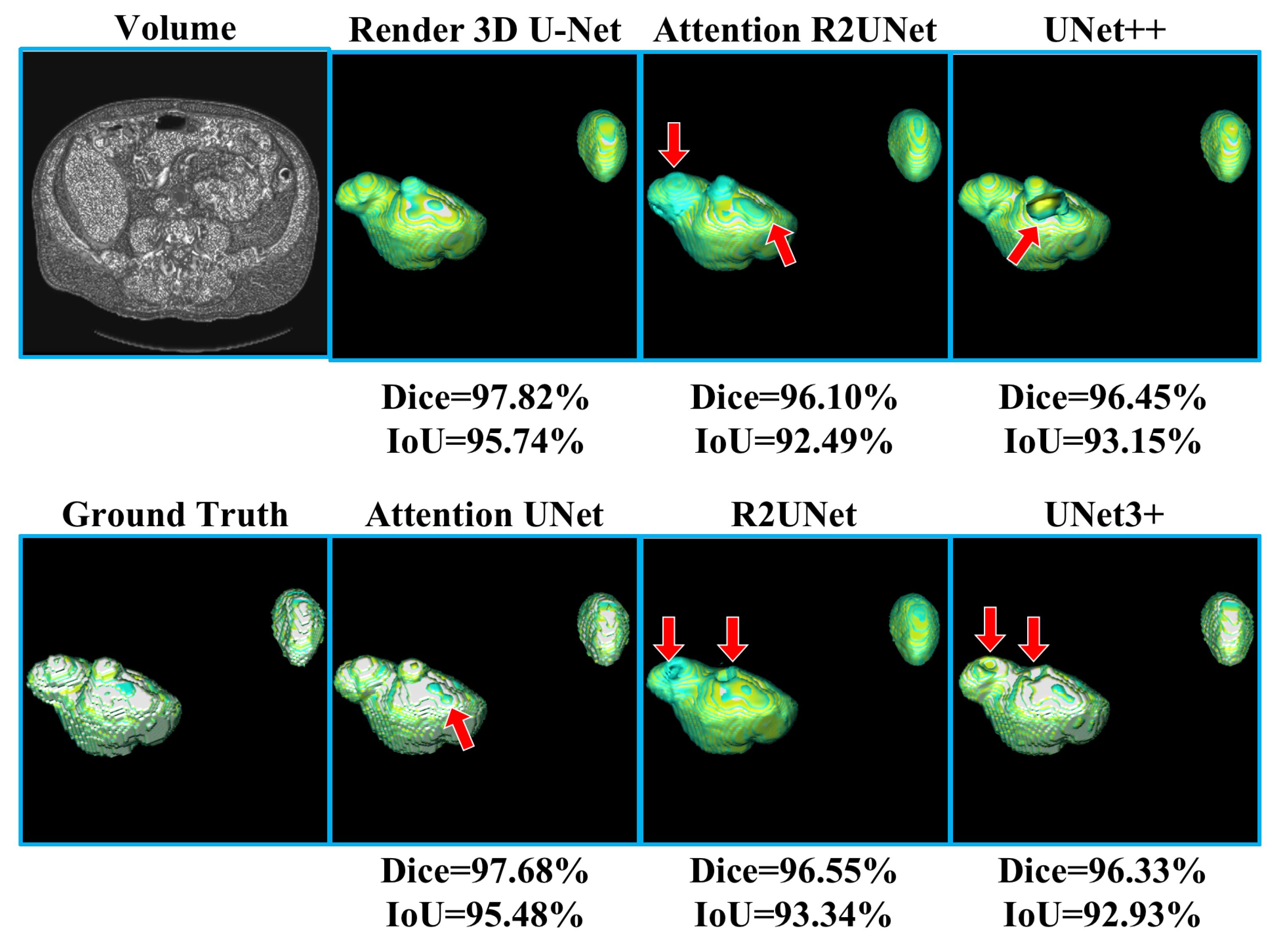
Table 4 shows the experimental results of heart CT volume segmentation; the performance of Render 3D U-Net is the best. We can get the conclusion that the introduction of FPC can help network obtain a better performance on heart CT volume segmentation. The output of model and the manually annotated result are compared in
Figure 10. Render 3D U-Net increased the IoU ratio by 4.17 percentage points over Attention 3D R2UNet, increased the dice coefficient by 2.34 percentage points, increased the recall rate by 0.0223, and decreased the Hausdorff distance by 1.8036.
It is obvious that the proposed network outperformed other networks in the above three segmentation tasks. The comparison between Point UNet++ and UNet++ without point-sampling method proved that the introduction of point-sampling method can help Point UNet++ always perform better than UNet++. These comparisons strongly prove that the improvement is attributed to the proposed point-sampling method and false positive classification module.
4.5. False Positive Classification Results
According to the results from
Table 2 through
Table 4, it is obvious that, after introduction of the False Positive Classification (FPC) module, Render 3D U-Net decreases the false positive phenomena and improves performance on medical volume segmentation. In the liver segmentation task, the FPC module helped Render 3D U-Net obtain a better performance on mIoU and dice. In the kidney segmentation task, Render 3D U-Net with the FPC module obtained a higher mIoU and dice. In the heart segmentation task, Render 3D U-Net with the FPC module obtained a higher mIoU and Dice. Another comparison between Render 3D U-Net with FPC and Render 3D U-Net without FPC also confirmed the effectiveness of proposed FPC module in solving false positive phenomena and in improving performance. These comparisons strongly prove again that the improvement is attributed to the proposed point-sampling method and false positive classification module.
5. Conclusions
In this paper, we provided a unique perspective on render and viewed the 3D medical CT image segmentation task as a render problem. We adapted a subdivision-based point-sampling method to replace the original upsampling method for “rendering” high-quality boundaries. Besides, we designed a false positive classification module for reducing the influence of false positive phenomena. We integrated the above methods into 3D ANU-Net and competed with other seven popular models on organ segmentation tasks. The experiments on the three public datasets proved that the proposed model successfully solves the boundary blur problem and reduces the influence of false positive phenomena. We believe that the improvement is attributed to the introduction of the point-sampling method and false positive classification (FPC) module. The point-sampling method has been proven to render higher quality boundaries than traditional upsampling method. The FPC module has been proven to reduce the influence caused by false positive phenomena and to improve the segmentation performance at the same time.
Author Contributions
C.L.: methodology and writing—original draft; W.C.: methodology, supervision, and writing—review and editing; Y.T.: project administration. All authors have read and agreed to the published version of the manuscript.
Funding
This work was supported by the National Key Research and Development Program of China (No. 2018YFB0204301).
Conflicts of Interest
The authors declare no conflict of interest.
References
- Mei, X.; Lee, H.C.; Diao, K.Y.; Huang, M.; Lin, B.; Liu, C.; Xie, Z.; Ma, Y.; Robson, P.; Chung, M.; et al. Artificial intelligence-enabled rapid diagnosis of patients with COVID-19. Nat. Med. 2020, 26, 1224–1228. [Google Scholar] [CrossRef]
- Badrinarayanan, V.; Kendall, A.; Cipolla, R. Segnet: A deep convolutional encoder-decoder architecture for image segmentation. IEEE Trans. Pattern Anal. Mach. Intell. 2017, 39, 2481–2495. [Google Scholar] [CrossRef]
- Chen, L.C.; Papandreou, G.; Kokkinos, I.; Murphy, K.; Yuille, A.L. Deeplab: Semantic image segmentation with deep convolutional nets, atrous convolution, and fully connected crfs. IEEE Trans. Pattern Anal. Mach. Intell. 2017, 40, 834–848. [Google Scholar] [CrossRef]
- Papandreou, G.; Chen, L.C.; Murphy, K.P.; Yuille, A.L. Weakly-and semi-supervised learning of a deep convolutional network for semantic image segmentation. In Proceedings of the IEEE International Conference on Computer Vision, Santiago, Chile, 7–13 December 2015; pp. 1742–1750. [Google Scholar]
- Lin, G.; Shen, C.; Van Den Hengel, A.; Reid, I. Efficient piecewise training of deep structured models for semantic segmentation. In Proceedings of the IEEE Conference on Computer Vision and Pattern Recognition, Las Vegas, NV, USA, 27–20 June 2016; pp. 3194–3203. [Google Scholar]
- Long, J.; Shelhamer, E.; Darrell, T. Fully Convolutional Networks for Semantic Segmentation. IEEE Trans. Pattern Anal. Mach. Intell. 2014, 39, 640–651. [Google Scholar]
- Ronneberger, O.; Fischer, P.; Brox, T. U-net: Convolutional networks for biomedical image segmentation. In Proceedings of the International Conference on Medical Image Computing and Computer-Assisted Intervention, Munich, Germany, 5–9 October 2015; Springer: Berlin, Germany, 2015; pp. 234–241. [Google Scholar]
- Dolz, J.; Gopinath, K.; Yuan, J.; Lombaert, H.; Desrosiers, C.; Ayed, I.B. HyperDense-Net: A hyper-densely connected CNN for multi-modal image segmentation. IEEE Trans. Med. Imaging 2018, 38, 1116–1126. [Google Scholar] [CrossRef] [PubMed]
- Moeskops, P.; Wolterink, J.M.; van der Velden, B.H.; Gilhuijs, K.G.; Leiner, T.; Viergever, M.A.; Išgum, I. Deep learning for multi-task medical image segmentation in multiple modalities. In Proceedings of the International Conference on Medical Image Computing and Computer-Assisted Intervention, Athens, Greece, 17–21 October 2016; Springer: Cham, Switzerland, 2016; pp. 478–486. [Google Scholar]
- Oktay, O.; Ferrante, E.; Kamnitsas, K.; Heinrich, M.; Bai, W.; Caballero, J.; Cook, S.A.; De Marvao, A.; Dawes, T.; O‘Regan, D.P.; et al. Anatomically constrained neural networks (ACNNs): Application to cardiac image enhancement and segmentation. IEEE Trans. Med. Imaging 2017, 37, 384–395. [Google Scholar] [CrossRef] [PubMed]
- Kamnitsas, K.; Ledig, C.; Newcombe, V.F.; Simpson, J.P.; Kane, A.D.; Menon, D.K.; Rueckert, D.; Glocker, B. Efficient multi-scale 3D CNN with fully connected CRF for accurate brain lesion segmentation. Med. Image Anal. 2017, 36, 61–78. [Google Scholar] [CrossRef] [PubMed]
- Zhang, W.; Li, R.; Deng, H.; Wang, L.; Lin, W.; Ji, S.; Shen, D. Deep convolutional neural networks for multi-modality isointense infant brain image segmentation. NeuroImage 2015, 108, 214–224. [Google Scholar] [CrossRef] [PubMed]
- Drozdzal, M.; Vorontsov, E.; Chartrand, G.; Kadoury, S.; Pal, C. The importance of skip connections in biomedical image segmentation. In Deep Learning and Data Labeling for Medical Applications; Springer: Cham, Switzerland, 2016; pp. 179–187. [Google Scholar]
- Havaei, M.; Davy, A.; Warde-Farley, D.; Biard, A.; Courville, A.; Bengio, Y.; Pal, C.; Jodoin, P.M.; Larochelle, H. Brain tumor segmentation with deep neural networks. Med. Image Anal. 2017, 35, 18–31. [Google Scholar] [CrossRef] [PubMed]
- Li, X.; Chen, H.; Qi, X.; Dou, Q.; Fu, C.W.; Heng, P.A. H-DenseUNet: Hybrid densely connected UNet for liver and tumor segmentation from CT volumes. IEEE Trans. Med. Imaging 2018, 37, 2663–2674. [Google Scholar] [CrossRef]
- Payer, C.; Štern, D.; Bischof, H.; Urschler, M. Multi-label whole heart segmentation using CNNs and anatomical label configurations. In Proceedings of the International Workshop on Statistical Atlases and Computational Models of the Heart, Quebec City, QC, Canada, 10–14 September 2017; Springer: Cham, Switzerland, 2017; pp. 190–198. [Google Scholar]
- Liao, F.; Liang, M.; Li, Z.; Hu, X.; Song, S. Evaluate the Malignancy of Pulmonary Nodules Using the 3-D Deep Leaky Noisy-or Network. IEEE Trans. Neural Netw. Learn. Syst. 2019, 30, 3484–3495. [Google Scholar] [CrossRef]
- Çiçek, Ö.; Abdulkadir, A.; Lienkamp, S.S.; Brox, T.; Ronneberger, O. 3D U-Net: Learning dense volumetric segmentation from sparse annotation. In Proceedings of the International Conference on Medical Image Computing And Computer-Assisted Intervention, Athens, Greece, 17–21 October 2016; Springer: Cham, Switzerland, 2016; pp. 424–432. [Google Scholar]
- Beers, A.; Chang, K.; Brown, J.M.; Sartor, E.; Mammen, C.P.; Gerstner, E.R.; Rosen, B.R.; Kalpathycramer, J. Sequential 3D U-Nets for Biologically-Informed Brain Tumor Segmentation. arXiv 2017, arXiv:1709.02967. [Google Scholar]
- Kakeya, H.; Okada, T.; Oshiro, Y. 3D U-JAPA-Net: Mixture of Convolutional Networks for Abdominal Multi-organ CT Segmentation. In Medical Image Computing and Computer Assisted Intervention—MICCAI 2018; Springer: Cham, Switzerland, 2018; pp. 426–433. [Google Scholar]
- Hwang, H.; Rehman, H.Z.U.; Lee, S. 3D U-Net for Skull Stripping in Brain MRI. Appl. Sci. 2019, 9, 569. [Google Scholar] [CrossRef]
- Huang, C.; Han, H.; Yao, Q.; Zhu, S.; Zhou, S.K. 3D U2-Net: A 3D Universal U-Net for Multi-Domain Medical Image Segmentation. arXiv 2019, arXiv:1909.06012. [Google Scholar]
- Isensee, F.; Petersen, J.; Klein, A.; Zimmerer, D.; Jaeger, P.F.; Kohl, S.; Wasserthal, J.; Koehler, G.; Norajitra, T.; Wirkert, S.J.; et al. nnU-Net: Self-adapting Framework for U-Net-Based Medical Image Segmentation. arXiv 2018, arXiv:1809.10486. [Google Scholar]
- Huang, Q.; Sun, J.; Ding, H.; Wang, X.; Wang, G. Robust liver vessel extraction using 3D U-Net with variant dice loss function. Comput. Biol. Med. 2018, 101, 153–162. [Google Scholar] [CrossRef]
- Zhao, W.; Zeng, Z. Multi Scale Supervised 3D U-Net for Kidney and Tumor Segmentation. arXiv 2019, arXiv:1908.03204. [Google Scholar]
- Zhou, Z.; Siddiquee, M.M.R.; Tajbakhsh, N.; Liang, J. UNet++: Redesigning Skip Connections to Exploit Multiscale Features in Image Segmentation. IEEE Trans. Med. Imaging 2019. [Google Scholar] [CrossRef]
- Byrne, C. Iterative image reconstruction algorithms based on cross-entropy minimization. IEEE Trans. Image Process. 1993, 2, 96–103. [Google Scholar] [CrossRef]
- Rubinstein, R.Y. The Cross-Entropy Method for Combinatorial and Continuous Optimization. Methodol. Comput. Appl. Probab. 1999, 1, 127–190. [Google Scholar] [CrossRef]
- Bertels, J.; Eelbode, T.; Berman, M.; Vandermeulen, D.; Maes, F.; Bisschops, R.; Blaschko, M.B. Optimizing the Dice score and Jaccard index for medical image segmentation: Theory and practice. In Proceedings of the International Conference on Medical Image Computing and Computer-Assisted Intervention, Shenzhen, China, 13–17 October 2019; Springer: Cham, Switzerland, 2019; pp. 92–100. [Google Scholar]
- Lin, T.Y.; Goyal, P.; Girshick, R.; He, K.; Dollár, P. Focal loss for dense object detection. In Proceedings of the IEEE International Conference on Computer Vision, Venice, Italy, 22–29 October 2017; pp. 2980–2988. [Google Scholar]
- Menze, B.H.; Jakab, A.; Bauer, S.; Kalpathycramer, J.; Farahani, K.; Kirby, J.; Burren, Y.; Porz, N.; Slotboom, J.; Wiest, R.; et al. The Multimodal Brain Tumor Image Segmentation Benchmark (BRATS). IEEE Trans. Med. Imaging 2015, 34, 1993–2024. [Google Scholar] [CrossRef] [PubMed]
- Li, C.; Tan, Y.; Chen, W.; Luo, X.; He, Y.; Gao, Y.; Li, F. ANU-Net: Attention-based Nested U-Net to exploit full resolution features for medical image segmentation. Comput. Graph. 2020, 90, 11–20. [Google Scholar] [CrossRef]
- Whitted, T. An Improved Illumination Model for Shaded Display. SIGGRAPH Comput. Graph. 1979, 13, 14. [Google Scholar] [CrossRef]
- Kirillov, A.; Wu, Y.; He, K.; Girshick, R. PointRend: Image Segmentation as Rendering. arXiv 2019, arXiv:1912.08193. [Google Scholar]
- Karimi, D.; Salcudean, S.E. Reducing the Hausdorff Distance in Medical Image Segmentation with Convolutional Neural Networks. IEEE Trans. Med. Imaging 2020, 39, 499–513. [Google Scholar] [CrossRef]
- Bilic, P.; Christ, P.F.; Vorontsov, E.; Chlebus, G.; Chen, H.; Dou, Q.; Fu, C.; Han, X.; Heng, P.; Hesser, J.; et al. The Liver Tumor Segmentation Benchmark (LiTS). arXiv 2019, arXiv:1901.04056. [Google Scholar]
- Heller, N.; Sathianathen, N.J.; Kalapara, A.; Walczak, E.; Moore, K.; Kaluzniak, H.; Rosenberg, J.; Blake, P.; Rengel, Z.; Oestreich, M.; et al. The KiTS19 Challenge Data: 300 Kidney Tumor Cases with Clinical Context, CT Semantic Segmentations, and Surgical Outcomes. arXiv 2019, arXiv:1904.0044. [Google Scholar]
- Trullo, R.; Petitjean, C.; Dubray, B.; Ruan, S. Multiorgan segmentation using distance-aware adversarial networks. J. Med. Imaging 2019, 6, 014001. [Google Scholar] [CrossRef]
- Taha, A.A.; Hanbury, A. Metrics for evaluating 3D medical image segmentation: Analysis, selection, and tool. BMC Med. Imaging 2015, 15, 29. [Google Scholar] [CrossRef]
- Huang, H.; Lin, L.; Tong, R.; Hu, H.; Zhang, Q.; Iwamoto, Y.; Han, X.; Chen, Y.; Wu, J. UNet 3+: A Full-Scale Connected UNet for Medical Image Segmentation. In Proceedings of the ICASSP 2020 IEEE International Conference on Acoustics, Speech and Signal Processing (ICASSP), Barcelona, Spain, 4–8 May 2020; pp. 1055–1059. [Google Scholar]
- Alom, M.Z.; Hasan, M.; Yakopcic, C.; Taha, T.M.; Asari, V.K. Recurrent residual convolutional neural network based on u-net (R2U-net) for medical image segmentation. arXiv 2018, arXiv:1802.06955. [Google Scholar]
- Zhou, Z.; Siddiquee, M.M.R.; Tajbakhsh, N.; Liang, J. Unet++: A nested u-net architecture for medical image segmentation. In Deep Learning in Medical Image Analysis and Multimodal Learning for Clinical Decision Support; Springer: Cham, Switzerland, 2018; pp. 3–11. [Google Scholar]
- Oktay, O.; Schlemper, J.; Le Folgoc, L.; Lee, M.; Heinrich, M.; Misawa, K.; Mori, K.; McDonagh, S.; Hammerla, N.Y.; Kainz, B.; et al. Attention U-Net: Learning Where to Look for the Pancreas. arXiv 2018, arXiv:1804.03999. [Google Scholar]
© 2020 by the authors. Licensee MDPI, Basel, Switzerland. This article is an open access article distributed under the terms and conditions of the Creative Commons Attribution (CC BY) license (http://creativecommons.org/licenses/by/4.0/).


