Abstract
The lidar ceilometer estimates cloud height by analyzing backscatter data. This study examines weather detectability using a lidar ceilometer by making an unprecedented attempt at detecting weather phenomena through the application of machine learning techniques to the backscatter data obtained from a lidar ceilometer. This study investigates the weather phenomena of precipitation and fog, which are expected to greatly affect backscatter data. In this experiment, the backscatter data obtained from the lidar ceilometer, CL51, installed in Boseong, South Korea, were used. For validation, the data from the automatic weather station for precipitation and visibility sensor PWD20 for fog, installed at the same location, were used. The experimental results showed potential for precipitation detection, which yielded an F1 score of 0.34. However, fog detection was found to be very difficult and yielded an F1 score of 0.10.
1. Introduction
The lidar ceilometer is a remote observation device used to measure cloud height at the location in which it is installed. Many studies [1,2,3,4,5,6,7] have obtained planetary boundary layer height (PBLH) by analyzing backscatter data: the raw data obtained using a lidar ceilometer. However, there is considerable room for improvement due to the limited accuracy of past methodologies. In the past, backscatter data from a lidar ceilometer were used primarily for PBLH measurements, but recently they have been used for radiation fog alerts [8], optical aerosol characterization [9], aerosol dispersion simulation [10], and studies of the relationship between cloud occurrence and precipitation [11].
Machine learning techniques have been actively applied to the meteorology field in recent years. For example, they are used for forecasting very short-range heavy precipitation [12,13], quality control [14,15] and correction [15,16,17,18] of observed weather data, and predicting winter precipitation types [19].
This study attempts to conduct an unprecedented analysis of backscatter data obtained using a lidar ceilometer. Beyond the conventional use of backscatter data for the analysis of PBLH measurement, their correlations with weather phenomena are analyzed and weather detectability is examined. The weather phenomena of precipitation and fog, which are expected to affect backscatter data, were examined. Cloud occurrence is related to precipitation [11], and backscatter measurements can be used to predict fog [8]. Machine-learning techniques are applied in weather detection. To detect the aforementioned weather phenomena (precipitation and fog) from the backscatter data obtained from the lidar ceilometer, three machine learning models: random forest, support vector machine, and artificial neural network were applied.
This paper is organized as follows: Section 2 describes the three machine learning models used in this study. Section 3 introduces backscatter data obtained from the lidar ceilometer, and observational data of precipitation and fog. Section 4 presents machine learning methods for detecting the weather phenomena. Finally, conclusions are drawn in Section 5.
2. Preliminaries
2.1. Random Forest
Random forest, an ensemble learning method used in classification and regression analysis, is designed to output the mode of the classes or the average forecast value of each tree by training multiple decision trees. The first proper random forest was introduced by Breiman [20]. To build a forest of uncorrelated trees, random forest uses a CART (Classification and Regression Tree) procedure combined with randomized node optimization and bagging. The two key elements of random forest are the number of trees and the maximum allowed depth. As the number of random trees increases, random forest generalizes well, but the training time increases. The maximum allowed depth is the number of nodes from the root node to the terminal node. Under-fitting may occur if the maximum allowed depth is small, and over-fitting may occur if it is large. This study set the number of trees to 100 and did not limit the maximum allowed depth.
2.2. Support Vector Machine
Support vector machine (SVM) [21] is a supervised learning model for pattern recognition and data analysis and is mainly used for classification and regression analysis. When a binary classification problem is given, SVM creates a non-probabilistic binary linear classification model for classifying data depending on the category it belongs to. SVM constructs a hyperplane that best separates the training data points with the maximum-margin. In addition to linear classification, SVM can efficiently perform nonlinear classification using a kernel trick that maps data to a high dimensional space.
2.3. Artificial Neural Networks
Artificial neural network (ANN) [22,23] is a statistical learning algorithm inspired by the neural network of biology. ANN generally refers to a model with neurons (nodes) forming a network through the binding of synapses that have a problem-solving ability by changing the binding force of synapses through training. This study used multilayer perceptron (MLP). The basic structure of ANN is composed of the input, hidden, and output layers, and each layer is made up of multiple neurons. Training is divided into two steps: forward and backward calculations. In the forward calculation step, the linear function composed of the weights and thresholds of each layer is used for calculation, and the result is produced through the nonlinear output function. Thus, ANN can perform nonlinear classification because it is a combination of linear and nonlinear functions. In the backward calculation step, it seeks the optimal weight to minimize the error between the predicted and target value (the answer).
3. Weather Data
Three types of weather data were obtained from Korea Meteorological Administration for this study [24]. This section describes the details of each dataset.
3.1. Backscatter Data from Lidar Ceilometer
Backscatter data were collected by a lidar ceilometer installed in Boseong, South Korea, from 1 January 2015 to 31 May 2016. CL51 [25] is a ceilometer manufactured by Vaisala. The CL51 ceilometer can provide backscatter profile and detect clouds up to 13 km, which is twice the range of the previous model CL31. Table 1 gives the basic information on backscatter data. Missing backscatter data were not used. The measurable range of CL51 is 15 km and the vertical resolution is 10 m. Therefore, 15,000 backscatter data are recorded in each observation. However, only the bottom 450 data were used considering that the planetary boundary layer height is generally formed within 3 km. The CL51 provided input to our scheme by calculating the cloud height and volume using the sky-condition algorithm. The sky-condition algorithm is used to construct an image of the entire sky based on the ceilometer measurements (raw backscatter data) only from one single point. No more details of this algorithm have been released. The mechanical characteristics of ceilometer CL51 are outlined in Table 2.

Table 1.
Information on the collected backscatter data.
Table 2.
Specification of lidar ceilometer CL51.
The BL-View software [26] estimates the PBLH from two types of ceilometer data: levels 2 and 3. In level 2, backscatter data are stored at intervals of 16 s after post-processing of cloud-and-rain filter, moving average, application of threshold values, and removal of abnormal values. In level 3, the PBLHs calculated using the level 2 data are stored. As the raw backscatter data and the level-2 data of BL-View have different measurement intervals, the data of the nearest time slot were matched and used.
For the raw backscatter data, the denoising method [27] was applied. The noise was eliminated through linear interpolation and denoising autoencoder [28]. Considering that the backscatter signals by aerosol particles are mostly similar, the relatively larger backscatter signals were removed through linear interpolation. The backscatter data to which linear interpolation was applied was used as input data of the denoising autoencoder. The moving average of backscatter data was calculated and used as input data to denoise the backscatter data. We used the denoised backscatter data in our experiments. More details about the used backscatter data related to denoising and weather phenomenon are given in Appendix A.
3.2. Data from Automatic Weather Station
This study used the data collected from 1 January 2015 to 31 May 2016 from an automatic weather station (AWS) installed in Boseong, South Korea. AWS is a device that enables automatic weather observation. Observation elements include temperature, accumulated precipitation, precipitation sensing, wind direction, wind speed, relative humidity, and sea-level air pressure. In this study, AWS data with 1 h observation interval was used; the collected information is listed in Table 3. The installation information of the AWS in Boseong is outlined in Table 4.
Table 3.
Information on the collected AWS data.
Table 4.
Information on the used AWS.
As the observation interval of AWS data is different from that of backscatter data, the data of the nearest time slot based on the backscatter data were matched and used. The used elements included precipitation sensing, accumulated precipitation, relative humidity, and sea-level air pressure.
3.3. Data from Visibility Sensor
Visibility data were collected by PWD20 [29] installed in Boseong, South Korea (see Table 5). PWD20 manufactured by Vaisala is a device that is used to observe the MOR (measurement range) and current weather condition. As its observation range is 10–20,000 m, and vertical resolution is 1 m, it allows a determination of long-range visibility. PWD20 can be fixed to various types of towers because the device is short, compact, and lightweight. The mechanical properties of PWD20 are outlined in Table 6.
Table 5.
Information on the collected visibility data.
Table 6.
Information on the used PWD20.
Fog reduces visibility below 1000 m, and it occurs at a relative humidity near 100% [30]. The visibility sensor data was used to determine fog presence (low visibility). The criteria for fog were 1000 m or lower visibility for 20 mins, 90% or higher relative humidity, and no precipitation. The AWS data were used for precipitation sensing and relative humidity. As the ceilometer backscatter data, AWS and visibility sensor data have different observation intervals, the data of the nearest time slot were matched and used based on the ceilometer backscatter data.
4. Weather Detection
In this section, we use the denoised backscatter data, cloud volume, and cloud height as training data, and describe how to detect weather phenomena using three machine learning (ML) models: random forest, SVM, and ANN.
4.1. Data Analysis
The observational data of AWS range from 1 January 2015 to 31 December 2016. The performance of learning algorithms may decrease if they are not provided with enough training data. For precipitation, the presence or absence of precipitation in the AWS hourly data was used. In general, the lower the visibility sensor value was, the higher the probability of fog was. Hence, the visibility sensor data were categorized into 1000 m or below, between 1000 m and 20,000 m, and 20,000 m or higher. Table 7 shows that precipitation data account for 6.38% of all data (1120 cases), and Table 8 shows that visibility sensor data that fall into 1000 m or below account for 1.16% of all data (11,082 cases).
Table 7.
Statistics of hourly AWS data related to precipitation.
Table 8.
Statistics of visibility data.
The precipitation data has a value of 0 or 1, indicating only presence or absence, thus forming a binomial distribution. However, the visibility sensor values range from 0 m to 20,000 m and the data distribution can be represented as a histogram in Figure 1. The MOR in the figure indicates the visibility sensor value, and the values at the bottom of the figure are the mean (μ) and standard distribution (σ) of all visibility sensor values. The line indicates a normal distribution, and the values on the X axis are the values obtained by adding or subtracting the standard deviation to or from the mean.
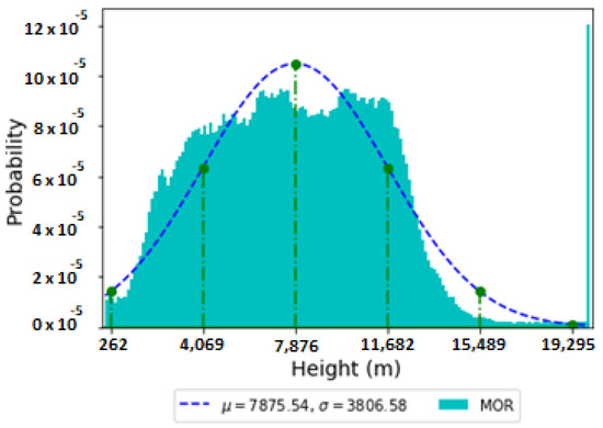
Figure 1.
Histogram on visibility data.
The observation interval of ceilometer backscatter data is irregular at approximately 30 s. The observation interval of AWS data is irregular at 1 h, and the observation interval of visibility sensor data is irregular at 1–3 mins. The intervals of observational data were adjusted to those of the backscatter data.
4.2. Training Data Generation
The training data were generated using denoised backscatter data and weather phenomenon (presence/absence) data. For precipitation, the precipitation sensing value of AWS was used. For fog, AWS and visibility data were used to indicate whether fog occurred. As shown in Table 9, the backscatter coefficients of all heights were used for AWS hourly data.
Table 9.
Field information on train data for weather phenomenon detection.
4.3. Under-Sampling
The number of absent examples was much higher than that of present examples in the training data. Such highly imbalanced data can hinder the training process of machine learning algorithms, making the resulting prediction model rarely predict the present examples. Therefore, we used under-sampling to balance the training data as in [12,31].
The training data comprised data from the first day to the 15th day of each month, and the validation data were composed of data ranging from the 16th to the last day of each month. Random forest was used to find the optimal under-sampling ratio by varying the presence to absence ratio from 1:1 to 1:7. Note that under-sampling is applied only to the training data.
To validate the results, we calculated and compared the accuracy, precision, false alarm rate (FAR), recall (or probability of detection; POD), and F1 score, which are measures that are frequently used in machine learning and meteorology (see Table 10) [32]. Accuracy is the probability that the observed value will coincide with the predicted value among all data ((a + d)/n). In precipitation detection, precision is the probability that the predicted precipitation is correct (a/(a + b)); the FAR is the number of false alarms over the total number of alarms or predicted precipitation samples (b/(a + b)), and recall (or POD) is the fraction of the total amount of precipitation occurrences that were correctly predicted (a/(a + c)). In fog detection, precision is the probability that the predicted fog is correct (a/(a + b)), the FAR is the number of false alarms over the total number of alarms or predicted fog samples (b/(a + b)), and recall (or POD) is the fraction of the total amount of fog occurrences that were correctly predicted (a/(a + c)). F1 score is an index that measures the accuracy of validation, and the harmonic mean of precision and recall (2 × (precision × recall)/(precision + recall)). In imbalanced classification, accuracy can be a misleading metric. Therefore, the F1 score, which considers both precision and recall, is widely used as a major assessment criterion [33,34].
Table 10.
Contingency table for prediction of a binary event. The numbers of occurrences in each category are denoted by a, b, c, and d.
In Table 11 and Table 12, F1 score is the highest when the under-sampling ratio is 1:2. When the under-sampling ratio is 1:7, accuracy is high, but precision is very low. A high precision is good considering the accuracy in the case of precipitation or visibility sensor phenomenon. However, if precision is high, there is a tendency to only overestimate the corresponding phenomenon. Therefore, we selected the case of the highest F1 score whereby precision and recall were balanced. In other words, we under-sampled the precipitation and fog (low visibility) at the under-sampling ratio of 1:2.
Table 11.
Results of precipitation detection according to the under-sampling ratio. The bold number is the best result.
Table 12.
Results of low visibility detection according to the under-sampling ratio. The bold number is the best result.
We also compared our results with two versions of random prediction (see the two bottom rows of Table 11 and Table 12): one method called “Rand” evenly predicts the presence or absence of weather phenomenon at random, and the other method called “W-rand” randomly predicts the presence or absence of weather phenomenon with the weights according to the probability of actual observation of weather phenomenon. We could clearly see that random forest with under-sampling is superior to random prediction with respect to F1 score.
4.4. Feature Selection
A large number of input features significantly increases the computation time of machine learning algorithms and requires an enormous amount of training data to ensure sufficient training. There are 452 input features as shown in Table 9, and these need to be reduced. Figure 2 and Figure 3 show the analyses of denoised backscatter data from 1 January 2015 to 31 May 2016 for precipitation and visibility sensor data, respectively. In Figure 2, ‘True’ indicates the case of precipitation, and ‘False’ indicates the case of non-precipitation. In Figure 3, ‘True’ indicates that the visibility sensor value is equal to or lower than 1000 m, and ‘False’ indicates that the visibility sensor value is higher than 1000 m. The line indicates the backscatter mean value according to height, and the colored part indicates the area of mean ± standard deviation. Above certain heights, it seems difficult to predict the weather phenomena using backscatter data.
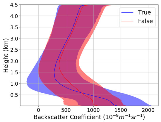
Figure 2.
Backscatter data with precipitation (True) and without precipitation (False).
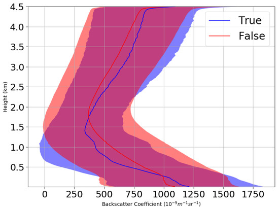
Figure 3.
Backscatter data with low visibility (True) or without low visibility (False).
Therefore, we do not have to use all heights to detect weather phenomena. Random forest was applied after categorizing the total height of 4500 m into 10–300 m, 10–600 m, …, and 10−4500 m while maintaining the under-sampling ratio at 1:2.
Table 13 and Table 14 show that using all the height values ranging from 10 m to 4500 m for precipitation produced satisfactory results. In the case of visibility sensor data, using heights that ranged from 10 m to 3300 m yielded better results than using all the heights that ranged from 10 m to 4500 m. Therefore, the visibility sensor data could yield better results with smaller inputs.
Table 13.
Results of precipitation detection according to feature selection. The bold number is the best result.
Table 14.
Results of low visibility detection according to feature selection. The bold number is the best result.
In the case of precipitation, the number of input features was not reduced by feature selection, and in the case of visibility sensor, the number of input features was reduced to 332, which is not small enough. To train SVM and ANN, we did not use all the heights of the backscatter data. In the case of precipitation, the height intervals of input features were changed from 10 m to 100 m. In other words, we used the backscatter data at 10 m, 110 m, 210 m, …, and 4410 m. For visibility sensor, we used the backscatter data at 10 m, 110 m, …, and 3210 m. Therefore, 47 input features were used to predict precipitation and 35 features to predict fog.
With our final model of random forest preprocessed by under-sampling and feature selection, we provide some observation of representative cases for precipitation and fog in Appendix B.
Table 15 and Table 16 show the results of SVM and ANN. ANN1 is an MLP with one hidden layer whose number of nodes is half of that of the input layer. ANN2 is an MLP with two hidden layers, and the number of nodes at each hidden layer is half that of its input layer. For both precipitation and fog, random forest best classified the weather phenomena, yielding the highest F1 score.
Table 15.
Results of precipitation detection according to other ML techniques.
Table 16.
Results of low visibility detection according to other ML techniques.
5. Concluding Remarks
In this study, we made the first attempt to detect weather phenomena using raw backscatter data obtained from a lidar ceilometer. For weather detection, various machine-learning techniques including under-sampling and feature selection were applied to the backscatter data. The AWS provided observational data for precipitation and the visibility data from PWD20 provided observational data for fog.
Our prediction results were not noticeably good, but if we consider the hardness of weather prediction/detection in the literature (e.g., precision and recall are about 0.5 and 0.3 for heavy rainfall prediction, respectively [13], and they are about 0.2 and 0.5 for lightning forecast, respectively [31]), our prediction results showed potential for precipitation detection (in which precision, recall, and F1 score are about 0.5, 0.2, and 0.3, respectively), but fog detection (in which precision, recall, and F1 score are all about 0.1) was found to be very difficult although it was better than random prediction.
In future work, we expect to improve the accuracy of planetary boundary layer height (PBLH) measurements by classifying backscatter data according to precipitation occurrences.
Author Contributions
Conceptualization, Y.-H.K. and S.-H.M.; methodology, Y.Y. and Y.-H.K.; validation, S.-H.M. and Y.Y.; formal analysis, Y.Y.; investigation, Y.Y. and S.-H.M.; resources, Y.-H.K.; data curation, S.-H.M.; writing—original draft preparation, Y.Y.; writing—review and editing, S.-H.M.; visualization, Y.-H.K.; supervision, Y.-H.K.; project administration, Y.-H.K.; funding acquisition, Y.-H.K. All authors have read and agreed to the published version of the manuscript.
Funding
This work was supported by the Technology Development for Supporting Weather Services, through the National Institute of Meteorological Sciences of Korea, in 2017. This research was also a part of the project titled ‘Marine Oil Spill Risk Assessment and Development of Response Support System through Big Data Analysis’, funded by the Ministry of Oceans and Fisheries, Korea.
Acknowledgments
The authors would like to thank Junghwan Lee and Yong Hee Lee for their valuable helps to greatly improve this paper.
Conflicts of Interest
The authors declare that there is no conflict of interests regarding the publication of this article.
Appendix A. Details of the Used Backscatter Coefficients
In this appendix section, we provide some details of the used backscatter data related to denoising and weather phenomenon, through some representative cases. Figure A1 shows an example of raw backscatter data and their denoised ones which were observed at a moment. We can see that noises are successfully removed. Figure A2 shows an extended time-height plot of raw backscatter data and their denoised ones which had been observed for one day (specifically on 18 March 2015 when daily precipitation was 61 mm). Figure A1 can be understood as a cross section at a point of Figure A2. For Figure A2, we chose a day during which both of precipitation and non-precipitation occurred while clouds are presented in both. In the right side of the figure, a gray box means a period that it rains continuously. We could find clear difference between each box boundary point and its adjacent one, but it does not seem easy to distinguish the two phenomena only by the values themselves.

Figure A1.
Example data of backscatter coefficients at a moment ((left): raw backscatter data and (right): denoised backscatter data).

Figure A2.
Example time-height plotting of backscatter coefficients on 18 March 2015, when both of precipitation and non-precipitation are mixed: a gray box means a precipitation period ((left): raw backscatter data and (right): denoised backscatter data).
Figure A3 shows an example of the denoised backscatter data of CL51 and observation range data of PWD20 which had been observed for one day (specifically on 31 March 2015). For the figure, we chose a day during which both of low visibility and not-low visibility occurred while clouds are presented in both. In the left side of the figure, a gray box means a period that visibility is continuously low (i.e., less than 1000 m). Similar to the precipitation case of Figure A2, it is hard to distinguish the two phenomena only by the values themselves. Moreover, we can see that in the middle period it is not easy even to find some difference between the box boundary point and its adjacent one.

Figure A3.
Example time-height plotting of backscatter coefficients on 31 March 2015, when both of low visibility and not-low visibility are mixed: a gray box means a low visibility period ((left): denoised backscatter data and (right): visibility data).
Appendix B. Case Observation
Figure A4 shows an example of detecting precipitation through backscatter data using random forest. In the case of the left side, the observed weather phenomenon at 15:09:36 (hh:mm:ss) on 21 January 2015 is precipitation and the predicted weather phenomenon is also precipitation. In the case of the right side, the observed weather phenomenon at 23:16:48 on 21 January 2015 is non-precipitation, and the predicted weather phenomenon is precipitation. The blue line indicates the mean value of backscatter data according to the observation value, and the colored part is a section where the standard deviation was added or subtracted from the mean. The distributions of backscatter data are generally similar regardless of precipitation. Since the input of our machine learning model is only backscatter data, it seems natural for the model to output the same prediction result for both cases with similar distribution. Hence, this supports the hardness of predicting precipitation.

Figure A4.
Example of backscatter data predicted as precipitation by machine learning ((left): actual precipitation and (right): actual non-precipitation).
Figure A5 shows an example of detecting non-precipitation from the backscatter data using random forest. In the case of the left side, the observed weather phenomenon at 23:55:12 on is non-precipitation and the predicted weather phenomenon is also non-prediction. In the case of the right side, the observed weather phenomenon at 15:55:48 on 21 January 2015 is precipitation and the predicted weather phenomenon is non-precipitation. Likewise, the distributions of backscatter data are clearly similar regardless of precipitation. As mentioned above, naturally the machine learning model seems to output the same prediction result for both cases. This also supports that it is difficult to predict non-precipitation.

Figure A5.
Example of backscatter data predicted as non-precipitation through machine learning ((left): actual non-precipitation and (right): actual precipitation).
Figure A6 shows an example of detection through the backscatter data using random forest when the visibility sensor value is equal to or less than 1000 m. In the case of the left side, the observed and predicted visibility sensor values at 01:01:46 are both equal to or lower than 1000 m. In the case of the right side, the observed visibility sensor value at 00:46:46 on 22 January 2015 is greater than 1000 m and lower than 20,000 m, and the predicted value is equal to or lower than 1000 m. It is not easy to find clear difference between both cases.

Figure A6.
Example of backscatter data predicted as low visibility by machine learning ((left): actual low visibility and (right): actual not-low visibility).
Figure A7 shows an example of detection from backscatter data using random forest when the visibility sensor value is greater than 1000 m and lower than 20,000 m. In the case of the left side, the observed and predicted visibility sensor values at 00:35:23 on 22 January 2015 are both greater than 1000 m and lower than 20,000 m. In the case of the right side, the observed visibility sensor value at 00:00:00 on 22 January 2015 is 1000 m or lower and the predicted value is greater than 1000 m and lower than 20,000 m. Analogously to the above, we cannot see distinct difference between both cases. It hints that it is very hard to differentiate fog phenomenon by using only backscatter data.

Figure A7.
Example of backscatter data predicted as not-low visibility by machine learning ((left): actual not-low visibility and (right): actual low visibility).
References
- Münkel, C.; Räsänen, J. New optical concept for commercial lidar ceilometers scanning the boundary layer, Remote Sensing. Int. Soc. Opt. Photonics 2004, 5571, 364–374. [Google Scholar]
- Schäfer, K.; Emeis, S.; Rauch, A.; Münkel, C.; Vogt, S. Determination of mixing layer heights from ceilometer data, Remote Sensing. Int. Soc. Opt. Photonics 2004, 5571, 248–259. [Google Scholar]
- Eresmaa, N.; Karppinen, A.; Joffre, S.M.; Räsänen, J.; Talvitie, H. Mixing height determination by ceilometer. Atmos. Chem. Phys. 2006, 6, 1485–1493. [Google Scholar] [CrossRef]
- de Haij, M.; Wauben, W.; Baltink, H.K. Determination of mixing layer height from ceilometer backscatter profiles, Remote Sensing. Int. Soc. Opt. Photonics 2006, 6362, 63620. [Google Scholar]
- Emeis, S.; Schäfer, K. Remote sensing methods to investigate boundary-layer structures relevant to air pollution in cities. Bound. Layer Meteorol. 2006, 121, 377–385. [Google Scholar] [CrossRef]
- Muñoz, R.C.; Undurraga, A.A. Daytime mixed layer over the Santiago basin: Description of two years of observations with a lidar ceilometer. J. Appl. Meteorol. Climatol. 2010, 49, 1728–1741. [Google Scholar] [CrossRef]
- Eresmaa, N.; Härkönen, J.; Joffre, S.M.; Schultz, D.M.; Karppinen, A.; Kukkonen, J. A three-step method for estimating the mixing height using ceilometer data from the Helsinki testbed. J. Appl. Meteorol. Climatol. 2012, 51, 2172–2187. [Google Scholar] [CrossRef]
- Haeffelin, M.; Laffineur, Q.; Bravo-Aranda, J.-A.; Drouin, M.-A.; Casquero-Vera, J.-A.; Dupont, J.-C.; de Backer, H. Radiation fog formation alerts using attenuated backscatter power from automatic lidars and ceilometers. Atmos. Meas. Tech. 2016, 9, 5347–5365. [Google Scholar] [CrossRef]
- Cazorla, A.; Casquero-Vera, J.A.; Román, R.; Guerrero-Rascado, J.L.; Toledano, C.; Cachorro, V.E.; Orza, J.A.G.; Cancillo, M.L.; Serrano, A.; Titos, G.; et al. Near-real-time processing of a ceilometer network assisted with sun-photometer data: Monitoring a dust outbreak over the Iberian Peninsula. Atmos. Chem. Phys. 2017, 17, 11861–11876. [Google Scholar] [CrossRef]
- Chan, K.L.; Wiegner, M.; Flentje, H.; Mattis, I.; Wagner, F.; Gasteiger, J.; Geiß, A. Evaluation of ECMWF-IFS (version 41R1) operational model forecasts of aerosol transport by using ceilometer network measurements. Geosci. Model Dev. 2018, 11, 3807–3831. [Google Scholar] [CrossRef]
- Lee, S.; Hwang, S.-O.; Kim, J.; Ahn, M.-H. Characteristics of cloud occurrence using ceilometer measurements and its relationship to precipitation over Seoul. Atmos. Res. 2018, 201, 46–57. [Google Scholar] [CrossRef]
- Seo, J.-H.; Lee, Y.H.; Kim, Y.-H. Feature selection for very short-term heavy rainfall prediction using evolutionary computation. Adv. Meteorol. 2014, 2014, 203545. [Google Scholar] [CrossRef]
- Moon, S.-H.; Kim, Y.-H.; Lee, Y.H.; Moon, B.-R. Application of machine learning to an early warning system for very short-term heavy rainfall. J. Hydrol. 2019, 568, 1042–1054. [Google Scholar] [CrossRef]
- Lee, M.-K.; Moon, S.-H.; Yoon, Y.; Kim, Y.-H.; Moon, B.-R. Detecting anomalies in meteorological data using support vector regression. Adv. Meteorol. 2018, 2018, 5439256. [Google Scholar] [CrossRef]
- Kim, H.-J.; Park, S.M.; Choi, B.J.; Moon, S.-H.; Kim, Y.-H. Spatiotemporal approaches for quality control and error correction of atmospheric data through machine learning. Comput. Intell. Neurosci. 2020, 2020, 7980434. [Google Scholar] [CrossRef] [PubMed]
- Lee, M.-K.; Moon, S.-H.; Kim, Y.-H.; Moon, B.-R. Correcting abnormalities in meteorological data by machine learning. In Proceeding of the IEEE International Conference on Systems, Man, and Cybernetics, San Diego, CA, USA, 5–8 October 2014; pp. 902–907. [Google Scholar]
- Kim, Y.-H.; Ha, J.-H.; Yoon, Y.; Kim, N.-Y.; Im, H.-H.; Sim, S.; Choi, R.K.Y. Improved correction of atmospheric pressure data obtained by smartphones through machine learning. Comput. Intell. Neurosci. 2016, 2016, 9467878. [Google Scholar] [CrossRef]
- Ha, J.-H.; Kim, Y.-H.; Im, H.-H.; Kim, N.-Y.; Sim, S.; Yoon, Y. Error correction of meteorological data obtained with Mini-AWSs based on machine learning. Adv. Meteorol. 2018, 2018, 7210137. [Google Scholar] [CrossRef]
- Moon, S.-H.; Kim, Y.-H. An improved forecast of precipitation type using correlation-based feature selection and multinomial logistic regression. Atmos. Res. 2020, 240, 104928. [Google Scholar] [CrossRef]
- Breiman, L. Random forests. Mach. Learn. 2001, 45, 5–32. [Google Scholar] [CrossRef]
- Cortes, C.; Vapnik, V. Support-vector networks. Mach. Learn. 1995, 20, 273–297. [Google Scholar] [CrossRef]
- Jain, A.K.; Mao, J.; Mohiuddin, K.M. Artificial neural networks: A tutorial. IEEE Comput. 1996, 29, 31–44. [Google Scholar]
- Gardner, M.W.; Dorling, S.R. Artificial neural networks (the multilayer perceptron)—A review of applications in the atmospheric sciences. Atmos. Environ. 1998, 32, 2627–2636. [Google Scholar]
- Korea Meteorological Administration. Available online: http://www.kma.go.kr (accessed on 10 July 2020).
- Vaisala, CL51. Available online: https://www.vaisala.com/en/products/instruments-sensors-and-other-measurement-devices/weather-stations-and-sensors/cl51 (accessed on 10 July 2020).
- Münkel, C.; Roininen, R. Investigation of boundary layer structures with ceilometer using a novel robust algorithm. In Proceedings of the 15th Symposium on Meteorological Observation and Instrumentation, Atlanta, GA, USA, 16–21 January 2010. [Google Scholar]
- Ha, J.-H.; Kim, Y.-H.; Lee, Y.H. Applying artificial neural networks for estimation of planetary boundary layer height. J. Korean Inst. Intell. Syst. 2017, 27, 302–309. (In Korean) [Google Scholar] [CrossRef]
- Vincent, P.; Larochelle, H.; Lajoie, I.; Bengio, Y. Stacked denoising Autoencoders: Learning Useful Representations in a Deep Network with a Local denOising Criterion. J. Mach. Learn. Res. 2010, 11, 3371–3408. [Google Scholar]
- Vaisala PWD20. Available online: https://www.vaisala.com/en/products/instruments-sensors-and-other-measurement-devices/weather-stations-and-sensors/pwd10-20w (accessed on 10 July 2020).
- American Meteorological Society, Fog, Glossary of Meteorology. Available online: http://glossary.ametsoc.org/wiki/fog (accessed on 10 July 2020).
- Moon, S.-H.; Kim, Y.-H. Forecasting lightning around the Korean Peninsula by postprocessing ECMWF data using SVMs and undersampling. Atmos. Res. 2020, 243, 105026. [Google Scholar] [CrossRef]
- Goutte, C.; Gaussier, E. A probabilistic interpretation of precision, recall and F-score, with implication for evaluation. Lect. Notes Comput. Sci. 2005, 3408, 345–359. [Google Scholar]
- Sun, Y.; Kamel, M.S.; Wong, A.K.; Wang, Y. Cost-sensitive boosting for classification of imbalanced data. Pattern Recognit. 2007, 40, 3358–3378. [Google Scholar]
- Liu, X.-Y.; Wu, J.; Zhou, Z.-H. Exploratory undersampling for class-imbalance learning. IEEE Trans. Syst. Man Cybern. Part B Cybern. 2009, 39, 539–550. [Google Scholar]
© 2020 by the authors. Licensee MDPI, Basel, Switzerland. This article is an open access article distributed under the terms and conditions of the Creative Commons Attribution (CC BY) license (http://creativecommons.org/licenses/by/4.0/).