Long Wave Run-Up Resonance in a Multi-Reflection System

Abstract

Wave reflection and wave trapping can lead to long wave run-up resonance. After reviewing the theory of run-up resonance in the framework of the linear shallow water equations, we perform numerical simulations of periodic waves incident on a linearly sloping beach in the framework of the nonlinear shallow water equations. Three different types of boundary conditions are tested: fully reflective boundary, relaxation zone, and influx transparent boundary. The effect of the boundary condition on wave run-up is investigated. For the fully reflective boundary condition, it is found that resonant regimes do exist for certain values of the frequency of the incoming wave, which is consistent with theoretical results. The influx transparent boundary condition does not lead to run-up resonance. Finally, by decomposing the left- and right-going waves into a multi-reflection system, we find that the relaxation zone can lead to run-up resonance depending on the length of the relaxation zone.

1. Introduction

Long wave run-up is difficult to observe in nature in real-time due to the catastrophic consequences it usually leads to. An illustration of a long wave is a tsunami, which has a wavelength far greater than the water depth and a small amplitude in the open ocean. When a tsunami reaches the nearshore region, its amplitude increases significantly, while its propagation speeds decreases. A large part of the theoretical results for run-up are based on shallow water theory. Analytical linear solutions for periodic long waves on a slope can be found, for example, in Green and Ferrers [1], Lamb [2], and Keller and Keller [3].

Tsunamis are known for their dramatic run-up height. From the data collection of post-tsunami surveys, extreme run-up values have been observed that exceed 20m and the most severe damages were not always caused by the first wave [4,5,6]. Extreme run-up values cannot be explained by classical analytical solutions. A possible explanation for these extreme run-ups is resonance. Miles [7] and Wilson [8] discussed the conditions for resonance in closed and open basins. The Helmholtz mode was also studied, which is the most important mode in natural basins and is normally observed in bays, inlets, and harbors with narrow entrance. Kajiura [9] described the possibility of resonances in bays. Rabinovich and Leviant [10] introduced the concept of shelf resonance, which is also called quarter-wavelength resonance. Neetu et al. [11] found that reflection and refraction from the nearshore topographic features can lead to the amplification of run-up values of non-leading tsunami waves. Resonance effects in the process of run-up have been studied numerically by Stefanakis et al. [12,13] and experimentally by Abcha et al. [14,15].

Obviously boundary conditions play an important role in numerical simulations: they can easily make the difference between successful and unsuccessful computations, or between fast and slow ones. There is still no clear understanding of how to impose both incoming and outgoing waves at a boundary. One generally uses an open boundary condition seaward, which is a numerical artifact that lies in a limited computational domain to solve a mathematical problem that has no boundary at all. Such open boundary conditions are usually called “radiation”, “absorbing”, “non-reflecting”, or “far-field” boundary conditions. They all allow waves to leave the truncated domain, thus avoiding spurious reflections that may pollute the solution in the interior of the computational domain of interest. They can be classified into two groups: non-reflecting boundary conditions and non-reflecting boundary layers. Non-reflecting boundary conditions absorb impinging waves on the artificial boundary. A classical example is the Sommerfeld boundary condition [16,17]. On the other hand, non-reflecting boundary layers have the property of absorbing waves that are traveling inside the layer. Open boundaries are considered in a widespread literature. Examples are Jensen [18], Carter and Merrifield [19], Ma and Madsen [20].

However, in a laboratory wave flume, not all reflections caused by a wave paddle can be eliminated. The resulting wave system is a multi-reflection system. In the framework of wave energy converters, Wei et al. [21] discussed the re-reflection effects on the wave field. In nature, waves on some topographies are easily trapped, such as in narrow bays. When the water depth changes abruptly in shelves with piece-wise geometry, a multi-reflection system can also occur. Such reflective boundary conditions are seldom discussed.

Run-up on a sloping beach with the use of an open boundary condition at the seaward boundary matches the linear analytical solution that shows no resonance at all. However, no matter if it is theory or experiment, there exist some resonant frequencies [2,13,22]. Wave trapping is one of the phenomena that lead to resonance [23,24]. Using reflective boundary conditions leads to the reflection of outgoing waves and leaves them in the computational domain, thus constructing a multi-reflection system. We discuss run-up in such a system.

In this paper, we provide the analytical solution of run-up on a bounded domain that consists of a sloping beach connected to a flat bottom (linear shallow water equations). Conditions for run-up resonance are given. Then, we investigate numerically the same problem (nonlinear shallow water equations) using three different boundary conditions: influx transparent boundary conditions, reflective boundary conditions, and relaxation zones. The outcome of the numerical simulations is shown. For the fully reflective boundary condition, it is found that resonant regimes do exist for certain values of the frequency of the incoming wave, which is consistent with theoretical results. The influx transparent boundary condition does not lead to run-up resonance. By decomposing the left- and right-going waves into a multi-reflection system, we find that the relaxation zone can lead to run-up resonance depending on the length of the relaxation zone. Finally, the applicability of the results to tsunami science is briefly discussed.

2. Materials and Methods

We consider periodic waves of angular frequency $\omega$ incident on a linearly sloping beach with angle $\alpha$ (see Figure 1). The sloping beach starts at a distance L from the shore.

The one-dimensional (1D) nonlinear shallow water equations (NSWE) read

$$\frac{\partial \eta }{\partial t}+\frac{\partial }{\partial x}(hu)=0,$$

(1)

$$\frac{\partial u}{\partial t}+u\frac{\partial u}{\partial x}+g\frac{\partial \eta }{\partial x}=0,$$

(2)

where x is the horizontal coordinate, t is time, $\eta (x,t)$ is the free-surface elevation, $h(x,t)=h_0(x)+\eta (x,t)$ is the water depth with $h_0(x)$ the still water depth, $u(x,t)$ is the depth-averaged horizontal velocity, and g is the acceleration due to gravity. The origin of the coordinate system is at the shoreline. The still water depth $h_0(x)$ is equal to $Ltan\alpha$ for $-L_t\le x\le -L$ and $-xtan\alpha$ for $-L\le x\le 0$.

2.1. Theoretical Model for Run-Up Resonance Based on the Linear Shallow Water Equations

Resonance phenomena play an important role in run-up amplification. They can explain extreme run-up heights and later arrival of waves with larger amplitude. For the geometry of Figure 1, Billingham and King [25] used linear shallow water theory to show that a resonance occurs when $2\omega \sqrt{L/(gtan\alpha )}$ is a zero of the Bessel function $J_0$. This resonance can also be found both in the numerical results of Stefanakis et al. [13] and in the experimental results of Ezersky et al. [22], because of the presence of a reflective boundary condition seaward.

Even though the numerical simulations shown in the next section are based on the 1D NSWE (1) and (2), we use the 1D linear shallow water equations (LSWE) to explain the resonance phenomenon analytically. The 1D LSWE read

$$\frac{\partial \eta }{\partial t}+\frac{\partial }{\partial x}(h_{0}u)=0,$$

(3)

$$\frac{\partial u}{\partial t}+g\frac{\partial \eta }{\partial x}=0.$$

(4)

The phase velocity of the wave is denoted by $c(x)=\omega /k(x)=\sqrt{g{h}_0(x)}$.

Equations (3) and (4) can be combined into a single equation:

$$\frac{{\partial }^2\eta }{\partial t^2}-g\frac{\partial }{\partial x}\left(h_0\frac{\partial \eta }{\partial x}\right)=0.$$

(5)

For a beach with a constant slope, we look for a harmonic solution of the form [26]

$$\eta (x,t)=\mathcal{A}(x)e^{-i\omega t}.$$

(6)

Inserting Equation (6) into Equation (5) leads to

$$\frac{d^2\mathcal{A}}{d{\sigma }^2}+\frac{1}{\sigma }\frac{d\mathcal{A}}{d\sigma }+\mathcal{A}=0,$$

(7)

where $\sigma ={\int }_0^{x}k(x)dx$ with $k(x)$ the wave number. Equation (7) is the Bessel equation of the first kind, whose solution can be represented by

$$\mathcal{A}=A_1{J}_0(\sigma )+A_2{Y}_0(\sigma ),$$

(8)

where $A_1$ and $A_2$ are linear coefficients, and $J_0$, resp. $Y_0$, are the Bessel functions of the first and second kind. As $Y_0$ tends to infinity at the shore, the coefficient of $Y_0$ must be zero in the nearshore region if we assume that the amplitude of the free-surface elevation is finite. Therefore, $\mathcal{A}$ is expressed only in terms of the Bessel function of the first kind:

$$\mathcal{A}=R_{max}{J}_0(\sigma ),$$

(9)

where $R_{max}$ denotes the run-up. Billingham and King [25] found the resonance mentioned above by imposing a fixed amplitude at $x=L$. Indeed, $\sigma (x=L)=2\omega \sqrt{L/(gtan\alpha )}$.

For a constant-depth region, the wave field can be described as a sum of incident and reflected waves:

$$\eta (x,t)=(A_i{e}^{-ikx}+A_r{e}^{ikx})e^{-i\omega t},$$

(10)

where $A_i$ and $A_r$ are the amplitudes of the incident and reflected waves, respectively.

Next, we discuss run-up due to the more realistic bathymetry profile that consists of a constant depth region connected to a sloping beach. Hereafter, it will be referred to as the canonical case (see Figure 1). Following Kanoğlu and Synolakis [27] and Stefanakis et al. [13], we use the continuity of the free-surface elevation and of the horizontal fluxes to match surface elevations (Equation (11)) and particle velocities (according to Equation (4), it is equivalent to Equation (12)) at the toe of the sloping beach from two adjacent segments, and match the surface elevations at the left boundary Equation (13), respectively. We obtain

$$\begin{array}{ccc}\hfill J_0({\sigma }_1)R_{max}-J_0({\sigma }_2)A_1-Y_0({\sigma }_2)A_2& =& 0,\hfill \end{array}$$

(11)

$$\begin{array}{ccc}\hfill J_1({\sigma }_1)R_{max}-J_1({\sigma }_2)A_1-Y_1({\sigma }_2)A_2& =& 0,\hfill \end{array}$$

(12)

$$\begin{array}{cccc}\hspace{1em}\hspace{1em}\hspace{1em}\hspace{1em}\hspace{1em}\hspace{1em}\hspace{1em}\hspace{1em}\hspace{1em}\hspace{1em} & \hfill J_0({\sigma }_3)A_1+Y_0({\sigma }_3)A_2& =& \hfill A_i{e}^{-ikx}+A_r{e}^{ikx},\end{array}$$

(13)

where

$$\begin{array}{ccc}\hfill {\sigma }_1& =& 2\omega \sqrt{\frac{L}{gtan\alpha }},\hfill \end{array}$$

(14)

$$\begin{array}{ccc}\hfill {\sigma }_2& =& \frac{\omega L}{\sqrt{gLtan\alpha }},\hfill \end{array}$$

(15)

$$\begin{array}{ccc}\hfill {\sigma }_3& =& \frac{\omega L_t}{\sqrt{gLtan\alpha }}.\hfill \end{array}$$

(16)

The determinant of the system (11)–(13) is given by

$$det(\mathrm{system})=\left|\begin{array}{ccc}{J}_0({\sigma }_1)& -J_0({\sigma }_2)& -Y_0({\sigma }_2)\\ J_1({\sigma }_1)& -J_1({\sigma }_2)& -Y_1({\sigma }_2)\\ 0& J_0({\sigma }_3)& Y_0({\sigma }_3)\end{array}\right|·$$

(17)

When the determinant vanishes, run-up becomes resonant. Therefore, the resonance condition reads $det(\mathrm{system})=0$. Clearly, the distance $L_t$ from the shore to the seaward boundary that appears in ${\sigma }_3$ plays a crucial role in the resonance condition.

2.2. Numerical Integration of the Nonlinear Shallow Water Equations—The Boundary Conditions

We integrate the 1D NSWE (1) and (2) with a finite volume solver based on the Characteristic Flux scheme with UNO2 reconstruction for higher order terms. A third-order Runge–Kutta scheme is used for time discretization. The numerical model is described and validated in Dutykh et al. [28]. What is new here is the fact that we test three types of boundary conditions described below.

2.2.1. Influx Transparent Boundary Conditions

Appropriate boundary conditions are needed to let the wave travel in and out of the domain in an undisturbed way. Influx transparent boundary conditions are boundary conditions that make waves on boundaries propagate into the computational domain and are transparent for wave propagation out of the computational domain. In the region of constant depth, the LSWE reduce to two wave Equations [2]:

$${\eta }_{tt}-c^2{\eta }_{xx}=0,$$

(18)

and

$${\mathsf{\Phi }}_{tt}-c^2{\mathsf{\Phi }}_{xx}=0,$$

(19)

where $\mathsf{\Phi }$ is the time-integral of the displacement past the plane x, up to the time t: $\mathsf{\Phi }(x,t)={\int }^{t}udt$.

Equations (18) and (19) have the general solutions

$$\begin{array}{ccc}\hfill \eta (x,t)& =& {\eta }_{rg}(\frac{x}{c}-t)+{\eta }_{lg}(\frac{x}{c}+t),\hfill \end{array}$$

(20)

$$\begin{array}{ccc}\hfill \mathsf{\Phi }(x,t)& =& {\mathsf{\Phi }}_{rg}(\frac{x}{c}-t)+{\mathsf{\Phi }}_{lg}(\frac{x}{c}+t),\hfill \end{array}$$

(21)

where the subscripts $lg$ and $rg$ denote the waves traveling to the left and to the right directions, respectively.

Differentiating Equation (21) with respect to x and t yields

$$\begin{array}{ccc}\hfill {\mathsf{\Phi }}_x& =& \frac{1}{c}{\mathsf{\Phi }}_{rg}^{\prime }+\frac{1}{c}{\mathsf{\Phi }}_{lg}^{\prime },\hfill \end{array}$$

(22)

$$\begin{array}{ccc}\hfill {\mathsf{\Phi }}_t& =& -{\mathsf{\Phi }}_{rg}^{\prime }+{\mathsf{\Phi }}_{lg}^{\prime }.\hfill \end{array}$$

(23)

To build a left boundary at $x=x_l$ that is transparent for waves propagating to the left but allows waves to propagate to the right, we eliminate ${\mathsf{\Phi }}_{lg}^{\prime }$:

$${\mathsf{\Phi }}_t-c{\mathsf{\Phi }}_x{\mid }_{x=x_l}=-2{\mathsf{\Phi }}_{rg}^{\prime }{\mid }_{x=x_l}.$$

(24)

This is called the left Influx Transparent Boundary Condition (ITBC).

As ${\mathsf{\Phi }}_t=u$,

$$\begin{array}{c}\hfill u(x_l,t)=c{\mathsf{\Phi }}_x{\mid }_{x=x_l}-2{\mathsf{\Phi }}_{rg}^{\prime }{\mid }_{x=x_l}.\end{array}$$

(25)

Moreover, from (3),

$$\begin{array}{c}\hfill {\mathsf{\Phi }}_x={\int }^t{u}_{x}dt=-\frac{1}{h_0}\eta =-\frac{g}{c^2}\eta .\end{array}$$

(26)

Therefore, the velocity at the left boundary can be written as

$$u(x_l,t)=-\frac{g\eta (x_l,t)}{c(x_l)}+\frac{2g{\eta }_{rg}(x_l,t)}{c(x_l)}.$$

(27)

Similarly, the right ITBC $(x=x_r)$ that is transparent for waves propagating to the right but makes waves propagate to the left can be written as

$${\mathsf{\Phi }}_t+c{\mathsf{\Phi }}_x{\mid }_{x=x_r}=2{\mathsf{\Phi }}_{lg}^{\prime }{\mid }_{x=x_r}.$$

(28)

Therefore, the velocity at the right boundary is

$$u(x_r,t)=\frac{g\eta (x_r,t)}{c(x_r)}-\frac{2g{\eta }_{lg}(x_r,t)}{c(x_r)}.$$

(29)

The head-on collision of two single waves on a flat bottom with the use of the left and right influx transparent boundary conditions is shown in Figure 2. Waves of the form ${\eta }_0(t)=0.1$ sech ${}^2(0.17t-2)$ are generated at the boundaries. As the boundaries are transparent to the outgoing waves, no reflection occurs at the boundaries.

2.2.2. The Reflective Boundary Conditions

The reflective boundary conditions are boundary conditions that are prescribed on a bounded interval $[x_l,x_r]$ and read

$$\begin{array}{c}\hfill {\eta }_x(x_l,t)={\eta }_x(x_r,t)=0,\end{array}$$

(30)

$$\begin{array}{c}\hfill u(x_l,t)=u(x_r,t)=0.\end{array}$$

(31)

For the classical NSWE system, we only need to impose the boundary conditions in one of the two dependent variables [29]. Therefore, it is sufficient to take $u(x_l,t)=u(x_r,t)=0$ as reflective boundary condition.

In this paper, analogous reflective boundary conditions are considered. The incident wave $\eta (x_l,t)$ is coming from the left boundary, where the velocity can be expressed by

$$u(x_l,t)=c(x_l,t)+\left(1-\frac{h(x_l,t)}{H(x_l,t)}\right)c(x_l,t),$$

(32)

where $h(x,t)$ is the total depth of water and $H(x_l,t)=h_0+{\eta }_i(t)$ with ${\eta }_i(t)$ the free-surface elevation of the incident wave at the left boundary. This boundary condition was used by Stefanakis et al. [12]. A vertical wall is used at the right boundary, which means $u(x_r,t)=0$. Figure 3 shows an incident single wave generated at the left boundary that propagates to the right and meets a vertical wall at the right boundary, where it is reflected. When the reflected wave propagates back towards the left boundary, it reflects again and the wave polarity is reversed. It makes a multi-reflection system.

2.2.3. The Relaxation Zone

The relaxation zone is a kind of non-reflecting boundary layer. It absorbs all the reflected waves in a region that lies at the inlet boundary. It is usually one wavelength long [26,30]. In practice, it can modify an incident wave field to any desired target function. This also extends the applicability of the sponge layer to inlet boundaries, as the target function could be that of the generated wave train. The relaxation zone works as a blend between a target solution and the computed solution. The modified velocity can be described by

$$u=c_{relax}{u}_{target}+(1-c_{relax})u_{model},$$

(33)

where $u_{target}$ is a target velocity, $u_{model}$ is the unaltered computed velocity, and $c_{relax}$ is the relaxation coefficient. This technique has been discussed in many papers, such as Mayer et al. [31,32,33,34,35]. As the relaxation is applied explicitly as a postprocessing step, it is possible to apply it at the inlet. If there is no proper relaxation, the waves may propagate upstream toward the inlet boundary, be reflected back into the computational domain and pollute the flow field.

To obtain a smoothly modified internal flow field, it is required that “$c_{relax}$” and its spatial derivatives are equal to zero along the interface connecting the relaxation zone and the internal field of the computational domain. There are many options to build a proper function of the relaxation coefficient. In this paper, we use the form

$$c_{relax}(\beta )=b{\beta }^3+(1-b){\beta }^6,$$

(34)

where $b\in [0,2]$ is a free parameter, and $\beta =1-(x-x_{start})/(x_{end}-x_{start})$ ($x_{start}$ and $x_{end}$ are coordinates of the relaxation zone boundaries) is the nondimensional distance function.

The choice of the relaxation coefficient $c_{relax}$ depends strongly on the problem and the length of the relaxation zone. What is important is that the choice is not unique for a given problem.

In numerical simulations, reflected waves from the beach will interact with the wave generation boundary, which will pollute the final results, especially for breaking waves. Therefore, we can test the applicability of the relaxation zone through the modeling of standing waves. If it can absorb reflected waves in front of the inlet, the incident wave profile is kept in the relaxation zone and the standing wave pattern is simulated in the non-relaxed part of the computational zone.

The standing wave is modeled as sketched in Figure 4. The relaxation zone at the left boundary is one wavelength long. The total horizontal length of the domain is three wavelengths. The incident wave amplitude is ${\eta }_0=1$ m, the wave period is $T=40$ s, and the water depth is $h_0=20$ m. One can see that the relaxation zone can simulate a standing wave pattern well in the non-relaxed part of the computational domain.

The relaxation zone makes the boundary as “open”. Compared with the ITBC, which can only be applied to regular waves, it can be wildly used for any type of wave, regular or irregular, long or short.

3. Results for Waves Incident on a Linearly Sloping Beach

Having described the three types of boundary conditions, we now present their effect on the numerical simulations of waves incident on a linearly sloping beach. Periodic monochromatic incident waves $\eta (x_l,t)={\eta }_{0}sin(\omega t)$ propagate towards a sloping beach, with sloping angle $tan\alpha =0.02$ (unless otherwise specified) and horizontal length $L=5000$ m (unless otherwise specified). The value $tan\alpha =0.02$ is typical of nearshore conditions as seen in [36].

3.1. Results with the Influx Transparent Boundary Conditions

The left ITBC is used on the left boundary. Non-dimensional run-up with respect to nondimensional wavelength is shown in Figure 5. One can see that the numerical nondimensional run-up matches the results given by the analytical linear solution before wave breaking. The ITBC is only approximate when the wavelength is too large as can be seen in Figure 5 for ${\lambda }_0/L>3$ [23,37,38]. The left boundary is not entirely transparent to outgoing waves when the wavelength is large. The outgoing waves are partially reflected and trapped in the computational domain. However, the effect on run-up is slight.

3.2. Results with the Reflective Boundary Conditions

We construct a multi-reflection system for the canonical case of Figure 1, where the reflective boundary conditions are used. Waves generated at the left seaward boundary propagate forward and are reflected at the right boundary. The reflected waves propagate back to the left boundary and are re-reflected, then the re-reflected waves propagate forward again and the process is repeated. A reflection cycle is defined as a cycle during which the wave travels the total domain back and forth. The time it takes is called the reflection period $T_{reflect}$. For the canonical case of Figure 1, it can be expressed by

$$T_{reflect}=2\left(\frac{L_t-L}{\sqrt{g{h}_0}}+\frac{2L}{\sqrt{g{h}_0}}\right).$$

(35)

In the simulations below, the total simulation time is always four reflection cycles, and the incident periodic wave at $x=-L_t$ is expressed by

$${\eta }_i(t)={\eta }_{0}sin\left(\frac{2\pi t}{T}\right),$$

(36)

where T is the wave period and ${\eta }_0=0.1$ m.

First, we considered three combinations of $\alpha$, L, and $L_t$, thus fixing $T_{reflect}$ for each combination. We tested the maximum run-up in a multi-reflection system for three cases by varying the nondimensional wave period within the range $0.25<T/T_{reflect}<0.65$ (see Figure 6). Resonance effects are clearly visible. The maximum nondimensional run-ups are sharply amplified for certain wave periods, which lead to three peaks in Figure 6a, i.e., the maximum nondimensional run-up is up to 27 when $tan\alpha$ = 0.02, $L_t$ = 8000 m, L = 5000 m, and T = 220.8 s $(T/T_{reflect}$ = 0.2658). Second, we fixed $\alpha$, L, and T instead of $L_t$, the horizontal distance from the left boundary to the undisturbed shoreline. This time, we tested the maximum run-up as a function of $L_t$, which in turn made $T_{reflect}$ and $T/T_{reflect}$ vary through Equation (35). The results are shown in Figure 7. Waves with the same period propagating on the same bathymetry ($tan\alpha$ = 0.02, L = 2000 m) lead to different maximum run-ups with respect to various flat bottom lengths, which indicates that the wave behavior is affected by the location of the left boundary. This is different from the open boundary. However, resonance occurs when $T/T_{reflect}=0.2658,0.3595$ in the range of $0.25<T/T_{reflect}<0.4$. From these two figures, monochromatic forcing is found to lead to resonant run-up by non-leading waves when the nondimensional wave periods $T/T_{reflect}$ are the roots of the determinant of system (17), which coincides with the resonance condition we gave above.

3.3. Results with the Relaxation Zone

Next, we investigate the wave behavior in the presence of a relaxation zone. Its coefficients are given in the equation for $c_{relax}$ (34). However, we use the parameters $b=2$ and $\beta =(x_{end}-x)/{\lambda }_0$, where ${\lambda }_0$ is the wavelength of the incoming wave. When the full relaxation zone is applied, the value of “$c_{relax}$” decreases from 1 to 0 along the relaxation zone. When the relaxation zone is only partial, the value of “$c_{relax}$” decreases from a value that depends on the length of the zone (value less than 1) to 0.

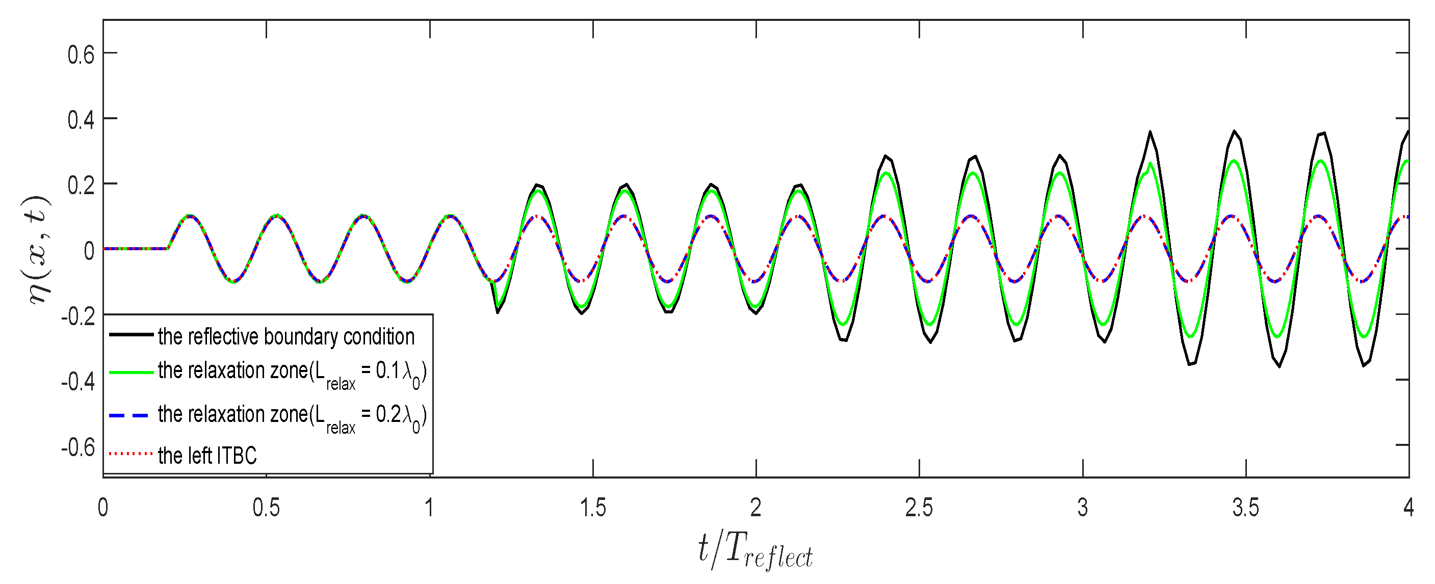
Results are shown in Figure 8. Two different relaxation zones are considered. To emphasize the effect of the relaxation zone, we also show the free-surface elevation time series with the use of the other boundary conditions described above (reflective and left ITBC). One can observe that the partial relaxation zone only alters the wave amplitude, but maintains the other wave characteristics. In other words, it can be considered as a partially reflective boundary condition. When the length of the relaxation zone is one fifth of the incident wavelength, the results coincide with those of obtained with the left ITBC, which means that there is no reflection caused at the left boundary.

4. Conditions for Run-Up Resonance in a Multi-Reflection System

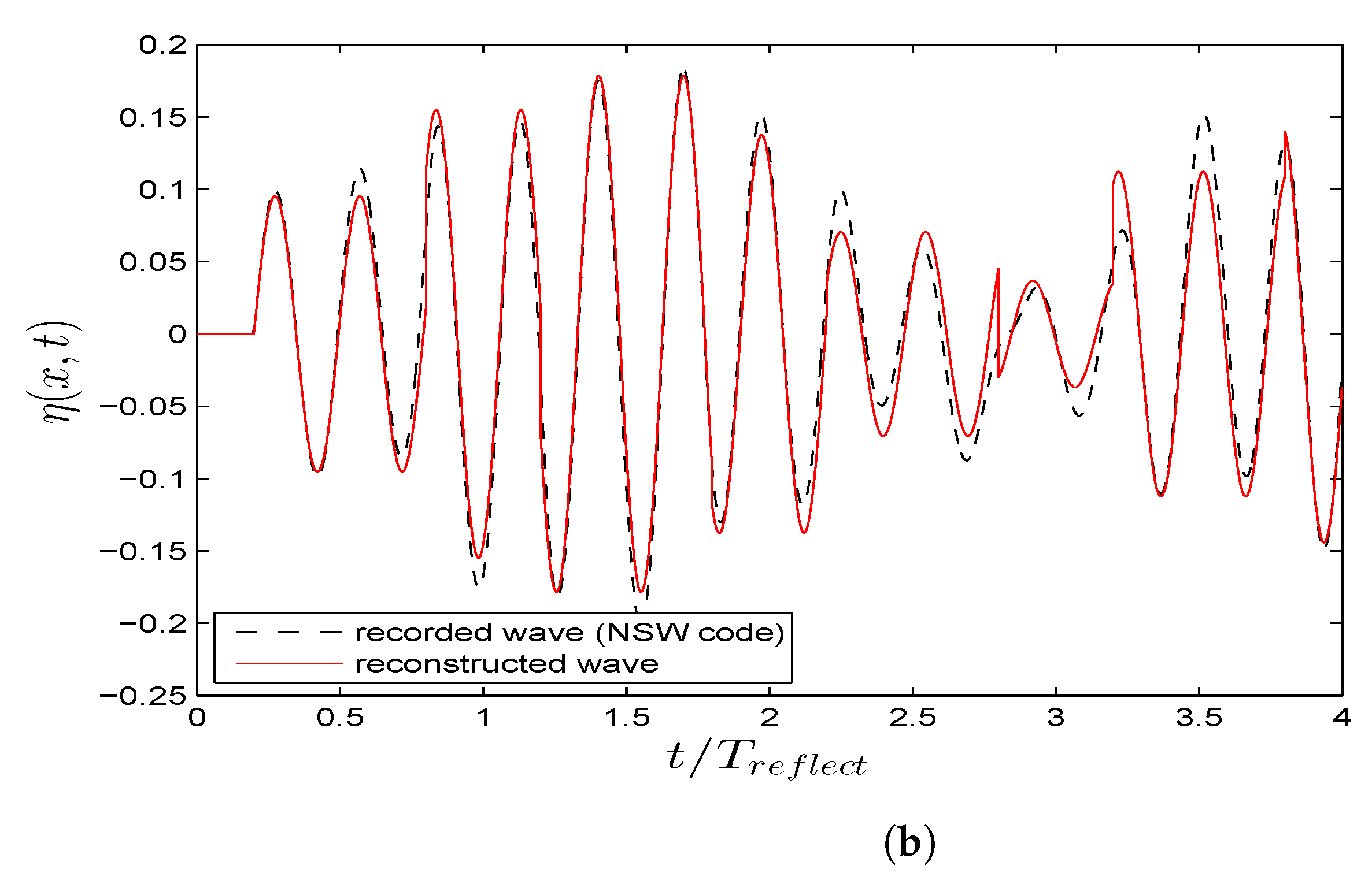
To investigate the influence of the boundary conditions on the resonance mechanism, we first consider the reflective boundary conditions. In Appendix A, we describe a technique to decompose a wave into left- and right-going waves in a multi-reflection system. Using that technique, we separated the recorded waves at a point x located 2000 m to the right of the left boundary, into left- and right-going waves with $L_t=7000,8000,9000$ m. The other parameters were fixed at $L=2000$ m, $tan\alpha =0.02$, $T=268.5$ s, and ${\eta }_0=0.1$ m (see Figure 9). The amplitudes of left- and right-going waves are constant in each reflection cycle. When $L_t=8000$ m, the amplitude of right-going waves is the sum of amplitudes of the initial incident wave and of the left-going wave in the preceding reflection cycle, which are not observed in the other two cases (see Figure 9).

The wave motion could develop as a standing wave pattern with the use of open boundary condition [26]. For a multi-reflection system, it can be considered as a superposition of a standing wave and traveling waves. When the phase difference between the right-going and left-going waves is $\pi$, resonance can occur. When $L_t$ = 8000 m, one can observe that the phase difference between the right-going and left-going waves is close to $\pi$ (see Figure 9b,c), which leads to resonance and amplifies the free surface elevation significantly (see Figure 9a). The period T = 268.5 s ($T/T_{reflect}=0.2658$) used in Figure 9 is the resonant frequency that leads to the first peak in Figure 6a. Therefore, det(system) = 0 gives an analytical resonance condition, and Figure 9 reveals a wave motion resonance condition. We can conclude that the phase difference between the right-going and left-going waves must be $\pi$ for the waves of the periods at the run-up peaks and det(system) = 0 in Figure 7.

Due to the new incident component coming from the reflected component in the previous reflection cycle, the reflection coefficient $r_l^{(m)}$ in the mth reflection cycle at the left boundary can be defined by

$$r_l^{(m)}=\frac{A_I^{(1,m)}}{A_R^{(1,m-1)}},$$

(37)

where $m>1$. The average value is considered as the reflection coefficient of the left boundary.

Table 1. Reflection coefficients at the left boundary with four boundary conditions for the canonical case, when $L_t=8000$ m, $L=2000$ m, $tan\alpha =0.02$, and $T=268.5$ s ($T/T_{reflect}=0.2658$).

	Reflective Boundary Condition	Partial Relaxation Zone (${\mathit{L}}_{\mathit{relax}}=\mathbf{0.1}{\mathit{\lambda }}_{\mathbf{0}}$)	Partial Relaxation Zone (${\mathit{L}}_{\mathit{relax}}=\mathbf{0.2}{\mathit{\lambda }}_{\mathbf{0}}$)	Left ITBC
$m=1$	—	—	—	—
$m=2$	0.9718	0.7419	—	—
$m=3$	0.9725	0.7380	—	—
$m=4$	0.9500	0.7219	—	—
reflection coefficients	0.9648	0.7339	no reflection	no reflection

and

Table 2. Reflection coefficients at the left boundary with four boundary conditions for the canonical case, when $L_t=7000$ m, $L=200$0 m, $tan\alpha =0.02$, and $T=268.5$ s ($T/T_{reflect}=0.2953$).

	Reflective Boundary Condition	Partial Relaxation Zone (${\mathit{L}}_{\mathit{relax}}=\mathbf{0.1}{\mathit{\lambda }}_{\mathbf{0}}$)	Partial Relaxation Zone (${\mathit{L}}_{\mathit{relax}}=\mathbf{0.2}{\mathit{\lambda }}_{\mathbf{0}}$)	Left ITBC
$m=1$	—	—	—	—
$m=2$	0.9241	0.7246	—	—
$m=3$	0.9406	0.7485	—	—
$m=4$	0.9634	0.7606	—	—
reflection coefficients	0.9427	0.7446	no reflection	no reflection

list reflection coefficients corresponding to cases of resonant and non-resonant regimes for the three types of boundary conditions. The amplitudes of the harmonic components being small, tiny errors may lead to deviations, and the reflection coefficients have small discrepancies even with the use of the same boundary condition. The reflection coefficient of the reflective boundary condition is up to $95\%$, it can be regarded as “full reflection”. With the use of a partial relaxation zone ($L_{relax}=0.2{\lambda }_0$) and the left ITBC, amplitudes of the harmonic components are equal to zero when $m>1$, which indicates that there is no reflection at the left. The left boundary is open.

In Figure 10, we tested the maximum run-up as a function of wave period and length of the partial relaxation zone, respectively. It can be observed that the maximum run-ups of the resonant regimes are determined by the length of the partial relaxation zone, which are sharply reduced by $40\%$ when $L_{relax}=0.1{\lambda }_0$ and hold constant when $L_{relax}>0.18{\lambda }_0$. It indicates that the relaxation zone does not require a full wavelength to behave as an open boundary.

5. Conclusions

Long wave run-up resonance in multi-reflection systems is studied in the paper. A simplified geometry involving long periodic waves incident on a linearly sloping beach is considered. By decomposing the surface wave into right- and left-going waves, we are able to obtain a better understanding of the conditions leading to resonance. It is found that wave trapping and wave–wave interactions can lead to run-up resonance. Resonance occurs when a condition obtained by linearizing the equations is satisfied. This condition is written as a determinant that must vanish. This determinant involves the angle of the slope, the length of the slope and the location of the artificial seaward boundary where boundary conditions are applied. The maximum run-up for the resonant regime is largely determined by the intensity of wave trapping.

Meanwhile, the fully and partially reflective boundary conditions are discussed. The reflection coefficient is determined by the length of the partial relaxation zone. The partial relaxation zone can also behave as an open boundary, even if it is less than one wavelength long.

The present study is mathematical. What it says is that the wrong choice of boundary conditions can lead to a misinterpretation of what happens in the real-world. However, there are several physical phenomena that can lead to wave trapping, and therefore to run-up resonance if the bathymetry has the right properties. In recent tsunamis, areas that were close to each other have experienced different run-ups, sometimes with an order of magnitude difference. The results in the present paper could provide a partial explanation.