A New “Doctor and Patient” Optimization Algorithm: An Application to Energy Commitment Problem

Abstract

Regular assessments of events taking place around the globe can be a conduit for the development of new ideas, contributing to the research world. In this study, the authors present a new optimization algorithm named doctor and patient optimization (DPO). DPO is designed by simulating the process of treating patients by a physician. The treatment process has three phases, including vaccination, drug administration, and surgery. The efficiency of the proposed algorithm in solving optimization problems compared to eight other optimization algorithms on a benchmark standard test function with 23 objective functions is been evaluated. The results obtained from this comparison indicate the superiority and quality of DPO in solving optimization problems in various sciences. The proposed algorithm is successfully applied to solve the energy commitment problem for a power system supplied by a multiple energy carriers system.

1. Introduction

1.1. Motivation

Energy commitment (EC), the concept of choosing an adequate energy carrier operation, poses an important challenge in energy studies. Primary energy carriers are those that are extracted directly from natural resources, such as coal, oil, and natural gas, while secondary energy carriers are derived from primary energy [1]. In order to keep with the network’s energy demand, energy carriers are optimized considering the technical and economical constraints [2]. In fact, EC is a constrained optimization problem that can be solved using optimization algorithms [3].

Optimization algorithms perform well in solving a variety of problems. In order to achieve the appropriate pattern of utilization of energy carriers, the EC problem was assessed using suitable optimization tools.

1.2. Contribution

This paper proposes a new optimization algorithm named Doctor and Patient Optimizer (DPO) that obtains the optimal solution to an EC problem in power systems. The study aimed to achieve the following:

• Design and present a novel optimization algorithm named “Doctor and Patient” Optimization.
• Evaluate the proposed DPO algorithm on a set of benchmark test functions with 23 objective functions.
• Compare the efficiency of the DPO to eight other optimization algorithms.
• Study the EC issue on a standard energy grid with twenty-six power plants in different sectors of energy consumption (commercial, transportation, industrial, agriculture, residential, and public).
• Apply DPO to EC problem solving.
• Investigate the export and import of energy carriers in the EC problem.
• Investigate oil refining in the EC problem.
• Determine the appropriate pattern of energy carrier use to supply energy demand.

1.3. Paper Structure

The rest of paper is organized as follows. Section 2 reviews the studies conducted by the researchers. Section 3 introduces doctor and patient optimization, followed by the formulation of the energy commitment problem in Section 4. The benchmarking of DPO on twenty-three test functions and simulation of applying the proposed method on the EC problem is presented in Section 5, and, finally, conclusions are given in Section 6.

2. Background

Several research papers are published using different classical optimization algorithms to handle the optimization problem. The classical methods, such as the Lagrangian approach [4] Dynamic Programming (DP) [5] and Quadratic Programming (QP) [6], fail to optimize problems globally, which has led to the development of multiple new alternatives. Many heuristic and meta-heuristic optimization algorithms inspired by nature were developed in the search for alternatives.

New optimizing techniques inspired by major activities of living beings offer a wide range of problem-solving possibilities. Some are based on life style, movement patterns, or activities, like hunting, searching for food, etc. This has resulted in the development of many methods, such as in Reference [7], where the strategy for grey wolf optimization (GWO) was formulated based on the hunting of grey wolfs. Lion optimization algorithms (LOA) [8] were proposed based on the simulation of the lion life style; ant colony optimization (ACO) [9] was proposed based on movement pattern of ants; and donkey theorem optimization (DTO) [10] was presented based on behavior of donkeys searching for food. In general, optimization algorithms can be divided into four categories as physics-based, swarm-based, evolutionary-based, and game-based algorithms.

Physics-based algorithms are developed based on phenomena and laws of physics [11]. The Spring search algorithms (SSA) [12] is a physics-based algorithm which simulates Hooke’s law. The Water cycle algorithms (WCA) [13] is proposed based on the natural event of the water follow cycle from rivers and streams into the sea. Gravitational search algorithms (GSA) [14] are based on gravitational force modeling between bodies. Some of the other algorithms that fall into this category are: simulated annealing (SA) [15], curved space optimization (CSO) [16], galaxy-based search algorithm (GbSA) [17], artificial chemical reaction optimization algorithms (ACROA) [18], central force optimization (CFO) [19], and small world optimization algorithms (SWOA) [20].

Swarm-based algorithms have been suggested based on collectives of living things. Particle swarm optimization (PSO) [21], derived from the bird group’s social behavior during migration, is a common swarm-based algorithm. Another optimization process is the grasshopper optimization algorithm (GOA) [22] which simulates the grasshopper behavior. Marine predators algorithms (MPA) [23] are based on the biological interaction between predator and prey in the ocean. Some of the other algorithms that fall into this category are: grey wolf optimization (GWO) [7], lion optimization algorithm (LOA) [8], ant colony optimization (ACO) [9], donkey theorem optimization (DTO) [10], cuckoo search (CS) [24], artificial bee colony (ABC) [25], ant lion optimizer (ALO) [26], whale optimization algorithm (WOA) [27], and bat inspired algorithm (BA) [28].

Evolutionary-based algorithms use biologically based processes, such as mutation, reproduction, selection, and recombination. Genetic algorithm (GA) [29] is the most famous type of algorithm in this category and is based on the theory of Darwinian evolution. Some other algorithms in this category are: evolution strategy (ES) [30], differential evolution (DE) [31], biogeography-based optimizer (BBO) [32], and genetic programming (GP) [33].

Game-based algorithms have introduced new optimization techniques by simulating rules of different games. The dice game optimizer (DGO) [34] is a game-based algorithm that has been proposed based on the rules governing the game of dice and the impact the players have on each other. Another algorithm in this category is the orientation search algorithm (OSA) [35] that has been inspired by the game of orientation in which players move in the direction of a referee. Shell game optimization (SGO) [36] is a game-based algorithm proposed which is based on a simulation of the rules of the shell game.

Energy commitment (EC) sets the best template for using energy carriers because the technical limitations are dealt with first and the economic challenges after. Adjusting energy carriers to the highest demand would be unnecessary and costly. Indeed, energy carriers should be used optimally, as the proper management of energy resources can save considerable money. First, the energy demand must be determined in the EC issue. Similar to the unit commitment (UC) problem, this energy demand could span 24 h. In the UC issue, the demand for electricity must be fulfilled with the appropriate unit combination for every hour of the study.

UC involves adjusting thermal generators in order to meet the projected demand and minimize the cost of system operation [37]. UC is accountable in the selection of the units which can be set to operate economically [38]. UC also contributes to the power calculation of each unit based on total demand [39]. In power systems, it is important to create a table of optimum generating units with minimum fuel and transaction costs corresponding to the load requirements [40]. In order to solve the UC problem, both intelligent and classical techniques have been proposed [41]. a mixed-integer linear programming (MILP) model to figure out the transmission-constrained direct current (DC)-based unit commitment (UC) problem using the generalized generation distribution factors (GGDF) for modeling the transmission network constraints is proposed in Reference [42]. Intelligent techniques are an important choice in the engineering field due to their ability to optimize multi-range local optimal points [43]. The memetic binary differential evolution algorithm (MDPE) has been proposed to solve a profit-based UC problem [44]. An uncertain UC problem study is suggested in the presence of energy storage systems using list-based genetic algorithm-priority [45]. Quantum binary particle swarm optimization (QBPSO) algorithms are proposed to reduce operation cost in the UC problem [46]. Other algorithms, such as the whale optimization algorithm (WOA) [47], gray wolf algorithm (GWO) [48], shuffled frog-leaping algorithm [49], improved genetic algorithm [50], and simulated annealing [51], have also been suggested to find the solution of UC problem. The various studies in operation of power systems, such as energy reservation review [52], energy storage systems [53], and the impact of renewable energy sources [54], are analyzed by researchers.

3. Doctor and Patient Optimization (DPO)

In this section, the Doctor and Patient Optimization (DPO) algorithm is introduced to solve optimization problems. DPO are designed using simulation of patients’ treatment steps. The proposed algorithm has three phases, including: (a) vaccination, (b) drug administration, and (c) surgery. This process is such that population is vaccinated first to prevent infection. In the second phase, appropriate medication is prescribed to treat patients. Finally, in the third phase, surgery is performed on patients with a serious condition.

3.1. Mathematical Modeling

The population in DPO are patients who need to be treated by a doctor. This population of patients is specified in Equation (1).

$$P=\left[\begin{array}{c}{P}_1\\ ⋮\\ \begin{array}{c}{P}_i\\ \begin{array}{c}⋮\\ P_N\end{array}\end{array}\end{array} | \begin{array}{ccccc}{p}_1^1& \cdots & \cdots & \cdots & p_1^m\\ ⋮& \ddots & ⋮& ⋰& ⋮\\ p_i^1& \cdots & p_i^d& \cdots & p_i^m\\ ⋮& ⋰& ⋮& \ddots & ⋮\\ p_N^1& \cdots & \cdots & \cdots & p_N^m\end{array}\right].$$

(1)

where P is the patients population, $P_i$ is the ith patient, $p_i^d$ is the dth feature of ith patient, $N$ is the number of patient (population), and $m$ is the number of variables.

This population is treated and updated in three phases. The required information in this process is calculated by Equations (2)–(5).

$$dosag{e}_i=2-\frac{F_i^n}{F_{best}^n},$$

(2)

$$F_i^n=\frac{fi{t}_i-f_{worst}}{{{\displaystyle \sum }}_{j=1}^N\left(fi{t}_j-f_{worst}\right)},$$

(3)

$$f_{worst}=\max \left(fit\right) \text{\&} P_{worst}=P\left(location\left(f_{worst}\right)\right),$$

(4)

$$f_{best}=\min \left(fit\right) \text{\&} P_{best}=P\left(location\left(f_{best}\right)\right).$$

(5)

Here, $dosag{e}_i$ is the dosage of vaccine or drug for ith patient, $F_i^n$ is the normalized fitness of ith patient, $F_{best}^n$ is the normalized fitness of best patient, $f_{worst}$ is the fitness function of worst patient,$f_{best}$ is the fitness function of best patient,$P_{worst}$ is the position of worst patient, and $P_{best}$ is the position of best patient.

3.1.1. Phase A: Vaccination

An important step in the community health process is vaccination. This phase is simulated by Equations (6)–(7).

$$V_i^d=rand\times \left(dosag{e}_i\times p_i^d-p_{worst}^d\right),$$

(6)

$$V_i^d=rand\times \left(dosag{e}_i\times p_i^d-p_{worst}^d\right).$$

(7)

Here, $V_i^d$ is the dth dimension of vaccine for ith patient, $rand$ is a random number in the interval $\left[0-1\right]$, and $p_{worst}^d$ is the dth dimension of worst patient.

3.1.2. Phase B: Drug Administration

In this phase of the patient treatment process, the doctor prescribes each patient pharmaceuticals according to the patient’s condition. Drug administration is simulated by Equations (8)–(9).

$$d_i^d=rand\times \left(p_{best}^d- dosag{e}_i\times p_i^d\right),$$

(8)

$$P_i=\{\begin{array}{cc}\hfill P_i+d_i, & fit\left(P_i+d_i\right)\le fi{t}_i\hfill \\ \hfill P_i, & else\hfill \end{array}.$$

(9)

Here, $d_i^d$ is the dth dimension of a drug for the ith patient, and $p_{best}^d$ is the dth dimension of best patient.

3.1.3. Phase C: Surgery

Vaccination and medication are not enough for patients with serious conditions. In such cases, the patient’s condition will improve with surgery. This phase of treatment is modeled by Equation (10).

$$P_i=\{\begin{array}{cc}\hfill 0.6\times P_i+0.4\times P_{best}, & F_{best}^n-F_i^n\ge 0.9F_{best}^n\hfill \\ \hfill P_i, & else\hfill \end{array}.$$

(10)

3.2. Implementation of DPO

After designing the proposed DPO algorithm, it can be used to solve optimization problems. Implementation of DPO is expressed in Algorithm 1.

Algorithm 1. The pseudo code of DPO
Start DPO
1	System tuning and parameters determination.
2	Formation of the initial population of patients: P.
3		For iteration = 1: iteration max
4			Fitness function evaluation.
5			Updating $f_{worst}$ and $P_{worst}$ based (4).
6			Updating $f_{best}$ and $P_{best}$ based (5).
7			Updating $F_i^n$ based (3).
8				For i = 1:N
9					Updating $dosag{e}_i$ based (2).
10					Updating $P_i$ based phase a.
11					Updating $P_i$ based phase b.
12					Updating $P_i$ based phase c.
13				End for i
14			Saving $f_{best}$ and $P_{best}$.
15		End for iteration
16	Return best solution.
End DPO

4. Energy Commitment (EC) Problem

The EC analysis should be performed in a suitable area, such as the energy grid, which includes the public, commercial, residential, industrial, agricultural, and transportation sectors.

In the energy grid, the energy demand is determined as the sum of the demand in the various grid subdivisions using Equation (11).

$$E{C}_f=E{C}_1+E{C}_2+\dots +E{C}_N= {{\displaystyle \sum }}_{i=1}^{N}E{C}_i,$$

(11)

where $E{C}_f$ is the total energy demand, $E{C}_i$ is the energy demand of the i-th sector of grid, and $N$ is the number of different sectors of the energy grid.

In various sectors, the energy consumption is expressed in Equation (12):

$$E_1= {\left[E{C}_1 E{C}_2\dots E{C}_i\dots E{C}_N\right]}^T.$$

(12)

Here, $E_1$ is the energy demand matrix in the various energy sectors.

Final energy consumption based on different energy carriers is determined by Equation (13):

$$E_2= T_{1,2} \times E_1,$$

(13)

where $E_2$ is the final energy consumption based on different energy carriers, and $T_{1,2}$ is the transform matrix of different energy sectors to different energy carriers.

Energy loss is modeled using Equation (14).

$$E_3= T_{2,3} \times E_2.$$

(14)

Here, $E_3$ is the final energy consumption based on different energy carriers considering losses, and $T_{2,3}$ is the efficiency matrix.

Input fuels to generation unit in order to electrical energy demand supply are calculated by Equations (15)–(16).

$$E_u= T_u \times E_e,$$

(15)

$$E_{e_1}= T_{u,f} \times E_u,$$

(16)

where $E_u$ is the value of generation of different units, $T_u$ is the separation matrix of electricity generated by different units that is specified by UC solving, $E_e$ is the total electrical energy demand, $E_{e_1}$ is the input fuel to different units, and $T_{u,f}$ is the unit efficiency matrix.

The input of energy carriers to the units are calculated by Equation (17).

$$E_{e_2}= T_{f,c} \times E_{e_1},$$

(17)

where $E_{e_2}$ is the value of energy carriers for electricity generation, and $T_{f,c}$ is the conversion matrix of input fuel to energy carriers.

In this stage after conversion of electrical energy demand to source energy carriers, final energy consumption is calculated using Equation (18).

$$E_4= E_3+E_{e_2}-E_e.$$

(18)

$E_4$ is the final energy consumption after converting electrical energy demand to an input from energy carriers to units.

At this stage, Equation (19) is used to simulate the process of refining crude oil.

$$E_{p_1}= T_p \times E_p.$$

(19)

Here, $E_{p_1}$ represents the energy carriers produced by refining the oil, $T_p$ is the separation matrix of products produced from the refining process, and $E_p$ is the maximum capacity of refineries.

Final energy consumption considering the refining crude oil process is determined using Equation (20).

$$E_5= E_4+E_p-E_{p_1}.$$

(20)

Here, $E_5$ is the final energy consumption after refining crude oil. Actually $E_5$ determines energy carriers to supply energy demand.

Finally, the import and export of energy carriers is determined using Equation (21).

$$E_6= E_5-P,$$

(21)

where P is the domestic production of energy carriers, and $E_{6 }$ is import and/or export of energy carriers. In $E_6$, a negative sign denotes an export, while a positive sign means the import of energy carriers.

5. Simulation Study and Discussion

5.1. Case Study A: Benchmark Test Functions

In this section, the performance of DPO is evaluated on a standard set of benchmark test functions which have been used by the researchers in various earlier studies [55,56]. These benchmark functions includes twenty-three test functions that are categorized into Unimodal [57,58], Multimodal [58,59], and Fixed-dimension Multimodal [58] functions. The description of these test functions is found in Appendix A and in Table A1, Table A2 and Table A3.

5.1.1. Experimental Setup

The performance of the DPO is compared with the following eight optimization algorithms: Genetic Algorithm (GA) [60], Particle Swarm Optimization (PSO) [61], Gravitational Search Algorithm (GSA) [14], Teaching Learning Based Optimization (TLBO) [62], Grey Wolf Optimizer (GWO) [7], Grasshopper Optimization Algorithm (GOA) [22], Whale Optimization Algorithm (WOA) [27], and Marine Predators Algorithm (MPA) [23].

The proposed algorithm is implemented 30 times for each benchmark test function to obtain the average (avg), standard deviation (std), best, and worst values. In each run, the number of maximum iterations performed is fixed at 1000 for all the twenty-three benchmark test functions. The population size (N) is fixed at 50. The algorithm is implemented in MATLAB R2017b version using a 64-bit Core i7 processor with 3.20 GHz and 16 GB main memory.

5.1.2. Benchmarking Results of Unimodal Test Function

This group of functions is used to evaluate the exploitation ability of algorithms. The results of the implementation of the DPO and other mentioned algorithms on these test functions are presented in Table 1. DPO is clearly superior to all other compared algorithms in all F₁ to F₇ test functions.

Table 1. Optimization results on unimodal test functions.

DPO	MPA	WOA	GWO	GOA	TLBO	GSA	PSO	GA
0	3.27 × 10−21	1.41 × 10−30	6.59 × 10−28	2.81 × 10−1	3.55 × 10−2	1.16 × 10−16	4.98 × 10−9	1.95 × 10−12	Ave	F1
0	4.61 × 10−21	4.91 × 10−30	6.34 × 10−5	1.11 × 10−1	1.06 × 10−1	6.10 × 10−17	1.40 × 10−8	2.01 × 10−11	std
5.20 × 10−185	1.57 × 10−12	1.06 × 10−21	7.18 × 10−17	3.96 × 10−1	3.23 × 10−5	1.70 × 10−1	7.29 × 10−4	6.53 × 10−18	Ave	F2
0	1.42 × 10−12	2.39 × 10−21	2.90 × 10−2	1.41 × 10−1	8.57 × 10−5	9.29 × 10−1	1.84 × 10−3	5.10 × 10−17	std
1.13 × 10−118	8.64 × 10−2	5.39 × 10−7	3.29 × 10−6	4.31 × 10	4.91 × 103	4.16 × 102	1.4 × 10	7.70 × 10−10	Ave	F3
5.32 × 10−118	1.444 × 10−1	2.93 × 10−6	7.91	8.97	3.89 × 103	1.56 × 102	7.13	7.36 × 10−9	std
1.48 × 10−152	2.60 × 10−8	7.25 × 10−2	8.73 × 10−1	8.80 × 10−1	1.87 × 10	1.12	6.00 × 10−1	9.17 × 10	Ave	F4
0	9.25 × 10−9	3.97 × 10−1	1.19 × 10−1	2.50 × 10−1	8.21	9.89 × 10−1	1.72 × 10−1	5.67 × 10	std
25.10614	4.6049 × 10	2.79 × 10	8.91 × 102	1.18 × 102	7.37 × 102	3.85 × 10	4.93 × 10	5.57 × 102	Ave	F5
1.43 × 10−14	4.22 × 10−1	7.63 × 10−1	2.97 × 102	1.43 × 102	1.98 × 103	3.47 × 10	3.89 × 10	4.16 × 10	std
0	3.98 × 10−1	3.11	8.18 × 10−17	3.15 × 10−1	4.88	1.08 × 10−16	9.23 × 10−9	3.15 × 10−1	Ave	F6
0	1.91 × 10−1	5.32 × 10−1	1.70 × 10−18	9.98 × 10−2	9.75 × 10−1	4.00 × 10−17	1.78 × 10−8	9.98 × 10−2	std
4.15 × 10−5	1.80 × 10−3	1.42 × 10−3	5.37 × 10−3	2.02 × 10−2	3.88 × 10−2	7.68 × 10−1	6.92 × 10−2	6.79 × 10−4	Ave	F7
1.82 × 10−20	1.00 × 10−3	1.14 × 10−3	1.89 × 10−1	7.43 × 10−3	5.79 × 10−2	2.77	2.87 × 10−2	3.29 × 10−3	std

5.1.3. Benchmarking Results of Multimodal Test Function

In this type of test functions, the number of local solutions are increased exponentially with the increasing dimensions of functions. As a result, it is very difficult to achieve the optimal response in this type of test functions. Table 2 shows the results of implementing and comparing the proposed algorithm and other eight optimization algorithms on this group of test functions, including F₈ to F₁₃.

Table 2. Optimization results on multimodal test functions.

DPO	MPA	WOA	GWO	GOA	TLBO	GSA	PSO	GA
−8548.93	−8.36 × 102	−5.10 × 102	−6.12 × 10	−6.92 × 102	−3.81 × 102	−2.75 × 102	−5.01 × 102	−5.11 × 102	Ave	F8
8.13 × 10−13	8.11 × 102	6.95 × 102	3.94 × 10	9.19 × 10	2.83 × 10	5.72 × 10	4.28 × 10	4.37 × 10	std
0	0	0	3.10 × 10−1	1.01 × 102	2.23 × 10	3.35 × 10	1.20 × 10−1	1.23 × 10	Ave	F9
0	0	0	3.91 × 10	1.89 × 10	3.25 × 10	1.19 × 10	4.01 × 10	4.11 × 10	std
4.44 × 10−15	9.69 × 10−12	7.40	1.06 × 10−13	1.15	1.55 × 10	8.25 × 10−9	5.20 × 10−11	5.31 × 10−11	Ave	F10
7.06 × 10−31	6.13 × 10−12	9.89	4.34 × 10−2	7.87 × 10−1	8.11	1.90 × 10−9	1.08 × 10−10	1.11 × 10−10	std
0	0	2.89 × 10−4	2.49 × 10−3	5.74 × 10−1	3.01 × 10−1	8.19	3.24 × 10−6	3.31 × 10−6	Ave	F11
0	0	1.58 × 10−3	1.34 × 10−4	1.12 × 10−1	2.89 × 10−1	3.70	4.11 × 10−5	4.23 × 10−5	std
1.35 × 10−3	8.50 × 10−3	3.39 × 10−1	1.34 × 10−2	1.27	5.21 × 10	2.65 × 10−1	8.93 × 10−8	9.16 × 10−8	Ave	F12
9.31 × 10−18	5.20 × 10−3	2.14 × 10−1	6.23 × 10−2	1.02	2.47 × 102	3.14 × 10−1	4.77 × 10−7	4.88 × 10−7	std
7.44 × 10−1	9.90 × 10−1	1.89	6.54 × 10−1	6.60 × 10−2	2.81 × 102	5.73	8.26 × 10−1	9.39 × 10−1	Ave	F13
6.95 × 10−16	1.93 × 10−1	2.66 × 10−1	4.47 × 10−3	4.33 × 10−2	8.63 × 102	8.95	4.39 × 10−2	4.49 × 10−2	std

5.1.4. Benchmarking Results of Fixed-Dimension Multimodal Test Function

The characteristic of this group of objective functions is the low number of local responses and dimensions. The results of the evaluation and optimization of these objective functions are given in Table 3. The ability of DPO to access the optimal answer is evident compared to other algorithms.

Table 3. Optimization results on multimodal test functions with low dimension.

DPO	MPA	WOA	GWO	GOA	TLBO	GSA	PSO	GA
9.98 × 10−1	9.98 × 10−1	2.11 × 10	1.26 × 10	9.98 × 10	6.79 × 10	3.61 × 10	2.77 × 10	4.39 × 10	Ave	F14
1.02 × 10−15	2.47 × 10−13	2.49 × 10	6.86 × 10−1	9.14 × 10−1	1.12 × 10	2.96 × 10	2.32 × 10	4.41 × 10−2	std
3.11 × 10−4	8.21 × 10−3	3.66 × 10−3	1.01 × 10−2	7.15 × 10−2	5.15 × 10−2	6.84 × 10−2	9.09 × 10−3	7.36 × 10−2	Ave	F15
2.42 × 10−19	4.09 × 10−15	7.60 × 10−2	3.75 × 10−3	1.26 × 10−1	3.45 × 10−3	7.37 × 10−2	2.38 × 10−3	2.39 × 10−3	std
−1.03 × 10	−1.02 × 10	−1.02 × 10	−1.02 × 10	−1.02 × 10	−1.01 × 10	−1.02 × 10	−1.02 × 10	−1.02 × 10	Ave	F16
3.97 × 10−16	4.46 × 10−16	7.02 × 10−9	3.23 × 10−5	4.74 × 10−8	3.64 × 10−8	0.00 × 10	0.00 × 10	4.19 × 10−7	std
3.98 × 10−1	3.98 × 10−1	3.98 × 10−1	3.98 × 10−1	3.98 × 10−1	3.98 × 10−1	3.98 × 10−1	3.98 × 10−1	3.98 × 10−1	Ave	F17
9.93 × 10−17	9.12 × 10−15	7.00 × 10−5	7.61 × 10−4	1.15 × 10−7	9.45 × 10−15	1.13 × 10−16	9.03 × 10−16	3.71 × 10−17	std
3.00 × 10	3.00 × 10	3.00 × 10	3.00 × 10	3.00 × 10	3.00 × 10	3.00 × 10	3.00 × 10	3.00 × 10	Ave	F18
8.94 × 10−16	1.95 × 10−15	7.16 × 10−6	2.25 × 10−5	1.48 × 10	1.94 × 10−10	3.24 × 10−2	6.59 × 10−5	6.33 × 10−7	std
−3.86 × 10	−3.86 × 10	−3.84 × 10	−3.75 × 10	−3.77 × 10	−3.73 × 10	−3.86 × 10	−3.80 × 10	−3.81 × 10	Ave	F19
2.68 × 10−15	2.42 × 10−7	1.57 × 10−3	2.55 × 10−3	3.53 × 10−7	9.69 × 10−4	4.15 × 10−1	3.37 × 10−15	4.37 × 10−10	std
−3.32 × 10	−3.32 × 10	−2.98 × 10	−2.84 × 10	−3.23 × 10	−2.17 × 10	−1.47 × 10	−3.32 × 10	−2.39 × 10	Ave	F20
1.29 × 10−15	1.14 × 10−11	3.76 × 10−1	3.71 × 10−1	5.37 × 10−2	1.64 × 10−1	5.32 × 10−1	2.66 × 10−1	4.37 × 10−1	std
−10.15 × 10	−8.11 × 10	−7.05 × 10	−2.28 × 10	−7.38 × 10	−7.33 × 10	−4.57 × 10	−7.54 × 10	−5.19 × 10	Ave	F21
4.57 × 10−15	2.53 × 10−11	3.62 × 10	1.80 × 10	2.91 × 10	1.29 × 10	1.30 × 10	2.77 × 10	2.34 × 10	std
−1.04 × 10	−1.00 × 10	−8.18 × 10	−3.99 × 10	−8.50 × 10	−1.00 × 10	−6.58 × 10	−8.55 × 10	−2.97 × 10	Ave	F22
2.78 × 10−15	2.81 × 10−11	3.82 × 10	1.99 × 10	3.02 × 10	2.89 × 10−4	2.64 × 10	3.08 × 10	1.37 × 10−2	std
−10.53 × 10	−10.41 × 10	−9.34 × 10	−4.49 × 10	−8.41 × 10	−2.46 × 10	−9.37 × 10	−9.19 × 10	−3.10 × 10	Ave	F23
2.98 × 10−15	3.89 × 10−11	2.41 × 10−4	1.96 × 10	3.13 × 10	1.19 × 10	2.75 × 10	2.52 × 10	2.37 × 10	std

5.2. Case Study B: EC Problem

In this section, after implementing the DPO on benchmark test function and showing its strong ability in solving optimization problems, the proposed optimization algorithm is applied to the EC problem to determine the appropriate pattern of use of energy carriers.

The EC is implemented on an energy network with 26 power plants for a 24-h study period. The energy network included residential, commercial, public, industrial, transportation, and agriculture sectors and is supplied by various energy carriers. The energy demand in this network is shown for different sections in Table 4. The profile of this energy demand is displayed intuitively in Figure 1. All the other information surrounding the energy network is supplied in Appendix B and in Table A8, Table A9 and Table A10. The MBOE (millions of barrels of oil equivalent) unit is applied as the energy unit in this paper.

Table 4. Final energy consumption (barrels of oil equivalent (BOE)).

Hour	1	2	3	4	5	6	7	8
Residential, Commercial, and Public	4609.373	4690.715	4582.259	4609.373	4744.943	5016.082	5422.792	6588.692
Industrial	2169.252	2207.533	2156.492	2169.252	2233.054	2360.657	2552.062	3100.755
Transportation	2931.142	2982.868	2913.9	2931.142	3017.352	3189.772	3448.402	4189.808
Agriculture	384.9789	391.7726	382.7143	384.9789	396.3018	418.9476	452.9163	550.2934
Other	28.81579	29.3243	28.64628	28.81579	29.66331	31.35835	33.90092	41.18962
Non-Energy	983.1946	1000.545	977.4111	983.1946	1012.112	1069.947	1156.7	1405.39
Hour	9	10	11	12	13	14	15	16
Residential, Commercial, and Public	6886.946	7049.629	7239.427	7022.515	7022.515	6914.06	7103.857	7185.199
Industrial	3241.118	3317.68	3407.002	3304.92	3304.92	3253.879	3343.201	3381.482
Transportation	4379.471	4482.923	4603.617	4465.681	4465.681	4396.713	4517.407	4569.133
Agriculture	575.2038	588.7913	604.6433	586.5267	586.5267	577.4683	593.3204	600.1142
Other	43.05417	44.0712	45.25773	43.9017	43.9017	43.22368	44.41021	44.91872
Non-Energy	1469.008	1503.709	1544.194	1497.926	1497.926	1474.792	1515.276	1532.627
Hour	17	18	19	20	21	22	23	24
Residential, Commercial, and Public	6914.06	6859.832	6778.49	6914.06	7049.629	6724.262	5965.071	4988.968
Industrial	3253.879	3228.358	3190.077	3253.879	3317.68	3164.556	2807.268	2347.897
Transportation	4396.713	4362.229	4310.503	4396.713	4482.923	4276.018	3793.242	3172.53
Agriculture	577.4683	572.9392	566.1454	577.4683	588.7913	561.6163	498.208	416.683
Other	43.22368	42.88467	42.37616	43.22368	44.0712	42.03715	37.29102	31.18885
Non-Energy	1474.792	1463.225	1445.874	1474.792	1503.709	1434.307	1272.369	1064.164

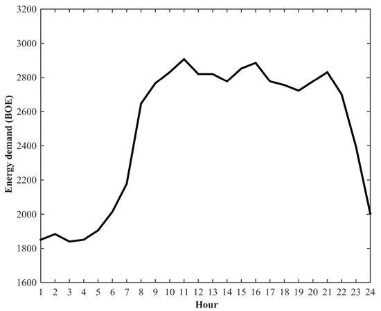
Figure 1. Energy demand profile.

5.2.1. Objective Function and Constraints

In the present study, the objective function for solving the EC problem is considered to reduce the cost of supplying energy demand. This objective function for 24-h study period is expressed by Equation (22). Additionally, to optimize the EC’s objective function, the constraints related to the start-up cost of power plants and their authorized production range, specified in Equations (23)–(25), must be considered.

$$F_{objective}=min\{{{\displaystyle \sum }}_{t=1}^T[{{\displaystyle \sum }}_{i=1}^{N_c}carrie{r}_i^t\times pric{e}_i+{{\displaystyle \sum }}_{i=1}^{N_g}S{C}_i^t+{{\displaystyle \sum }}_{i=1}^{N_g}{C}_i{u}_i^t] \},$$

(22)

$$S{C}_i^t=\{\begin{array}{cc}\hfill S{C}_i, & u_i^t>u_i^{t-1}\hfill \\ \hfill 0, & else\hfill \end{array},$$

(23)

$$P_{g_i}^{min}\le P_{g_i}\le P_{g_i}^{max},$$

(24)

$${{\displaystyle \sum }}_{i=1}^{N_g}{P}_{g_i}^t=loa{d}^t.$$

(25)

5.2.2. DPO Implementation to EC Problem

The purpose of implementing the EC problem is to supply energy demand by determining the most appropriate use of energy carriers, considering technical and economical constraints. In the study of each hour of the 24-h period the first step, after the required energy conversions, was to determine possible combinations of power plants based on the required electrical energy demand. Therefore, all possible combinations of power plants are determined for each hour of the study period. The second step involved determining a suitable pattern for energy carrier use for the entire study period, as well as the optimal combination of power plants for each hour, based on the objective function and using the proposed optimization algorithm. This convenient pattern of energy carrier usage is actually the main output of EC problem.

The EC problem is coded in MATLAB and executed on a system with a quad-core 3.3 GHz processor and 8 GB of RAM. The pseudo code of EC problem solution using DPO is specified in Algorithm 2.

Algorithm 2. DPO implementation to EC problem
START
1:	Problem information.
2:	Inputs data: $E_1^{study period }$, $T_{1,2}$
3:	For Hour = 1: Study period (24 h)
4:		$E_1=E_1^{study period }\left(\mathrm{Hour},:\right)$.
5:		$E_2$ calculation based (13).
6:		$E_3$ calculation based (14).
7:		$E_e= E_3\left(ed,1\right)$ and $ed$ = row number of electrical demand in $E_3$.
8:	END Hour
9:	Determine possible combinations of power plants for electrical demand supplying.
10:	DPO
11:	Initial population formation based on possible combinations of units.
12:		ITERATION = 1:T
13:			For i = 1:Npopulatio
14:				Combination = population (i,:).
15:					IF this combination is possible.
16:						UC Problem solving.
17:							input energy to power plants calculation.
18:						END UC solving.
19:							$E_4$ calculation based (15) to (18).
20:							Refinery simulation based (19).
21:							$E_5$ calculation based (20).
22:							$E_6$ calculation based (21).
23:							Fitness calculation based (22).
24:					Else if the combination is impossible.
25:							Fitness = 1 × 10.
26:					END if
27:			END FOR
28:			Updating $f_{worst}$ and $P_{worst}$ based (4).
29:			Updating $f_{best}$ and $P_{best}$ based (5).
30:			Updating based (3).
31:			FOR i = 1:N
32:				Updating $dosag{e}_i$ based (2).
33:				Updating $P_i$ based phase a. (6) and (7).
34:				Updating $P_i$ based phase b. (8) and (9).
35:				Updating $P_i$ based phase c. (10).
36:			END FOR
37:		END ITERATION
38:	EC outputs (for every hour and whole period of study).
39:		Determining the pattern of energy carriers using.
40:		Determining the UC output (power plant production).
41:		Convergence curve.
42:		Cost of energy supply.
43:		Import and export of energy carriers.
END

5.2.3. Results and Discussion

The proposed DPO algorithm was implemented on the power system in order to achieve optimal results in an economical manner for the introduced energy commitment problem. The purpose of this operation is to reduce operating costs in order to supply energy demand. The important output of the energy commitment problem, the determination of the amount of different energy carriers for each hour of the study period, is specified in Table 5. The convergence curve (as an important indicator in the evaluation of optimization algorithms) of the implementation of the DPO on the EC problem is drawn in Figure 2. This curve shows the precise behavior of the algorithm while reaching the appropriate response, indicating the exploitation, exploration and power of the proposed algorithm. Another important output of the EC is to determine the appropriate pattern for the on and off state of power plant units for each hour of period of study to supply the electrical demand which is specified in Table 6. Additionally, the hourly production rate of the units during the study period, the output of the UC problem, is presented in Table 7. Finally, the import and export values of the energy carriers based on domestic production are specified in Table 8. According to this table, Petroleum (399,217), Fuel oil (29,054.3), Gas oil (478.824), Kerosene (297.468), and Coke gas (92.2559) are in the export section and liquid gas (2451.409), Gasoline (20,384.46), plane fuel (2934.952), natural gas (12,502.36), and coal (906.6509) are in the import section.

Table 5. The need of energy carriers (BOE).

Hour	1	2	3	4	5	6	7	8
Liquid Gas	292.5897	297.7531	290.8686	292.5897	301.1953	318.4065	344.2232	418.2312
Fuel Oil	1107.223	1133.425	1098.565	1114.323	1132.174	1206.242	1284.84	1520.263
Gas Oil	1931.791	1963.236	1921.292	1930.419	1997.848	2110.83	2310.59	2837.866
Kerosene	661.1897	672.8578	657.3004	661.1897	680.6365	719.53	777.8703	945.1124
Gasoline	1694.256	1724.155	1684.29	1694.256	1744.087	1843.75	1993.243	2421.79
Plane Fuel	90.86539	92.4689	90.33089	90.86539	93.5379	98.88293	106.9005	129.8841
Natural Gas	7559.858	7691.954	7515.844	7564.33	7822.283	8285.097	9021.851	11,060.32
Coke Gas	45.5543	46.3582	45.28633	45.5543	46.89413	49.5738	53.59329	65.11585
Coal	100.6855	102.4623	100.0932	100.6855	103.6468	109.5695	118.4535	143.921
Hour	9	10	11	12	13	14	15	16
Liquid Gas	437.1635	447.4902	459.538	445.7691	445.7691	438.8846	450.9324	456.0957
Fuel Oil	1603.173	1653.536	1693.215	1651.406	1649.966	1612.975	1662.116	1685.183
Gas Oil	2960.847	3026.316	3117.653	3013.492	3013.89	2971.341	3054.712	3091.246
Kerosene	987.8952	1011.231	1038.457	1007.342	1007.342	991.7846	1019.01	1030.678
Gasoline	2531.418	2591.216	2660.979	2581.249	2581.249	2541.385	2611.148	2641.047
Plane Fuel	135.7636	138.9706	142.7121	138.4361	138.4361	136.2981	140.0396	141.6431
Natural Gas	11,593.93	11,881.31	12249.3	11,829.5	11,829.94	11,641.09	11982.27	12134.19
Coke Gas	68.06348	69.67128	71.54705	69.40331	69.40331	68.33145	70.20721	71.01111
Coal	150.4359	153.9895	158.1354	153.3973	153.3973	151.0282	155.1741	156.9509
Hour	17	18	19	20	21	22	23	24
Liquid Gas	438.8846	435.4424	430.279	438.8846	447.4902	426.8368	378.6455	316.6853
Fuel Oil	1614.772	1593.371	1563.759	1619.075	1654.976	1550.461	1418.204	1209.212
Gas Oil	2969.852	2950.352	2918.868	2967.727	3025.918	2894.268	2530.552	2097.053
Kerosene	991.7846	984.0059	972.3378	991.7846	1011.231	964.5591	855.6573	715.6406
Gasoline	2541.385	2521.452	2491.554	2541.385	2591.216	2471.621	2192.567	1833.783
Plane Fuel	136.2981	135.2291	133.6256	136.2981	138.9706	132.5566	117.5905	98.34843
Natural Gas	11,638.75	11,546.77	11,404.7	11,636.14	11,880.87	11,306.04	9885.869	8211.221
Coke Gas	68.33145	67.79552	66.99162	68.33145	69.67128	66.45568	58.95262	49.30583
Coal	151.0282	149.8437	148.0669	151.0282	153.9895	146.8823	130.2988	108.9772

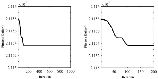
Figure 2. Convergence curve of doctor and patient optimization (DPO) on energy commitment (EC) solving.

Table 6. Appropriate combination of units and total cost for energy supply.

Hour	1	2	3	4	5	6	7	8	9	10	11	12	Cost ($)
Combination	10	10	10	11	13	17	19	22	23	22	26	22
Hour	13	14	15	16	17	18	19	20	21	22	23	24	2.1153 × 107
Combination	21	23	22	24	20	23	22	18	22	17	15	12

Table 7. Unit commitment (UC) result (MW).

Hour	unit 1	Unit 2	unit 3	unit 4	unit 5	unit 6	unit 7	unit 8	unit 9	unit 10	unit 11	unit 12	unit 13
1	400	400	350	197	197	197	65.66526	54.25	54.25	54.25	0	0	0
2	400	400	350	197	197	197	100.4196	54.25	54.25	54.25	0	0	0
3	400	400	350	197	197	196.8305	54.25	54.25	54.25	54.25	0	0	0
4	400	400	350	197	197	183.4153	54.25	54.25	54.25	54.25	25	0	0
5	400	400	350	197	197	191.3392	54.25	54.25	54.25	54.25	25	25	25
6	400	400	350	197	197	197	103.6372	54.25	54.25	54.25	25	25	25
7	400	400	350	197	197	197	155	155	67.90913	54.25	25	25	25
8	400	400	350	197	197	197	155	155	155	155	100	100	100
9	400	400	350	197	197	197	155	155	155	155	100	100	100
10	400	400	350	197	197	197	155	155	155	155	100	100	100
11	400	400	350	197	197	197	155	155	155	155	100	100	100
12	400	400	350	197	197	197	155	155	155	155	100	100	100
13	400	400	350	197	197	197	155	155	155	155	100	100	100
14	400	400	350	197	197	197	155	155	155	155	100	100	100
15	400	400	350	197	197	197	155	155	155	155	100	100	100
16	400	400	350	197	197	197	155	155	155	155	100	100	100
17	400	400	350	197	197	197	155	155	155	155	100	100	100
18	400	400	350	197	197	197	155	155	155	155	100	100	100
19	400	400	350	197	197	197	155	155	155	155	100	100	100
20	400	400	350	197	197	197	155	155	155	155	100	100	100
21	400	400	350	197	197	197	155	155	155	155	100	100	100
22	400	400	350	197	197	197	155	155	155	155	100	100	100
23	400	400	350	197	197	197	155	155	155	155	100	32.25505	25
24	400	400	350	197	197	197	155	77.1024	54.25	54.25	25	25	0
Hour	unit 14	unit 15	unit 16	unit 17	unit 18	unit 19	unit 20	unit 21	unit 22	unit 23	unit 24	unit 25	unit 26
1	0	0	0	0	0	0	0	0	0	0	0	0	0
2	0	0	0	0	0	0	0	0	0	0	0	0	0
3	0	0	0	0	0	0	0	0	0	0	0	0	0
4	0	0	0	0	0	0	0	0	0	0	0	0	0
5	0	0	0	0	0	0	0	0	0	0	0	0	0
6	15.2	15.2	15.2	15.2	0	0	0	0	0	0	0	0	0
7	15.2	15.2	15.2	15.2	4	4	0	0	0	0	0	0	0
8	76	29.30535	15.2	15.2	4	4	4	4	2.4	0	0	0	0
9	76	76	76	32.7381	4	4	4	4	2.4	2.4	0	0	0
10	76	76	76	76	20	19.04687	4	4	0	0	0	0	0
11	76	76	76	76	20	20	20	20	12	12	12	9.740442	2.4
12	76	76	76	76	20	5.062077	4	4	2.4	0	0	0	0
13	76	76	76	76	20	7.462077	4	4	0	0	0	0	0
14	76	76	76	44.32289	4	4	4	4	2.4	2.4	0	0	0
15	76	76	76	76	20	20	20	7.816464	2.4	0	0	0	0
16	76	76	76	76	20	20	20	20	12	10.57085	2.4	0	0
17	76	76	76	53.12289	4	4	4	0	0	0	0	0	0
18	76	76	76	21.1533	4	4	4	4	2.4	2.4	0	0	0
19	76	76	49.59892	15.2	4	4	4	4	2.4	0	0	0	0
20	76	76	76	61.12289	4	0	0	0	0	0	0	0	0
21	76	76	76	76	20	16.64687	4	4	2.4	0	0	0	0
22	76	76	44.82932	15.2	0	0	0	0	0	0	0	0	0
23	15.2	15.2	0	0	0	0	0	0	0	0	0	0	0
24	0	0	0	0	0	0	0	0	0	0	0	0	0

Table 8. Import and export of carriers (BOE).

Hour	Import	Export
Petroleum	0	−399,217
Liquid Gas	2451.409	0
Fuel Oil	0	−29,054.3
Gas Oil	0	−478.824
Kerosene	0	−297.468
Gasoline	20,384.46	0
Plane Fuel	29,34.952	0
Natural Gas	12,502.36	0
Coke Gas	0	−92.2559
Coal	906.6509	0

5.2.4. Comparison DPO and Other Algorithms on EC Problem

In order to evaluate the performance of the proposed algorithm in solving the EC, the other eight algorithms mentioned in this paper have been implemented on the EC problem. The results of this simulation are presented in Table 9. This table specifies the value of the objective function for each of the optimization algorithms. The proposed DPO algorithm is the best optimizer among the compared algorithms with the value of the objective function equal to 2.1153 × 10⁷ Dollar. WOA with the value of the objective function 2.1739 × 10⁷ Dollar, MPA with the value of the objective function 2.2365 × 10⁷ Dollar, GWO with the value of the objective function 2.4257 × 10⁷ Dollar, GOA with the value of the objective function 2.7592 × 10⁷ Dollar, TLBO with the value of the objective function 3.2648 × 10⁷ Dollar, GSA with the value of the objective function 6.7624 × 10⁷ Dollar, PSO with The value of the target function is 5.2158 × 10⁸ Dollar, and the GA with the value of the target function of 8.5146 × 10⁸ Dollar are ranked second to ninth, respectively. Based on the results, the proposed algorithm has a high ability to solve the EC problem and is much more competitive than the other eight algorithms.

Table 9. Results for DPO and other algorithms in EC problem.

Algorithm	Avg (Dollar)	Std (Dollar)	Rank
GA	8.5146$\times {10}^8$	2.6145$\times {10}^6$	9
PSO	5.2158$\times {10}^8$	1.2485$\times {10}^6$	8
GSA	6.7624$\times {10}^7$	5.2176$\times {10}^4$	7
TLBO	3.2648$\times {10}^7$	7.5423$\times {10}^3$	6
GOA	2.7592$\times {10}^7$	8.6427$\times {10}^2$	5
GWO	2.4257$\times {10}^7$	6.5654$\times {10}^2$	4
WOA	2.1739$\times {10}^7$	2.7865$\times {10}^2$	2
MPA	2.2365$\times {10}^7$	1.4552$\times {10}^2$	3
DPO	2.1153$\times {10}^7$	7.5142	1

6. Conclusions

A new doctor and patient optimization (DPO) Algorithm was introduced based on a simulation of the patient treatment process. This treatment process has three phases including vaccination, drug administration, and surgery. To evaluate the effectiveness and performance of the DPO, two case studies were considered. In case study A, the performance and effectiveness of the proposed DPO algorithm was evaluated on a benchmark standard test function with twenty-three objective functions and compared to eight other algorithms. These results show the exploitation and exploration capacity of the proposed algorithm in solving optimization problems. In case study B, the proposed DPO algorithm was implemented on the energy commitment (EC) problem in a power system with twenty-six power plants and various energy sectors, including residential, commercial, public, industrial, transportation, and agriculture sectors. The purpose of the EC was to determine the appropriate pattern of use of energy carriers to supply energy demand and minimize operation costs considering the technical constraints. The DPO with high exploitation and exploration capacity was well implemented on the EC problem, and its results were determined including the appropriate pattern of use of energy carriers, proper composition, and production of power plants, as well as the amount of import and export of energy carriers.

In future works, the authors propose several study ideas, such as solving the EC problem using other optimization algorithms and techniques, creating a binary variant of the DPO which has an important potential contribution, and applying DPO to overcome many-objective real-life optimization problems, as well as multi-objective problems.

References

- IEA. Energy Statistics Manual; OECD Publishing: Paris, France, 2004. [Google Scholar]
- Dehghani, M.; Montazeri, Z.; Ehsanifar, A.; Seifi, A.R.; Ebadi, J.M.; Grechko, O. Planning of energy carriers based on final energy consumption using dynamic programming and particle swarm optimization. Elec. Eng. Electromech. 2018, 5, 62–71. [Google Scholar] [CrossRef]
- Dehghani, M.; Montazeri, Z.; Malik, O. Energy commitment: A planning of energy carrier based on energy consumption. Электрoтехника и Электрoмеханика 2019, 6. [Google Scholar] [CrossRef]
- Smith, D.K.; Bertsekas, D.P. Nonlinear Programming. J. Oper. Res. Soc. 1997, 48, 334. [Google Scholar] [CrossRef]
- Bellman, R. Dynamic programming. Science 1966, 153, 34–37. [Google Scholar] [CrossRef] [PubMed]
- Frank, M.; Wolfe, P. An algorithm for quadratic programming. Nav. Res. Logist. Q. 1956, 3, 95–110. [Google Scholar] [CrossRef]
- Mirjalili, S.; Mirjalili, S.M.; Lewis, A. Grey Wolf Optimizer. Adv. Eng. Softw. 2013, 69, 46–61. [Google Scholar] [CrossRef]
- Yazdani, M.; Jolai, F. Lion Optimization Algorithm (LOA): A nature-inspired metaheuristic algorithm. J. Comput. Des. Eng. 2015, 3, 24–36. [Google Scholar] [CrossRef]
- Dorigo, M.; Stützle, T. Ant Colony Optimization: Overview and Recent Advances. Handb. Metaheuristics. Int. Ser. Oper. Res. Manag. Sci. 2019, 272, 311–351. [Google Scholar]
- Dehghani, M.; Mardaneh, M.; Malik, O.P.; NouraeiPour, S.M. DTO: Donkey Theorem Optimization. In Proceedings of the 2019 27th Iranian Conference on Electrical Engineering (ICEE), Yazd, Iran, 30 April–2 May 2019; Institute of Electrical and Electronics Engineers: New Jersey, NJ, USA, 2019; pp. 1855–1859. [Google Scholar]
- Barry, J.; Thron, C. A Computational Physics-Based Algorithm for Target Coverage Problems. In Advances in Nature-Inspired Computing and Applications; Shandilya, S., Nagar, A., Eds.; Springer: Cham, Germany, 2019; pp. 269–290. [Google Scholar]
- Dehghani, M.; Montazeri, Z.; Dehghani, A.; Seifi, A. Spring search algorithm: A new meta-heuristic optimization algorithm inspired by Hooke’s law. In Proceedings of the 4th International Conference on Knowledge-Based Engineering and Innovation (KBEI), Berlin, Germany, 21–23 December 2017; pp. 0210–0214. [Google Scholar]
- Eskandar, H.; Sadollah, A.; Bahreininejad, A.; Hamdi, M. Water cycle algorithm–A novel metaheuristic optimization method for solving constrained engineering optimization problems. Comput. Struct. 2012, 110, 151–166. [Google Scholar] [CrossRef]
- Rashedi, E.; Nezamabadi-Pour, H.; Saryazdi, S. GSA: A Gravitational Search Algorithm. Inf. Sci. 2009, 179, 2232–2248. [Google Scholar] [CrossRef]
- Kirkpatrick, S.; Gelatt, J.C.D.; Vecchi, M.P. Optimization by Simulated Annealing. World Sci. Lect. Notes Phys. 1986, 220, 339–348. [Google Scholar] [CrossRef]
- Moghaddam, F.F.; Moghaddam, R.F.; Cheriet, M. Curved space optimization: A random search based on general relativity theory. arXiv 2012, arXiv:1208.2214. [Google Scholar]
- Shah-Hosseini, H. Principal components analysis by the galaxy-based search algorithm: A novel metaheuristic for continuous optimisation. Int. J. Comput. Sci. Eng. 2011, 6, 132. [Google Scholar] [CrossRef]
- Alatas, B. ACROA: Artificial Chemical Reaction Optimization Algorithm for global optimization. Expert Syst. Appl. 2011, 38, 13170–13180. [Google Scholar] [CrossRef]
- Formato, R.A. Central Force Optimization: A New Nature Inspired Computational Framework for Multidimensional Search and Optimization. In Nature Inspired Cooperative Strategies for Optimization (NICSO 2007); Krasnogon, N., Nicosia, V., Pavone, M., Pelta, D.A., Eds.; Springer Science and Business Media LLC: Berlin, Germany, 2008; Volume 129, pp. 221–238. [Google Scholar]
- Du, H.; Wu, X.; Zhuang, J. Small-World Optimization Algorithm for Function Optimization. In Proceedings of the Computer Vision, Xi’an, China, 24–28 September 2006; Springer Science and Business Media LLC: Berlin, Germany, 2006; pp. 264–273. [Google Scholar]
- Bansal, J.C. Particle Swarm Optimization. In Evolutionary and Swarm Intelligence Algorithms; Springer Science and Business Media LLC: Berlin, Germany, 2018; pp. 11–23. [Google Scholar]
- Saremi, S.; Mirjalili, S.; Lewis, A. Grasshopper Optimisation Algorithm: Theory and application. Adv. Eng. Softw. 2017, 105, 30–47. [Google Scholar] [CrossRef]
- Faramarzi, A.; Heidarinejad, M.; Mirjalili, S.; Gandomi, A.H. Marine Predators Algorithm: A nature-inspired metaheuristic. Expert Syst. Appl. 2020, 152, 113377. [Google Scholar] [CrossRef]
- Gandomi, A.H.; Yang, X.-S.; Alavi, A.H. Cuckoo search algorithm: A metaheuristic approach to solve structural optimization problems. Eng. Comput. 2011, 29, 17–35. [Google Scholar] [CrossRef]
- Karaboga, D.; Basturk, B. Artificial Bee Colony (ABC) Optimization Algorithm for Solving Constrained Optimization Problems. Comput. Vis. 2007, 4529, 789–798. [Google Scholar] [CrossRef]
- Mirjalili, S. The Ant Lion Optimizer. Adv. Eng. Softw. 2015, 83, 80–98. [Google Scholar] [CrossRef]
- Mirjalili, S.; Lewis, A. The Whale Optimization Algorithm. Adv. Eng. Softw. 2016, 95, 51–67. [Google Scholar] [CrossRef]
- Yang, X.-S. A New Metaheuristic Bat-Inspired Algorithm. In Nature Inspired Cooperative Strategies for Optimization (NICSO 2010); Krasnogon, N., Nicosia, V., Pavone, M., Pelta, D.A., Eds.; Springer Science and Business Media LLC: Berlin, Germany, 2010; Volume 284, pp. 65–74. [Google Scholar]
- Castillo, O.; Aguilar, L.T. Genetic Algorithms. In Type-2 Fuzzy Logic. in Control. of Nonsmooth Systems; Springer: Cham, Switzerland, 2019; pp. 23–39. [Google Scholar]
- Beyer, H.-G.; Schwefel, H.-P. Evolution strategies—A comprehensive introduction. Nat. Comput. 2002, 1, 3–52. [Google Scholar] [CrossRef]
- Storn, R.; Price, K. Differential Evolution-A Simple and Efficient Adaptive Scheme for Global Optimization Over Continuous Spaces; Berkeley: Berkeley, CA, USA, 1995. [Google Scholar]
- Mirjalili, S. BiogeographyB-Based Optimisation. In Evolutionary Algorithms and Neural Networks; Krasnogon, N., Nicosia, V., Pavone, M., Pelta, D.A., Eds.; Springer Science and Business Media LLC: Berlin, Germany, 2018; pp. 57–72. [Google Scholar]
- Koza, J.R. Genetic programming: A Paradigm for Genetically Breeding Populations of Computer Programs to Solve Problems; Stanford University, Department of Computer Science: Stanford, CA, USA, 1990. [Google Scholar]
- Dehghani, M.; Montazeri, Z.; Malik, O.P. DGO: Dice Game Optimizer. Gazi Univ. J. Sci. 2019, 32, 871–882. [Google Scholar] [CrossRef]
- Dehghani, M.; Montazeri, Z.; Malik, O.P.; Ehsanifar, A.; Dehghani, A. 0OSA: Orientation Search Algorithm. Int. J. Ind. Elect. Control. Optim. 2019, 2, 99–112. [Google Scholar]
- Dehghani, M.; Shiraz University of Technology; Montazeri, Z.; Malik, O.; Givi, H.; Guerrero, J. University of Calgary; University of Shahreza; Aalborg University Shell Game Optimization: A Novel Game-Based Algorithm. Int. J. Intell. Eng. Syst. 2020, 13, 10. [Google Scholar] [CrossRef]
- Wood, A.J.; Wollenberg, B.F. Power Generation, Operation, and Control; John Wiley & Sons: New Jersey, NJ, USA, 2012. [Google Scholar]
- Abdou, I.; Tkiouat, M. Unit Commitment Problem in Electrical Power System: A Literature Review. Int. J. Electr. Comput. Eng. 2018, 8, 1357–1372. [Google Scholar] [CrossRef]
- Gögler, P.; Dorfner, M.; Hamacher, T. Hybrid Robust/Stochastic Unit Commitment With Iterative Partitions of the Continuous Uncertainty Set. Front. Energy Res. 2018, 6, 71. [Google Scholar] [CrossRef]
- Tiwari, S.; Dwivedi, B.; Dave, M. A two stage solution methodology for deterministic unit commitment problem. In Proceedings of the 2016 IEEE Uttar Pradesh Section International Conference on Electrical, Computer and Electronics Engineering (UPCON), Varanasi, India, 9–11 December 2016; pp. 317–322. [Google Scholar]
- Del Nozal, A.R.; Tapia, A.; Alvarado-Barrios, L.; Reina, D.G. Application of Genetic Algorithms for Unit Commitment and Economic Dispatch Problems in Microgrids. In Nature Inspired Computing for Data Science; Krasnogon, N., Nicosia, V., Pavone, M., Pelta, D.A., Eds.; Springer Science and Business Media LLC: Berlin, Germany, 2019; pp. 139–167. [Google Scholar]
- Gutiérrez-Alcaraz, G.; Hinojosa, V. Using Generalized Generation Distribution Factors in a MILP Model to Solve the Transmission-Constrained Unit Commitment Problem. Energies 2018, 11, 2232. [Google Scholar] [CrossRef]
- Hussein, B.M.; Jaber, A.S. Unit commitment based on modified firefly algorithm. Meas. Control. 2020, 53, 320–327. [Google Scholar] [CrossRef]
- Dhaliwal, J.S.; Dhillon, J.S. Profit based unit commitment using memetic binary differential evolution algorithm. Appl. Soft Comput. 2019, 81, 105502. [Google Scholar] [CrossRef]
- Nikzad, H.R.; Abdi, H. A robust unit commitment based on GA-PL strategy by applying TOAT and considering emission costs and energy storage systems. Electr. Power Syst. Res. 2020, 180, 106154. [Google Scholar] [CrossRef]
- Hussain, A.N.; Ismail, A.A. Operation cost reduction in unit commitment problem using improved quantum binary PSO algorithm. Int. J. Electr. Comput. Eng. 2020, 10, 1149–1155. [Google Scholar] [CrossRef]
- Strikanth, R.K.; Panwar, L.; Panigrahi, B.K.; Kumar, R. Binary whale optimization algorithm: A new metaheuristic approach for profit-based unit commitment problems in competitive electricity markets. Eng. Optim. 2018, 51, 369–389. [Google Scholar] [CrossRef]
- Panwar, L.K.; Reddy, S.; Verma, A.; Panigrahi, B.K.; Kumar, R. Binary Grey Wolf Optimizer for large scale unit commitment problem. Swarm Evol. Comput. 2018, 38, 251–266. [Google Scholar] [CrossRef]
- Ebrahimi, J.; Hosseinian, S.H.; Gharehpetian, G.B. Unit Commitment Problem Solution Using Shuffled Frog Leaping Algorithm. IEEE Trans. Power Syst. 2010, 26, 573–581. [Google Scholar] [CrossRef]
- Jo, K.-H.; Kim, M.-K. Improved Genetic Algorithm-Based Unit Commitment Considering Uncertainty Integration Method. Energies 2018, 11, 1387. [Google Scholar] [CrossRef]
- Simopoulos, D.; Kavatza, S.; Vournas, C. Reliability Constrained Unit Commitment Using Simulated Annealing. Ieee Trans. Power Syst. 2006, 21, 1699–1706. [Google Scholar] [CrossRef]
- Carrión, M.; Zarate-Minano, R.; Domínguez, R. A Practical Formulation for Ex-Ante Scheduling of Energy and Reserve in Renewable-Dominated Power Systems: Case Study of the Iberian Peninsula. Energies 2018, 11, 1939. [Google Scholar] [CrossRef]
- Li, J.; Niu, D.; Wu, M.; Wang, Y.; Li, F.; Dong, H. Research on Battery Energy Storage as Backup Power in the Operation Optimization of a Regional Integrated Energy System. Energies 2018, 11, 2990. [Google Scholar] [CrossRef]
- Dominković, D.F.; Stark, G.; Hodge, B.-M.; Pedersen, A.S. Integrated Energy Planning with a High Share of Variable Renewable Energy Sources for a Caribbean Island. Energies 2018, 11, 2193. [Google Scholar] [CrossRef]
- Kaur, S.; Awasthi, L.K.; Sangal, A.; Dhiman, G. Tunicate Swarm Algorithm: A new bio-inspired based metaheuristic paradigm for global optimization. Eng. Appl. Artif. Intell. 2020, 90, 103541. [Google Scholar] [CrossRef]
- Dhiman, G.; Garg, M.; Nagar, A.K.; Kumar, V.; Dehghani, M. A Novel Algorithm for Global Optimization: Rat Swarm Optimizer. J. Ambient Int. Human. Comp. 2020, 11, 1868–5145. [Google Scholar]
- Digalakis, J.; Margaritis, K.G. On benchmarking functions for genetic algorithms. Int. J. Comput. Math. 2001, 77, 481–506. [Google Scholar] [CrossRef]
- Wang, G.; Gandomi, A.H.; Yang, X.-S.; Alavi, A.H. A novel improved accelerated particle swarm optimization algorithm for global numerical optimization. Eng. Comput. 2014, 31, 1198–1220. [Google Scholar] [CrossRef]
- Yang, X.-S. Firefly algorithm, stochastic test functions and design optimisation. Int. J. Bio-Inspired Comput. 2010, 2, 78. [Google Scholar] [CrossRef]
- Mirjalili, S. Genetic Algorithm. In Evolutionary Algorithms and Neural Networks; Krasnogon, N., Nicosia, V., Pavone, M., Pelta, D.A., Eds.; Springer: Berlin, Germany, 2019; pp. 43–55. [Google Scholar]
- Mirjalili, S. Optimisation. In Evolutionary Algorithms and Neural Networks; Krasnogon, N., Nicosia, V., Pavone, M., Pelta, D.A., Eds.; Springer: Berlin, Germany, 2019; pp. 15–31. [Google Scholar]
- Rao, R.V.; Savsani, V.J.; Vakharia, D. Teaching–learning-based optimization: A novel method for constrained mechanical design optimization problems. Comput. Des. 2011, 43, 303–315. [Google Scholar] [CrossRef]
- Birol, F. International Energy Agency. Global Energy Review Report; IEA: Paris, France, 2004; pp. 1–50. [Google Scholar]
- U.S. Energy Information Administration (EIA). Available online: http://www.eia.gov (accessed on 12 August 2020).
© 2020 by the authors. Licensee MDPI, Basel, Switzerland. This article is an open access article distributed under the terms and conditions of the Creative Commons Attribution (CC BY) license (http://creativecommons.org/licenses/by/4.0/).