Using Machine Learning and Candlestick Patterns to Predict the Outcomes of American Football Games

Abstract

Match outcome prediction is a challenging problem that has led to the recent rise in machine learning being adopted and receiving significant interest from researchers in data science and sports. This study explores predictability in match outcomes using machine learning and candlestick charts, which have been used for stock market technical analysis. We compile candlestick charts based on betting market data and consider the character of the candlestick charts as features in our predictive model rather than the performance indicators used in the technical and tactical analysis in most studies. The predictions are investigated as two types of problems, namely, the classification of wins and losses and the regression of the winning/losing margin. Both are examined using various methods of machine learning, such as ensemble learning, support vector machines and neural networks. The effectiveness of our proposed approach is evaluated with a dataset of 13261 instances over 32 seasons in the National Football League. The results reveal that the random subspace method for regression achieves the best accuracy rate of 68.4%. The candlestick charts of betting market data can enable promising results of match outcome prediction based on pattern recognition by machine learning, without limitations regarding the specific knowledge required for various kinds of sports.

1. Introduction

Many people focus their attention on the outcomes of sports events. A match result has a significant impact on players, coaches, sports fans, journalists and bookmakers. Thus, many people attempt to predict match results before games. In recent years, detailed data gathered during games and the box scores of every competition in various sports have been systematically recorded and stored in databases. Given the vigorous development of machine learning technology, these databases have gradually gained attention, and classic sports analysis and prediction, such as technical and tactical analysis, offensive/defensive strategy analysis and opponent scouting, have extended to the field of the application of big data.

Many historical game performances of teams and players, as well as a wide variety of game-related data, have been used as a feed for machine learning modelling to enable prediction. However, the tournament systems, competition rules and point scoring systems of the various competitions are different. Thus, the indicators used to measure performance are different. The process of extracting characteristics to represent competition data is a challenge. Applying machine learning modelling and different data processing methods to various sports leads to different predicting accuracies. The adaptability of machine learning for predicting the outcome of a given sports competition is an important research topic.

This study proposes the use of candlestick charts and machine learning to predict the outcome of sports matches. Candlestick charts have been applied to financial market analysis for decades. The pattern of candlestick charts has been empirically proven to reveal adequately the behaviour of finance and is highly suitable for use in conjunction with machine learning in predicting the price fluctuations of financial commodities. As with the stock market, various analyses, such as fundamental, chip and technical analyses, exist. For sports competitions, this study’s innovative proposal was to borrow the technical analysis of the stock market and use candlesticks instead of indicators of sports performance to make predictions.

The purpose of this study is to present a methodology that combines the points scored and the odds of the betting market to create a candlestick chart of a sports tournament. The study also aims to extract the characteristics of machine learning modelling to predict match outcomes. To explore the feasibility of our proposed classification and regression approaches based on machine learning, data from a professional American football league (i.e., the National Football League, NFL) are used as empirical evidence. Only a few studies with weak prediction accuracy are available as reference.

The main contributions to the literature are as follows. First, we develop a consistent approach that incorporates candlestick charts and machine learning for sports predictions without domain knowledge in various sports. Second, we explore the impact of various candlestick features on the predicted outcomes. Third, we compare the different approaches of machine learning models to reveal which one can provide a more precise prediction. Fourth, we analyse in detail the differences in the predictions between teams and between home and away teams.

The rest of this paper is structured as follows. Section 2 contains an overview of related work. Section 3 describes the dataset, proposed methodology and experimental design. Section 4 conducts a performance analysis. Section 5 provides the concluding remarks and an outlook on our future work.

2. Related Work

2.1. Sports Forecasting and Machine Learning

Based on previous research, methods of predicting the outcomes of matches can be divided into two categories: namely, result-based and goal-based approaches. Result-based approaches aim to predict the result class, whereas goal-based approaches aim to predict the goals scored by each team in a certain match. In this context, predicting the winner and loser involves two approaches. Result-based approaches are usually conducted using classification-based models, where the predicted outcome is a categorical variable, such as win, loss or draw. Goal-based approaches are achieved using regression-based models, where the predicted outcome is a numerical variable of a score or a difference in score from that of the opponent, and the score is used to ascertain win, loss or draw. Other approaches can be used to predict the outcome of a match, such as using the probability distributions model to estimate win probability [1,2] or rating teams based on past performance and then predicting based on rankings [3,4,5].

Regardless of whether the model is classification–based or regression-based, the data used to construct the model are mostly performance indicators, which are usually retrieved and calculated from the offensive and defensive records of each team or each player. These performance indicators produced on a statistical basis have been explored in many studies in various sports [6,7], and are often used to predict the outcome of the game [8,9,10] and obtain explainable results.

In addition to using performance indicators, situation variables, also known as conditional factors, have been considered in many studies. Situational variables, such as match location, who scores first and the quality of the opponent, can potentially affect the structure of a match and eventually the outcome of the match; evidence has been presented to support the idea that situational variables are worth including when analysing performance from a behavioural perspective [11,12]. Moreover, a play’s position in the field is commonly considered in basketball [13,14] and football studies [9]. Additionally, in international competitions among different national teams, the gross domestic production per capita, population size and other relevant factors for each country have been considered [15,16].

Sarmento et al. [17] systematically reviewed the variables commonly used in many football match analysis studies and recommended the adoption of methodologies that include the general description of technical, tactical, physical performance, situational, continuous and sequential aspects of the game to make the science of match analysis easy to apply in the field. Studies have considered many variables to increase the complexity of the model. For example, Carpita et al. [9] used 33 player-related variables, seven player performance indicators and the position of a player or a role. The explosion of a large amount of input data accompanied by many variables has caused the traditional approach based on the statistical model to have many dimensions. Thus, many studies have instead used machine learning to process a large amount of data to construct black-box prediction models.

Utilising machine learning for predictive analysis has been studied in various sports tournaments [18], such as basketball [19,20,21], baseball [22], cricket [23], ice hockey [24] and football [25,26]. Many kinds of machine learning methods, such as artificial neural networks (ANNs), support vector machines (SVMs), random subspace (RS), random forests (RFs) and hybrid modelling approaches combining multiple methods, have been developed and used for comparison in match result prediction.

2.2. Candlestick Charts and Machine Learning

Candlestick charting can be traced back to the Japanese rice trades and financial instruments from centuries ago. It is a method for visualising data in different ways to predict recent stock price fluctuations and provide insights into market psychology. Japanese candlestick theory has become one of the most widely used technical analysis techniques for making investment decisions based on empirical finances. Future trends in financial time series are considered to be predictable by identifying specific candlestick patterns.

Some scholars have proposed ways to describe these known patterns with ordered fuzzy numbers [27] or formal specifications [28] to provide recognition using machine learning. Some scholars have characterised financial time series with candlestick charts and then used ANN, fuzzy logic, genetic algorithms, decision trees and various hybrid approaches to provide predictions about the market trend for investment decision use [29,30]. Given that candlestick charts incorporating machine learning have been beneficial in the application of finance, some studies in other fields have initiated applying them as a tool for analysis and prediction. They have been applied in studies on predicting teens’ stress level change on a micro-blog platform [31] and in sports metrics [32] to forecast game outcomes.

However, the application of candlestick charts in other fields is slightly beyond the applicability of the original financial time series. They need to be adjusted and modified to accommodate specific characteristics of the field. Whether candlestick charts exhibit certain patterns and corresponding behaviours as in the financial field and whether they are equally suitable for pattern recognition using machine learning to provide predictions are research areas to be examined.

2.3. Sports Forecasting in Betting Market

Betting on the sports market can be done in different ways. Regarding NFL games, Las Vegas sports bookmakers provide two bets, namely, the point spread (side bet) between each pair of teams and the total number of points scored by each pair of teams (over/under bet). Oddsmakers set the numbers (lines) for these two bets by creating a margin between the two teams. The point spread (or betting line) can be thought of as the betting market’s estimate of the difference between the points scored by each team. If a gambler bets on the favourite, he or she wins the bet if the favourite wins by more than the point spread. If a gambler bets on the underdog, he or she wins the bet if the underdog either wins or loses by less than the point spread.

The betting market has many similar characteristics to financial markets [33]. Sports bookmakers try to set their lines to ensure that an equal amount of money is bet on either side of the line. However, if new information is received that changes the outlook of the match or if bettors tend to favour one side of the line, then odds makers may change the line in the time leading up to the match to regain the desired balance of bets. In terms of the phenomenon of commodity prices in the financial market reflected in the efficient market hypothesis, the same phenomenon can be seen in the odds of the betting market. Balancing the bets on either side of the line is not always possible. Thus, the research issue is whether any predictable pattern in the betting lines exists over the preceding week [34].

Bookmakers’ odds are implicit representations of all kinds of information, including the past performance of players and teams, a mix of instant and asynchronous messages and a wide variety of components of sports fan psychology; current stock prices reflect all information rationally and instantaneously to the market in three forms, namely, weak, semi-strong and strong [35]. Moreover, the random walk behaviour exhibited by stock price fluctuations makes the profit forecasting models non-persistent for a long time, which can also be observed in the betting market. Although profit forecasting models exist in the financial and betting markets during periods of market inefficiency [36], extensive modelling innovations are required [37].

Many studies have recommended utilising betting market data released by bookmakers in predictive models [38,39,40]. The results demonstrate that betting odds and margins have a rather high predictive accuracy, which is justified because bookmakers cannot survive on inefficient odds and margins. Thus, bookmakers’ predictions implied from the odds have often been used as a comparison group in studies on match outcome prediction. Consequently, we suggest that betting markets should also be relevant to the principles of stock market technical analysis. The historical data of the betting market can be manipulated to draw candlestick charts to identify the features of the matches and used for machine learning modelling to develop predictive models.

2.4. Analysis and Prediction of American Football

American football, such as NFL games, operates with a highly complex scoring system, making it highly demanding to model the points scored using standard modelling approaches. NFL players can score in five ways: an unconverted touchdown (six points), a touchdown with a one-point conversion (seven points), a touchdown with a two-point conversion (eight points), a safety (two points) or a field goal (three points). Other sports, such as football, baseball and basketball, follow relatively simple rules for giving scores under limited conditions. Consequently, American football predictions are highly challenging, regardless of whether traditional statistical models, modern machine learning models or even bookmakers’ predictions are used, with lower accuracy than in other sports. However, this challenge reveals opportunities for improvement in prediction models, leading to many studies being devoted to it.

Song et al. [41] compared the prediction of the outcomes of NFL games by experts, statistical models and opening betting lines on two NFL seasons. The findings showed that the distinctions between experts and statistical systems in predicting the accuracy of contest winners were not statistically significant and that betting lines performed better than the other two. David et al. [42] analysed the ability of a neural network model to predict the outcome of NFL games. This model only adopted readily available statistics, such as rushing yards, passing yards, fumbles lost and scoring, and proposed the inclusion of differences in statistics between teams for comparison. Baker and McHale [43] presented a point process model for forecasting end-of-match exact scores in NFL games. Historical tournament information, including the teams’ scores, the field of play, records for each game, various game statistics and data given by bookmakers, such as the margin (point spread) and the over/under for each game, was obtained for the study. With a set of simple covariates based on past match statistics, the model performed as well as bookmakers in predicting match outcomes and exact scores. Pelechrinis and Papalexakis [44] collected play-by-play data from the past seven seasons of the NFL and built a descriptive model for the probability of the home team winning a game. A football prediction matchup engine was provided by combining this descriptive model with a statistical bootstrap module. It achieved an overall accuracy of 63.4%, which outperformed the baseline prediction based on win-loss standings every season. Schumaker et al. [45] examined the application of techniques from technical charting used in stock price analysis to sentiment gathered from social media for NFL game outcome prediction. The sentiment polarity was analysed as a time-series signal, examining the position and magnitude of signal change between two temporal windows. The 50- and 200-day moving averages, which are popular techniques to analyse price movements in stock technical charts, can be adopted to find patterns, such as golden and death crosses.

These NFL outcome prediction studies have employed different variables and methods. The experiments within them were designed and measured in different ways. They used different datasets to ensure that the criteria for accuracy were calculated differently and were not easy to compare. However, most studies have compared their models with betting market predictions; some models were better, and some were worse. Therefore, we suggest the use of interdisciplinary predictive models that combine stock market technical analysis, betting market behaviour, sports prediction and machine learning in data science. They have the potential to improve on previous approaches and lead to a new research direction.

3. Methodology

3.1. Data Transformation into Candlestick

Candlestick charts used for sports outcome analysis are plotted based on the odds of the sports betting market and the relative actual match outcome. Each candlestick represents a game. The line on winning/losing margin between the team and its opponent (denoted as LD), the line on the total points scored by both teams (denoted as LT), the actual margin (denoted as D) and the actual total points scored (denoted as T) are gathered as the raw data for each game to plot the candlestick.

In general, a candlestick in the stock market is defined by the open-high-low-close (OHLC) price, as shown in Figure 1a. In the sports betting market, we refer to Malios’s method [32] and take LD as “open” and D as “close”. The gambling shock reflecting the gap between expectation and reality is defined as the difference between a game outcome and its corresponding line. The difference between “open” and “close” is treated as the gambling shock related to the line on the winning/losing margin between the team and its opponent, denoted as GSD. GSD is similar to the price spread in the stock market and forms the candlestick’s body length. The difference between LT and T is treated as the gambling shock related to the line on the total points scored by both teams, denoted as GST. GST is similar to the intraday price fluctuation degree in the stock market and forms the candlestick’s wick length. If GST > 0, the wick extends above the body. If GST < 0, the wick extends below the body. If GST = 0, no wick exists. In general, the wick is called the shadow, and the lower wick is called the tail. The candlestick’s body colour is dependent on the relationship of D and LD. If D > LD, the body colour is white, and the body’s maximum and minimum values are defined by D and LD. If LD > D, the body colour is black, and the body’s maximum and minimum values are defined by LD and D. Figure 1b illustrates the use of the candlestick chart in this study. The notations and definitions are as follows:

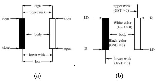
Figure 1. Candlestick. (a) Stock market data; (b) Sports data. The difference between “open” and “close” is treated as the gambling shock related to the line on the winning/losing margin between the team and its opponent, denoted as GSD; The difference between LT (the line on the total points scored by both teams) and T (the actual total points scored) is treated as the gambling shock related to the line on the total points scored by both teams, denoted as GST.

• D: Team winning/losing margin (i.e., the difference in points scored between the team and its opponent)
• LD: Line (or spread) on the winning/losing margin between the team and its opponent; the side line in the betting market
• T: Total points scored by both teams
• LT: Line on the total points scored by both teams; the over/under (O/U) line in the betting market

  $$\mathrm{GSD}=\mathrm{D}-\mathrm{LD}$$

  (1)

  $$\mathrm{GST}=\mathrm{T}-\mathrm{LT}$$

  (2)

In this study, we redefine D by calculating the points scored by the opponent team minus the points scored by the favourite team. The opposite value differs according to the value proposed by Mallios. However, by this modification, winning/losing based on the negative/positive value of D and LD becomes consistent. For example, when LD is −5.5, the favourite team wins and may exceed the opposing team’s score by 5.5 points. In other words, if the value of LD is negative, the favourite team wins; if it is positive, the favourite team loses. Using this method would reflect the gambling shock appropriately. Finally, the candlestick chart defined by OHLC and the body colour are formulated as follows:

$$\mathrm{O}=\mathrm{LD}$$

(3)

$$\mathrm{H}=\{\begin{array}{l}\mathrm{MAX}(\mathrm{D},\mathrm{LD})+\mathrm{GST}(\mathrm{if}\mathrm{GST}>0)\\ \mathrm{MAX}(\mathrm{D},\mathrm{LD})(\mathrm{if}\mathrm{GST}<0)\end{array}$$

(4)

$$\mathrm{L}=\{\begin{array}{l}\mathrm{MIN}(\mathrm{D},\mathrm{LD})(\mathrm{if}\mathrm{GST}>0)\\ \mathrm{MIN}(\mathrm{D},\mathrm{LD})-\mathrm{GST}(\mathrm{if}\mathrm{GST}<0)\end{array}$$

(5)

$$\mathrm{C}=\mathrm{D}$$

(6)

$$\mathrm{Body}\mathrm{color}=\{\begin{array}{l}\mathrm{White}(\mathrm{if}\mathrm{D}>\mathrm{LD})\\ \mathrm{Black}(\mathrm{if}\mathrm{LD}>\mathrm{D})\end{array}$$

(7)

Seattle’s candlestick chart during the 2012–2013 and 2013–2014 seasons, including the pre-season, regular season, and post-season, is plotted in Figure 2 as an example.

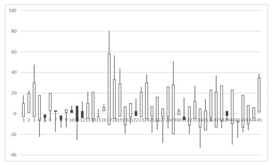
Figure 2. Seattle’s candlestick chart in 2012/2013 and 2013/2014.

Some differences can observed between the candlestick charts for sports betting and stock prices. First, the value of the stock price must be positive to ensure that the corresponding candlesticks remain positive. However, the outcome of a game is either losing or winning. Thus, the corresponding candlesticks can be positive or negative. Second, the typology of a stock candlestick is diversification, but the appearance of a sports candlestick is limited. Sports candlesticks lack the type with the upper and lower wick. Third, for stock candlesticks, the colour of a candlestick is consistent with the price difference at opening and closing, and the stock price is up or down. However, the colour of the sports candlestick is derived from the opening and closing differences but does not necessarily represent winning or losing. Although the information covered by the sports candlestick chart is not as much as that of the stock candlestick chart, the volatility of betting odds and the relationship of the time series can also be graphically presented to provide another perspective and reference for analysts.

3.2. Feature Engineering and Selection

Regarding the fluctuations and predictions in stock prices in the financial market, we can make a candlestick chart for sports, which reflects the time series of fluctuations in betting odds and actual scores, and predict the results of sports games. How to describe the changes in these fluctuations and extract the relevant characteristics is an issue to be investigated by this study.

We refer to some stock technique analysis concepts and use the following types of indicators as characteristics of candlesticks. (a) OHLC: the OHLC sequence and its colour make up the candlestick chart. (b) Length: the mean size of the candlestick’s body and wick includes the length of the body and upper and lower wick. (c) Length style: the categories of length are very short, short, zero, long and very long. (d) Relation style: the categories based on the relationship compared with the previous candlestick are low, equal low, equal, equal high and high. This style is applied to describe the related position of the open and close of the candlestick, referred to as the open style and close style. (e) Time series: a series of variables indexed in time order. A variable denoted by V and the time series at data points t − 2, t − 1 and t are expressed as V (t − 2), V (t − 1) and V (t), respectively.

When dealing with the length values of the body and wick, the maximum value of the margin and the total score of the game can be found in previous game records, and the minimum value is zero. Thus, we make the numerical scale of length consistent by min-max normalising to between 0 and 1 and then converting the length to a categorical variable, referred to as length style, depending on the degree. The original value of the length, the normalised value of the length and the length style are selected as features. However, special instances of zero length occur in many cases, such as a zero upper wick and a zero lower wick, which cause the issue of imbalanced data in machine learning. To address this issue, we specifically treat “zero” as a separate category of length style.

In this study, the length and relationship between adjacent candlesticks can be transformed into categorical variables to become length, open and close styles, mainly considering the expression of the candlestick pattern. The pattern of candlesticks can be expressed in several ways. Some studies have used the exact threshold value to express the relationship with the previous candle as a percentage [28]. Some studies have expressed it in the form of fuzzy variables for fuzzy inference [29,46]. Given that the pattern of the sports candlestick chart is unknown, it cannot be recognised by fuzzy inference. However, we can still use fuzzy linguistic variables to characterise the features of the candlestick chart appropriately, converting the numerical values into categories by setting the membership function. Figure 3 illustrates the membership function of the linguistic variables for length style, which represents the degree of the candlestick’s body or wick length. The x-axis in the figure indicates the length of the body or wick on a normalised scale from 0 to 1. The categories of very long and very short on both sides of the figure are defined by the linear membership function, and the categories of short and long in the centre of the figure are defined by the triangle function.

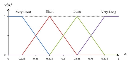
Figure 3. Membership function of the linguistic variables for length style.

The candlestick patterns also include the characteristics of trends. The consequent trend of the candlestick is measured by the relationship between two adjacent candlesticks. Comparing the current candlestick with the previous one, the relative position of the open and close, referred to as open style and close style, is used to indicate the trend. Five linguistic variables, namely, low, equal low, equal, equal high, and high, are defined to represent the open and close style. Figure 4 shows the membership function of these linguistic variables. The previous candlestick is plotted at the bottom of the figure for comparison. The locations of the five linguistic variables are plotted according to the previous candlestick as shown in the figure. The position of open/close for the current candlestick is located by its numerical value on the x-axis, and the relation style is determined according to the y-axis, which gives the possible value of the membership function.

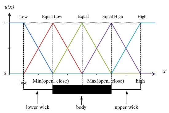
Figure 4. Membership function of the linguistic variables for open and close styles.

To capture the features of continuous time variation in the candlestick chart, we treated specific features as time series and considered their data points in antecedent and posterior time simultaneously as input variables for the predictive model. The candlestick chart of the stock market’s daily trading data shows the two- and three-day trading patterns presented by two and three successive candlesticks, respectively. For example, the well-known engulfing pattern is presented by two successive candlesticks, which suggest a potential trend reversal. The first candlestick has a small body that is completely engulfed by the second candlestick. It is referred to as a bullish engulfing pattern when it appears at the end of a downtrend and a bearish engulfing pattern when it appears after an uptrend. Another example is the well-known evening star, which is a bearish reversal pattern presented by three successive candlesticks. The first candlestick continues the uptrend. The second candlestick gaps up and has a narrow body. The third candlestick closes below the midpoint of the first candlestick. As a result, three consecutive candlesticks, V (t − 2), V (t − 1) and V (t), can be used as variables to predict the outcome of the next game at t + 1.

In conjunction with the above features of the candlestick, the field of the match in the situation variable is adopted as a feature because it potentially affects the outcome of a match, such as home advantage [47,48,49]. Moreover, the pre-game odds are considered as an important variable. Given that the pre-game odds have already implied the predictions in bookmakers’ betting on the outcome of the match, forecasting the outcome based on the odds and their volatility trend is an innovation. Finally, all of the features selected as variables for the prediction model in this study are summarised in Table 1. A total of 46 features corresponding to two different output variables can be selected to build the classification-based and regression-based models.

Table 1. Description of the features used in this study.

Notation	Description	Categories
PS	Point score	Game result
PA	Point allow	Game result
TP	Total points scored	Game result
Field	Match field, such as home or away	Situation variable
Outcome	Outcome, such as win or lose	Game result
O/LD	“Open” of the candlestick (i.e., the line on the margin)	OHLC/betting
H	“High” of the candlestick	OHLC
L	“Low” of the candlestick	OHLC
C/D	“Close” of the candlestick (i.e., the margin)	OHLC/game result
T	Total points scored by both teams (i.e., O/U)	Betting
LT	Line on T (i.e., O/U line)	Betting
GST	Gambling shock on T	Betting
BL	Body length of the candlestick (i.e., GSD)	Length
BLN (t)	Normalised BL of the candlestick at t, t − 1 and t − 2	Length (series)
BLS (t)	BL style of the candlestick at t, t − 1 and t − 2	Length style (series)
UWL	Upper wick length of the candlestick	Length
UWLN (t)	Normalised UWL of the candlestick at t, t − 1 and t − 2	Length (series)
UWLS (t)	UWL style of the candlestick at t, t − 1 and t − 2	Length style (series)
LWL	Lower wick length of the candlestick	Length
LWLN (t)	Normalised LWL of the candlestick at t, t − 1 and t − 2	Length (series)
LWLS (t)	LWL style of the candlestick at t, t − 1 and t − 2	Length style (series)
BC (t)	Body colour of the candlestick at t, t − 1 and t − 2	OHLC (series)
OS (t)	Open style of the candlestick at t, t − 1 and t − 2	Relation style (series)
CS (t)	Close style of the candlestick at t, t − 1 and t − 2	Relation style (series)
Field (t + 1)	Known match field of the next game	Situation variable
O/LD (t + 1)	Known O/LD of the next game	Betting/OHLC
LT (t + 1)	Known LT of the next game	Betting
OS (t + 1)	Known OS of the next candlestick	Relation style
Outcome (t + 1)	Unknown outcome of the next game	Output variable
C/D (t + 1)	Unknown winning/losing margin of the next game	Output variable

Note: t, t − 1 and t − 2 of the candlestick are the current game, previous game, previous two games, respectively. OHLC: open-high-low-close; O/U: over/under; LT: the line on the total points scored by both teams; OS: open style of the candlestick.

3.3. Data Source and Processing

This study focuses on the NFL. Data for the past 32 years were obtained from covers.com using web scraping technologies in 2018. Only the data from after 2006 can be found since the recent website revision. The original data included the pre-season, regular season and post-season for each team from the 1985–1986 to 2016–2017 seasons, a total of 18,944 games.

The NFL currently has 32 teams. Each team plays 3 games in a pre-season and 17 games in a regular season. The winner competes in the post-season to win the Super Bowl. For each season, we selected the data from week 3 of the regular season to organise into datasets and discard the pre-season, week 1 and week 2 data. The pre-season game mainly lets players warm up. Players take turns in the field and gradually adjust themselves to their best condition. A pre-season game is slightly different in terms of the main players on the field. Thus, pre-season data were not used. The pattern of the candlestick chart has at least three consecutive candlesticks that show the trend change to predict the next game. Therefore, the data from week 1 and week 2 were combined with those of week 3 in the regular season and were used as the parameters of the prediction model to predict the next match in week 4. The rest of the data were organised into the input and output fields of the prediction model sequentially. Data from the previous three games were used as the input, and the predicted win or loss as the output.

This study is different from others in that both home and away teams were considered, instead of only taking one team. Home team and away teams participate in a game. Some studies have taken the home team’s perspective [9,10,22] and ignored the away team. Therefore, two records appeared in our dataset for each game, one for the home team, and the other for the away team. In these two records, the D, LD and colour of candlesticks are opposite. Given that the model parameters considered the field factors, the data are not redundant and should be viewed as different time series for the different teams.

After reviewing the data, we found that 20 games were tied and could not be determined. This situation rarely happens in the NFL (i.e., in less than 1% of all data). Thus, we treated it as an outlier and deleted it. We also found that the value of LD in 236 games was zero, which means that the betting booker’s prediction of the win/lose margin was zero and that the outcome could not be determined. Given that the prediction model was not affected, the data were still adopted, but using betting market forecasting as the comparison group inevitably became inaccurate.

Following filtering, deleting, calculating and transforming, the original data were sorted by year and team name. A total of 13261 instances were obtained for the experiment in this study. Finally, to meet the needs of the experiment, all of the data from the 32 seasons were split into training and testing sets based on the season. The first 31 seasons (from 1985–1986 to 2015–2016), with 12831 instances, were used as the training set to establish the prediction model. The last season (2016–2017), with 430 instances, was used as the testing set for evaluating the prediction model.

The data were split by season and year instead of by the percentage of data records because the composition of the players and the coach was consistent in the same team for the same year [25]. Using the candlestick chart to discuss the differences and trend changes in the concession games for teams in the same season is meaningful. Moreover, a large number of data (i.e., 31 seasons’ worth of data) were used as the training set, instead of only using the previous 5 or 10 seasons or separating the teams as independent units. The main reason was to investigate whether the pattern derived from the overall large amount of data implies a general pattern and improves prediction accuracy.

3.4. Experiment Design and Performance Evaluation

To forecast the win/lose outcome, this study investigated two approaches, namely, the classification-based and the regression-based models. The output of the classification-based model is a binary variable representing win or loss. The output of the regression-based model is a numeric variable representing the win/lose margin. The win/lose margin is converted to the win/lose outcome. The negative margin means a win, and the positive margin means a loss.

We tested the applicability of candlestick charts by using several machine learning methods for each of the classification-based and regression-based models and compared the performance of the prediction results. The choice of machine learning methods was based on existing empirical and theoretical studies. RF and RS are supervised ensemble learning algorithms that can be used for classification and regression problems. Multi-boosting (MB) and the M5 prime model tree (M5P) are boosting ensemble algorithms that attempt to create a strong classifier from many weak classifiers. MB was applied as a classification-based model, and M5P was used a model tree algorithm for the regression-based model. SVMs are supervised learning models with associated learning algorithms that analyse data used for classification and regression analysis. Sequential minimal optimisation (SMO) is an algorithm widely used for training SVMs. The SMO algorithm for the SVM classifier was selected for the classification-based model. The SMO algorithm for SVM regression (SMOReg) was selected for the regression-based model. A multilayer perceptron (MLP) is a supervised learning algorithm that has a wide range of applications in classification and regression in many domains.

We performed the experiments using the Weka machine learning package [50] using the default settings without parameter adjustments. For all algorithms, the batch size was set to 100, which is the preferred number of instances to process if batch prediction is being performed. For RF, the size of each bag is set to 100% of the training set size. For further details, see [51]. For RS, a reduced error pruning tree is chosen as the base classifier. The size of each subspace is set to 50% of the number of attributes. For more information, see [52]. For MB, a decision stump is chosen as the base classifier. The approximate number of subcommittees is set to 3. The weight threshold for weight pruning is set to 100. Please refer to [53] for more information. For M5P, the minimum number of instances to allow at a leaf node is set to 4. For further details about this approach, see [54]. For SMO, the kernel is set to use a polynomial kernel and to use the logistic regression model as the calibration method. The complexity parameter C is set to 1. Reference [55] explained the concept of SVM and SMO. The SMOReg is set to use the polynomial kernel, with the complexity parameter C set to 1. The SVM learning algorithm for regression is set to use SMO, according to Shevade, Keerthi, et al. [56]. For MLP, the number of hidden layers is set to a, which is defined by the number of (attribute + classes) /2, and the weight update is set with 0.3 learning rate and 0.2 momentum.

To compare these machine learning approaches with baseline strategies, we set two comparison groups as a benchmark, namely, betting and home. Betting refers to the bookmaker’s prediction, which is derived from the betting odds. Taking the winning/losing margin of a certain team in the betting market odds, a negative value implies winning and a positive value implies losing. Home is when the home team is always predicted to win the game, reflecting the well-known home advantage.

The performance of the forecasting models based on different machine learning approaches was assessed by the accuracy of the win/lose outcome. The precision, recall and F-measure corresponding to the outcome were also computed. For the accuracy, precision, recall and F-measure, greater values are effectively considered better. Moreover, the forecasting error for model comparison was measured by root mean square error (RMSE) and mean absolute error (MAE), which have been widely used in many studies. For the classification-based model, RMSE and MAE reflect the error of the estimated numerical values within the model, not the error of classification. The estimated values can be converted into predictions of win-loss outcomes given by the model itself. However, the regression-based model directly output the numerical margin value with RMSE and MAE. Then, we transferred it to determine the win/lose outcome. For RMSE and MAE values, generally the smaller the better, which means the predicted responses are close to the true responses.

4. Experimental Results and Discussion

4.1. Feature Selection Results

This study explores whether odds, scores and the derived candlestick chart can be used to predict the outcome of a match. Several relevant variables were listed as the characteristics representing candlestick behaviour. We further carried out feature engineering to select the most influential factors as the input value of the forecasting model and reduce the number of variables to lower complexity.

For the classification-based model, the importance of the features was evaluated by calculating the Pearson correlation. The information gain (InfoGain) and information gain ratio (GainRatio), which are entropy-based metrics commonly used in classification, were calculated for comparison. Among the 46 features, based on the result of the Pearson correlation calculation, all correlation coefficients were greater than zero, of which 26 were greater than 0.01. The calculation results for GainRatio and InfoGain were similar for all 46 features, and 16 of them had a value of 0. We selected 26 features with a Pearson correlation greater than 0.01, excluded those whose GainRatio and Infogain were zero, and selected 19 features as input variables.

For the regression-based model, only the Pearson correlation was used for feature selection. The calculation results of all 46 features had positive or negative correlation coefficients. We took 22 features with correlation coefficients greater than 0.01 and six features with correlation coefficients less than −0.01. A total of 28 features were used as input variables for the model.

We present the results of feature selection and their correlation coefficients in Figure 5. The figure shows that, for the classification-based model, the OHLC and field are more important factors, whereas body length, lower wick and LT do not affect the classification result and are not included. For the regression-based model, OHLC and field affect the results, and almost all the characteristics of the candlestick are included. Finally, whether classification or regression, the top six most important factors influencing prediction are the same, and the top three are LD(t + 1), Field(t + 1) and LD in that order.

Figure 5. Correlation coefficients of selected features. (a) Classification-based models, (b) regression-based models.

4.2. Comparison of Different Approaches

In this study, we adopted the data on points scored and betting odds to plot the candlestick and used them as the input data to forecast the outcome of the next game. To explore whether this can be applied to the models constructed by different machine learning algorithms and achieve satisfactory accuracy, we constructed classification-based and regression-based models using a different approach. The prediction results are shown in Table 2 and Table 3.

Table 2. Performance of the classification-based models.

	RF	RS	MB	SMO	MLP
Accuracy	0.6279	0.6512	0.6767	0.6465	0.6186
Correct instances	270	280	291	278	266
MAE	0.4503	0.4483	0.3408	0.3535	0.4191
RMSE	0.4820	0.4687	0.5287	0.5945	0.4899

Note: RF: random forests; RS: random subspace; MB: Multi-boosting, SMO: Sequential minimal optimisation, MLP: multilayer perceptron, MAE: mean absolute error, RMSE: root mean square error.

Table 3. Performance of the regression-based models.

	RF	RS	M5P	SMOReg	MLP
Accuracy	0.6442	0.6837	0.6814	0.6744	0.5326
Correct instances	277	294	293	290	229
MAE	9.5604	9.4005	9.0534	9.1117	13.872
RMSE	12.1827	11.9499	11.6326	11.6865	17.6083

Note: M5P: M5 prime model tree, SMOReg: The SMO algorithm for SVM regression.

In the comparison group, of the 430 testing cases, 290 were correct for betting and 254 for home. We used the comparison group as a comparison benchmark for each model. In the classification model, only MB, with 291 cases correct, was better than the comparison group. The remaining models, regardless of the algorithm used, were not as accurate as betting in the comparison group. In the regression model, RS, M5P and SMOReg with 294, 293 and 290 test cases correct, respectively, were better than the comparison group. Although the accuracy rate of these models was higher than that of the comparison group, only a slight improvement of zero to four cases can be observed. Overall, the regression model is more feasible for the prediction of the outcome than the classification model.

However, among these models, the model with the highest accuracy rate does not necessarily have the smallest error measurement. For example, RS in the classification-based model performed best when measured by RMSE, but its accuracy rate was second best. In the regression-based models, although the accuracy of RS was the best, the error measurement in MAE and RMSE was inferior to that of M5P and SMOReg. RS, RF and MLP can be used for constructing classification-based and regression-based models. Only RS performs well in both types of models. However, RF and MLP did not perform better than betting in the comparison group, which may be because we did not tune the parameters of these algorithms and did not use the optimised parameter settings.

We further took the best model out of the classification-based and regression-based models and examined the comparison group, as shown in Table 4. Examining all the data in the table to compare the prediction model, we found that the RS of the regression-based model was the best among the classification-based model, regression-based model and two comparison groups, and that its F-measure was also the best. The worst was home in the comparison group, which reflects the home advantage effect, but the accuracy was still at 59%, which is higher than the random neutral at 50%. We also found that the classification model is almost the same as betting in the comparison group. The maximum value in the table is 70.83%, which appears in the recall for the regression-based RS model. Therefore, when RS predicts a win, it is 70.83% correct.

Table 4. Comparison of different approaches.

	Classification	Regression	Comparison Group
	MB	RS	Betting	Home
Accuracy	0.6767	0.6837	0.6744	0.5907
Precision	0.6791	0.6770	0.6776	0.5926
Recall	0.6759	0.7083	0.6713	0.5926
F-measure	0.6775	0.6923	0.6744	0.5926

The kappa coefficient is a measure of inter-rater agreement involving binary forecasts, such as win-lose [57]. We used the kappa coefficient for measuring the levels of agreement among ML approaches against the comparison groups and actual outcome. Table 5 shows the results of the kappa coefficient. In Table 5, it can be seen that the level of agreement reached the degree of almost perfect (>0.81) among MB and RS against the betting. In addition, there was greater agreement in MB against the betting than in RS.

Table 5. Kappa coefficient for the pairwise comparison of the predictive outcome.

	Classification (MB)	Regression (RS)	Actual Outcome
Betting	0.995	0.814	0.349
Home	0.353	0.395	0.181
Actual outcome	0.353	0.367

Note: All of the kappa coefficients are statistically significantly different from zero at the 0.01 level.

In order to examine whether RS significantly outperforms the betting model, McNemar tests were performed. This test is a nonparametric test for two related samples and may be used with nominal data. The test is particularly useful with before-after measurement of the same subjects [58]. The results show that the McNemar value is 3.025 and the p value of McNemar test is 0.082. RS performs better than betting but does not reach the 5% statistical significance level.

4.3. Comparisons of Teams and Home Advantage Effects

This research was based on data from all years and all teams in order to build a prediction model. However, whether the overall average behaviour derived from all the data applies to different teams is an issue that needs to be discussed. Therefore, we compared the best prediction results in the RS regression model with the betting in the comparison group, and present them by team in Figure 6.

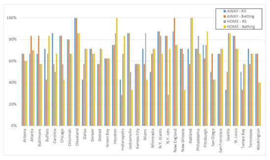
Figure 6. Comparison of accuracy and field for each team.

In Figure 6, the accuracy of the RS regression model and betting are distributed slightly differently for each team. The teams with the largest accuracy gap are Miami, the New York (NY) Jets and New Orleans, in that order. In terms of home and away field factors, Miami and New Orleans have significantly better RS prediction accuracy in the home field than in betting. Conversely, the NY Jets have significantly lower RS prediction accuracy in the home field than in betting. For the three teams in the away field, the gap between the two models is not significant. However, the accuracy of Miami and New Orleans is improved by the RS regression model based on the candlestick characteristics, but the NY Jets remain the furthest behind the betting of the comparison group. Figure 6 also shows that the RS model based on the candlestick chart is prominent when the accuracy of the betting model is less than 50%, including Buffalo’s away, Chicago’s home, Indianapolis’s away, Jacksonville’s home, Miami’s home, New Orleans’s home and Tampa Bay’s away games; this can be improved.

4.4. Discussion and Limitations

The overall performance of the classification-based model was not better than the comparison group, and the best method had just one more correct case. The model seems to give much weight to the input value of LD (t + 1), and its value is close to the actual result. However, the candlestick behaviour can only provide a little adjustment and correction ability according to LD (t + 1). Moreover, the classification-based model reduces the game results to a binary output regardless of the scores of both teams. Regardless of the degree by which the score leads, with a lot of lead or little lead, the result is a win. Given that this study’s hybrid numerical scales and categorical variables are treated as input, the classification-based model is less able to distinguish the score’s degree of leading.

To deal with the problem of forecasting winning/losing, the crucial components are still the numerical scores and the margin of the two teams. Regression models are used to deal with numerical variables, and the predicted values are converted into win/loss. The experimental results of this study also verify that the overall accuracy of the regression-based model is better than the classification-based model and the comparison group. Many studies on win/loss prediction in NFL use a similar approach and deal with numerical variables. Examples have used the win probability [1] of two teams as the output or calculated the rating scores and ranking [3,4,5] of two teams. Finally, the two teams can be compared and the outcome decided.

Moreover, the results of the experiment show that the accuracy of each team is different for the forecasting based on candlesticks and the betting comparison group, which is similar to the phenomenon of technique analysis based on the candlestick chart in the stock market. The candlestick chart of the stock composite index is used to determine the overall behaviour and common pattern. When it is applied to individual stocks for predictions, it produces a different accuracy. Although the behaviour of a sports candlestick is not as rich as that of the stock market, its pattern is not obvious and not easy to interpret. However, it can still be used in the prediction model to reflect the past behaviour of the time series to provide a valuable reference.

Regarding the experimental results of this study, although the best prediction performance is only slightly better compared with the betting market, similar studies have not always presented better performance. As mentioned in the literature, predictive accuracy varies from sport to sport, and an accuracy of near 70% in this study would be promising and acceptable in the case of the NFL.

5. Conclusions and Future Work

This study aimed to predict the outcome of matches in the NFL using machine learning approaches based on candlestick chart characteristics derived from the betting market. This study used the NFL dataset with 13,261 instances composed of the scored points, field and betting market data for 32 seasons. The proposed sports forecasting study based on machine learning contains several features that are different from previous studies, such as following the candlestick technical analysis of the stock market, using data from the betting market rather than considering sports performance and predicting each game from the perspective of two teams individually instead of choosing one out of the home or away teams. To achieve the prediction, we used two approaches, namely, a classification-based model that directly predicted the match outcome and a regression-based model that predicted the winning/losing margin value and then converted it to the match outcome. Consequently, the essence of match outcome prediction could evolve into candlestick pattern recognition in terms of classification or regression. Different machine learning methods for the prediction model, including ensemble learning algorithms, SVMs and neural networks, were evaluated. Considering prediction performance, MB was deemed to be the best solution to the classification approach but is similar to the betting market’s prediction. RS can be regarded as the best solution to the regression approach and yields an accuracy rate of 68.37%, which is slightly better than the betting market’s prediction.

We suggest that the presented approaches based on machine learning and candlestick pattern should be used to investigate the behaviour of each team individually. We also suggest that the prediction of the outcome of the match is evaluated separately by each team or by the offensive and defensive perspective and that the two teams compete against each other to determine the final result. Finally, the information about the candlestick chart for the betting data could be an important tool for increasing the accuracy of sports forecasting in the relevant area.

References

- Lock, D.; Nettleton, D. Using random forests to estimate win probability before each play of an NFL game. J. Quant. Anal. Sports 2014, 10, 197–205. [Google Scholar] [CrossRef]
- Asif, M.; McHale, I.G. In-play forecasting of win probability in One-Day International cricket: A dynamic logistic regression model. Int. J. Forecast. 2016, 32, 34–43. [Google Scholar] [CrossRef]
- Boulier, B.L.; Stekler, H.O. Predicting the outcomes of National Football League games. Int. J. Forecast. 2003, 19, 257–270. [Google Scholar] [CrossRef]
- Hvattum, L.M.; Arntzen, H. Using ELO ratings for match result prediction in association football. Int. J. Forecast. 2010, 26, 460–470. [Google Scholar] [CrossRef]
- Balreira, E.C.; Miceli, B.K.; Tegtmeyer, T. An Oracle method to predict NFL games. J. Quant. Anal. Sports 2014, 10, 183–196. [Google Scholar] [CrossRef][Green Version]
- Haghighat, M.; Rastegari, H.; Nourafza, N. A Review of Data Mining Techniques for Result Prediction in Sports. Adv. Comput. Sci. Int. J. 2013, 2, 7–12. [Google Scholar]
- Albert, J.; Glickman, M.E.; Swartz, T.B.; Koning, R.H. Handbook of Statistical Methods and Analyses in Sports; CRC Press: Boca Raton, FL, USA, 2017. [Google Scholar]
- Leung, C.K.; Joseph, K.W. Sports Data Mining: Predicting Results for the College Football Games. Procedia Comput. Sci. 2014, 35, 710–719. [Google Scholar] [CrossRef]
- Carpita, M.; Ciavolino, E.; Pasca, P. Exploring and modelling team performances of the Kaggle European Soccer database. Stat. Model. 2019, 19, 74–101. [Google Scholar] [CrossRef]
- Stübinger, J.; Mangold, B.; Knoll, J. Machine Learning in Football Betting: Prediction of Match Results Based on Player Characteristics. Appl. Sci. 2020, 10, 46. [Google Scholar] [CrossRef]
- Pratas, J.M.; Volossovitch, A.; Carita, A.I. The effect of performance indicators on the time the first goal is scored in football matches. Int. J. Perform. Anal. Sport 2016, 16, 347–354. [Google Scholar] [CrossRef]
- Bilek, G.; Ulas, E. Predicting match outcome according to the quality of opponent in the English premier league using situational variables and team performance indicators. Int. J. Perform. Anal. Sport 2019, 19, 930–941. [Google Scholar] [CrossRef]
- Metulini, R.; Manisera, M.; Zuccolotto, P. Modelling the dynamic pattern of surface area in basketball and its effects on team performance. J. Quant. Anal. Sports 2018, 14, 117–130. [Google Scholar] [CrossRef]
- Tian, C.; De Silva, V.; Caine, M.; Swanson, S. Use of Machine Learning to Automate the Identification of Basketball Strategies Using Whole Team Player Tracking Data. Appl. Sci. 2019, 10, 24. [Google Scholar] [CrossRef]
- Groll, A.; Schauberger, G.; Tutz, G. Prediction of major international soccer tournaments based on team-specific regularized Poisson regression: An application to the FIFA World Cup 2014. J. Quant. Anal. Sports 2015, 11, 97–115. [Google Scholar] [CrossRef]
- Schauberger, G.; Groll, A. Predicting matches in international football tournaments with random forests. Stat. Model. 2018, 18, 460–482. [Google Scholar] [CrossRef]
- Sarmento, H.; Marcelino, R.; Anguera, M.T.; CampaniÇo, J.; Matos, N.; LeitÃo, J.C. Match analysis in football: A systematic review. J. Sports Sci. 2014, 32, 1831–1843. [Google Scholar] [CrossRef] [PubMed]
- Beal, R.; Norman, T.J.; Ramchurn, S.D. Artificial intelligence for team sports: A survey. Knowl. Eng. Rev. 2019, 34, e28. [Google Scholar] [CrossRef]
- Vračar, P.; Štrumbelj, E.; Kononenko, I. Modeling basketball play-by-play data. Expert Syst. Appl. 2016, 44, 58–66. [Google Scholar] [CrossRef]
- Pai, P.-F.; ChangLiao, L.-H.; Lin, K.-P. Analyzing basketball games by a support vector machines with decision tree model. Neural Comput. Appl. 2017, 28, 4159–4167. [Google Scholar] [CrossRef]
- Horvat, T.; Havaš, L.; Srpak, D. The Impact of Selecting a Validation Method in Machine Learning on Predicting Basketball Game Outcomes. Symmetry 2020, 12, 431. [Google Scholar] [CrossRef]
- Valero, C.S. Predicting Win-Loss outcomes in MLB regular season games—A comparative study using data mining methods. Int. J. Comput. Sci. Sport 2016, 15, 91–112. [Google Scholar] [CrossRef]
- Ul Mustafa, R.; Nawaz, M.S.; Ullah Lali, M.I.; Zia, T.; Mehmood, W. Predicting the Cricket Match Outcome Using Crowd Opinions on Social Networks: A Comparative Study of Machine Learning Methods. Malays. J. Comput. Sci. 2017, 30, 63–76. [Google Scholar] [CrossRef]
- Gu, W.; Foster, K.; Shang, J.; Wei, L. A game-predicting expert system using big data and machine learning. Expert Syst. Appl. 2019, 130, 293–305. [Google Scholar] [CrossRef]
- Baboota, R.; Kaur, H. Predictive analysis and modelling football results using machine learning approach for English Premier League. Int. J. Forecast. 2019, 35, 741–755. [Google Scholar] [CrossRef]
- Knoll, J.; Stübinger, J. Machine-Learning-Based Statistical Arbitrage Football Betting. Künstl. Intell. 2020, 34, 69–80. [Google Scholar] [CrossRef]
- Piasecki, K.; Łyczkowska-Hanćkowiak, A. Representation of Japanese Candlesticks by Oriented Fuzzy Numbers. Econometrics 2019, 8, 1. [Google Scholar] [CrossRef]
- Hu, W.; Si, Y.-W.; Fong, S.; Lau, R.Y.K. A formal approach to candlestick pattern classification in financial time series. Appl. Soft Comput. 2019, 84, 105700. [Google Scholar] [CrossRef]
- Naranjo, R.; Santos, M. A fuzzy decision system for money investment in stock markets based on fuzzy candlesticks pattern recognition. Expert Syst. Appl. 2019, 133, 34–48. [Google Scholar] [CrossRef]
- Fengqian, D.; Chao, L. An Adaptive Financial Trading System Using Deep Reinforcement Learning with Candlestick Decomposing Features. IEEE Access 2020, 8, 63666–63678. [Google Scholar] [CrossRef]
- Li, Y.; Feng, Z.; Feng, L. Using Candlestick Charts to Predict Adolescent Stress Trend on Micro-blog. Procedia Comput. Sci. 2015, 63, 221–228. [Google Scholar] [CrossRef]
- Mallios, W. Sports Metric Forecasting; Xlibris Corporation: Bloomington, IN, USA, 2014; ISBN 978-1-4990-4273-3. [Google Scholar]
- Levitt, S.D. Why are Gambling Markets Organised so Differently from Financial Markets? Econ. J. 2004, 114, 223–246. [Google Scholar] [CrossRef]
- Summers, M. Beating the Book: Are There Patterns in NFL Betting Lines? UNLV Gaming Res. Rev. J. 2008, 12, 43–52. [Google Scholar]
- Williams, L.V. Information Efficiency in Betting Markets: A Survey. Bull. Econ. Res. 1999, 51, 1–39. [Google Scholar] [CrossRef]
- Gray, P.K.; Gray, S.F. Testing Market Efficiency: Evidence from the NFL Sports Betting Market. J. Finance 1997, 52, 1725–1737. [Google Scholar] [CrossRef]
- Mallios, W.S. Forecasting in Financial and Sports Gambling Markets: Adaptive Drift Modeling; John Wiley & Sons: Hoboken, NJ, USA, 2011; ISBN 978-1-118-09953-7. [Google Scholar]
- Štrumbelj, E. On determining probability forecasts from betting odds. Int. J. Forecast. 2014, 30, 934–943. [Google Scholar] [CrossRef]
- Wunderlich, F.; Memmert, D. Analysis of the predictive qualities of betting odds and FIFA World Ranking: Evidence from the 2006, 2010 and 2014 Football World Cups. J. Sports Sci. 2016, 34, 2176–2184. [Google Scholar] [CrossRef]
- Wunderlich, F.; Memmert, D. The Betting Odds Rating System: Using soccer forecasts to forecast soccer. PLoS ONE 2018, 13, e0198668. [Google Scholar] [CrossRef]
- Song, C.; Boulier, B.L.; Stekler, H.O. The comparative accuracy of judgmental and model forecasts of American football games. Int. J. Forecast. 2007, 23, 405–413. [Google Scholar] [CrossRef]
- David, J.A.; Pasteur, R.D.; Ahmad, M.S.; Janning, M.C. NFL Prediction using Committees of Artificial Neural Networks. J. Quant. Anal. Sports 2011, 7, 9. [Google Scholar] [CrossRef]
- Baker, R.D.; McHale, I.G. Forecasting exact scores in National Football League games. Int. J. Forecast. 2013, 29, 122–130. [Google Scholar] [CrossRef]
- Pelechrinis, K.; Papalexakis, E. The Anatomy of American Football: Evidence from 7 Years of NFL Game Data. PLoS ONE 2016, 11, e0168716. [Google Scholar] [CrossRef]
- Schumaker, R.P.; Labedz, C.S.; Jarmoszko, A.T.; Brown, L.L. Prediction from regional angst—A study of NFL sentiment in Twitter using technical stock market charting. Decis. Support Syst. 2017, 98, 80–88. [Google Scholar] [CrossRef]
- Naranjo, R.; Arroyo, J.; Santos, M. Fuzzy modeling of stock trading with fuzzy candlesticks. Expert Syst. Appl. 2018, 93, 15–27. [Google Scholar] [CrossRef]
- Vergin, R.C.; Sosik, J.J. No place like home: An examination of the home field advantage in gambling strategies in NFL football. J. Econ. Bus. 1999, 51, 21–31. [Google Scholar] [CrossRef]
- Goumas, C. Modelling home advantage in sport: A new approach. Int. J. Perform. Anal. Sport 2013, 13, 428–439. [Google Scholar] [CrossRef]
- Lago-Peñas, C.; Gómez-Ruano, M.; Megías-Navarro, D.; Pollard, R. Home advantage in football: Examining the effect of scoring first on match outcome in the five major European leagues. Int. J. Perform. Anal. Sport 2016, 16, 411–421. [Google Scholar] [CrossRef]
- Witten, I.H.; Frank, E.; Hall, M.A.; Pal, C.J. Data Mining: Practical Machine Learning Tools and Techniques; Morgan Kaufmann: Burlington, MA, USA, 2016; ISBN 978-0-12-804357-8. [Google Scholar]
- Breiman, L. Random Forests. Mach. Learn. 2001, 45, 5–32. [Google Scholar] [CrossRef]
- Ho, T.K. The random subspace method for constructing decision forests. IEEE Trans. Pattern Anal. Mach. Intell. 1998, 20, 832–844. [Google Scholar] [CrossRef]
- Webb, G.I. MultiBoosting: A Technique for Combining Boosting and Wagging. Mach. Learn. 2000, 40, 159–196. [Google Scholar] [CrossRef]
- Wang, Y.; Witten, I.H. Induction of Model Trees for Predicting Continuous Classes; Working Paper Series; Department of Computer Science University of Waikato: Hamilton, New Zealand, 1996. [Google Scholar]
- Keerthi, S.S.; Shevade, S.K.; Bhattacharyya, C.; Murthy, K.R.K. Improvements to Platt’s SMO Algorithm for SVM Classifier Design. Neural Comput. 2001, 13, 637–649. [Google Scholar] [CrossRef]
- Shevade, S.K.; Keerthi, S.S.; Bhattacharyya, C.; Murthy, K.R.K. Improvements to the SMO algorithm for SVM regression. IEEE Trans. Neural Netw. 2000, 11, 1188–1193. [Google Scholar] [CrossRef] [PubMed]
- Song, C.; Boulier, B.L.; Stekler, H.O. Measuring consensus in binary forecasts: NFL game predictions. Int. J. Forecast. 2009, 25, 182–191. [Google Scholar] [CrossRef][Green Version]
- Kim, K. Financial time series forecasting using support vector machines. Neurocomputing 2003, 55, 307–319. [Google Scholar] [CrossRef]
© 2020 by the author. Licensee MDPI, Basel, Switzerland. This article is an open access article distributed under the terms and conditions of the Creative Commons Attribution (CC BY) license (http://creativecommons.org/licenses/by/4.0/).