Appraisal of the Spatial Resolution of 2D Electrical Resistivity Tomography for Geotechnical Investigation

Abstract

In the past decade, the 2D electrical resistivity tomography (ERT) has been extensively used in the investigation and monitoring of geotechnical engineering and environment engineering, but there are many uncertainties hidden behind its vivid color earth-resistivity profiles. In order to use the 2D ERT in the scale of geotechnical engineering effectively, the accuracy and spatial resolution capability of measurements must be enhanced, or at least these uncertainties should be mastered to avoid overreading the measurement results. There were seven common geological models built in this study to discuss the variance in spatial analysis capability of 2D electrical resistivity profiles under different geologic conditions. The findings show that the resolution capability of 2D electrical resistivity profiles was influenced by depth, and in different strata, it may be influenced by the resistivity ratio, layer depth, covering depth, interlayer thickness, tilt angle, medium size, and noise intensity. Generally speaking, the relatively low resistance stratum had better resolution capability; if the relatively high resistance stratum was located under the relatively low resistance stratum, its resolution capability declined. In different strata, the resolution capability may be degraded under the effect of different factors. In addition, any noise in the course of measurement resulted in a random jump of the electrical resistivity profile, which worsened as the noise increased. These circumstances should be paid special attention to avoid misrecognition of electrical resistivity profile images.

1. Introduction

In recent years, urban disasters have happened constantly. People’s lives and properties have been increasingly severely threatened. If the geological conditions of the base could provide accurate and detailed information from the prevention perspective of urban disasters, disaster prevention would achieve better results. The incidence of disasters should decline spontaneously.

The investigation of geotechnics aims at the geological conditions of the site. The accurate and detailed information of stratum distribution and material parameters are much required for reference in planning analysis, design, and construction. The more accurate and detailed the geotechnical investigation is, the more suitable countermeasures and construction methods could be proposed in the planning and design stages. It could let the construction period be shortened and expenditures saved. The main traditional method of geotechnical investigation is drilling. However, drilling is expensive and only obtains the information about that point. In addition, the drilling of large sites sometimes fails to meet the planning needs of planners. So, geophysical detection is often used as an assistance method [1,2].

In the past, geophysical exploration was used in geotechnical investigation mostly for seismic detection (refraction, reflection, and surface wave techniques). The elastic wave velocity of strata is closely bound up with the material engineering characteristics [1,2,3], but the seismic detection is likely to be influenced by ambient vibration noise. Moreover, the refraction seismic detection cannot positively detect the low-velocity layer under the high-velocity layer, and the shallow layer (less than 50 m) reflection seismic detection is difficult to be implemented. The surface wave seismic detection consists of mainly 1D and 2D probing techniques; the 3D detection method is still in the preliminary research stage. Ground penetrating radar is a kind of electromagnetic method. The ground penetrating radar is similar to reflection seismic detection, detecting the distribution of the bed boundary, and the localization of depth and the depth of investigation are limited. If a bistatic antenna is used, it can increase the detection depth capability [4,5,6,7]. Electrical resistivity tomography is a kind of electrical method; the present electrical resistivity tomography technique has been able to explore 2D, even 3D earth-resistivity distributions, and the depth of investigation can be adjusted flexibly by the length of the measuring line, and the earth-resistivity is highly correlated with the geomaterial and groundwater characteristics, so it has gradually become one of the main geophysical methods for geotechnical investigation. This study discusses the spatial resolution of 2D ERT in geotechnical investigation.

In the past decade, 2D ERT exploration has been extensively used in geotechnical engineering and environment engineering investigations and monitoring, such as geologic surveys [8,9,10], fault surveys [11,12,13,14,15,16,17], slipping plane surveys and monitoring [18,19,20,21,22,23], groundwater investigations and pollution monitoring [24,25], seawater intrusion investigations [26,27,28,29], dam leakage investigations and monitoring [30,31,32,33], landfill leakage investigations and monitoring [34,35,36,37,38], and archaeological surveys [39,40]. The 3D DC resistance method has been used by scholars [41,42,43], but it is difficult to be implemented, and the site is often limited to the measurement space, so the 2D DC resistance method is still the main method in engineering.

2D ERT has been extensively used in geotechnical engineering investigations, but there are many uncertainties hidden behind the vivid color earth-resistivity profiles. In order to use the 2D ERT in the scale of geotechnical engineering effectively, the accuracy and spatial resolution capability of measurements must be enhanced, or at least these uncertainties should be mastered to avoid overreading the measurement results. This study discusses the variance in 2D electrical resistivity profiles and potential measurement problems; different geologic models were built to discuss the variance in spatial resolution capability of 2D electrical resistivity profiles under different geologic conditions. In addition, the 2D electrical resistivity measurement is often influenced by the boundary effect and 3D effect, so the 2D electrical resistivity profile may be distorted [44]. This study built a numerical model to discuss the results of the two effects.

Therefore, the purpose of this study was to discuss the possible effect of stratigraphic fluctuations on a 2D electrical resistivity profile by numerical simulation and case analysis, and to propose suggestions on interpretation so as to enhance the accuracy of result data interpretation to avoid misrecognition and excessive interpretation.

2. Principle of 2D ERT

The ERT uses two current electrodes (C1, C2) and two potential electrodes (P1, P2) for measurement, as shown in Figure 1. In Figure 1a, the low frequency AC is conducted from the current electrodes to the stratum, in different geometric positions; the potential difference and current are measured by using potential electrodes and current electrodes, and then the apparent resistivity is theoretically calculated by electrostatics, expressed as Equation (1) [45]:

$$\begin{array}{l}\rho =K\frac{\Delta V}{I}; \Delta V=V_{P1}-V_{P2}\\ K=\frac{2\pi }{\left(\frac{1}{R_1}-\frac{1}{R_2}-\frac{1}{R_3}+\frac{1}{R_4}\right)}\end{array}$$

(1)

where K is the geometric parameter of the electrode array, ΔV is the potential difference measured by potential electrodes, I is the input current strength, R1 is equal to the distance between C1 and P1, R2 is equal to the distance between C2 and P1, R3 is equal to the distance between C1 and P2, and R4 is equal to the distance between C2 and P2. The apparent resistivity represents the resistivity measured by the electrical resistivity method when the medium is homogeneous [45]. During the measurement in real strata, the resistivity of the subject may be heterogeneous, and the resistivity measured by changing the electrode spacing and location thus change. Therefore, if tens of electrodes are laid equidistantly on the earth’s surface at first, the pseudo-section can be obtained by continuously changing the spacing and horizontal movement of the aforesaid paired current electrodes and potential electrodes. Figure 1b shows the pseudo-section measured by using a Wenner arrangement of electrodes [46]. Finally, the resistivity profile representing strata can be obtained by inverse computation analysis. The inverse analysis generally uses the optimized method. The inverse calculation software first estimates the initial value of the inverse calculation model by measuring the pseudo-section of the resistivity. After the initial model of inverse calculation is given, the difference between the response values and the measured data of the model is minimized by multiple operations. Thus, the result of this inverse calculation is the resistivity profile of real strata.

3. Research Method

3.1. Analysis of Problems in ERT

The measurement results of ERT in geotechnical engineering investigations are often compared with drilling well data. It could be preliminarily determined whether the image change of the geo-resistance profile coincides with the stratigraphic change of the drilling well. However, the change of resistivity would be affected by various factors including soil water content, geological structure, groundwater level, and surrounding noise. The results of the measurement would affect the sensitivity and spatial analysis of the results of the ERT measurement. Therefore, the measurement still has the problem of spatial analysis ability, especially for the identification of the layer position and the interlayer thickness, the change of the inclined stratum, the detection of the underground target, and the factors such as the limitation of the boundary conditions around the survey line and the 3D effect. The interactive influence of various influencing factors would influence the accuracy of the result’s interpretation.

The interpretation of ERT measurement results is often a significant challenge for engineers. This study analyzed and explained the related problems commonly encountered in the interpretation of resistivity profile as follows:

3.1.1. Problems in the Spatial Resolution Capability of the Resistivity Profile

Electrical resistivity images have been extensively used in geotechnical engineering investigations, but the interpretation of images has not yet been discussed specifically. Due to stratal configuration changes and environmental changes, the obtained resistivity profiles have different levels of representativeness, resulting in difficult interpretations. How to enhance the interpretative capability by discussing resolution capability?

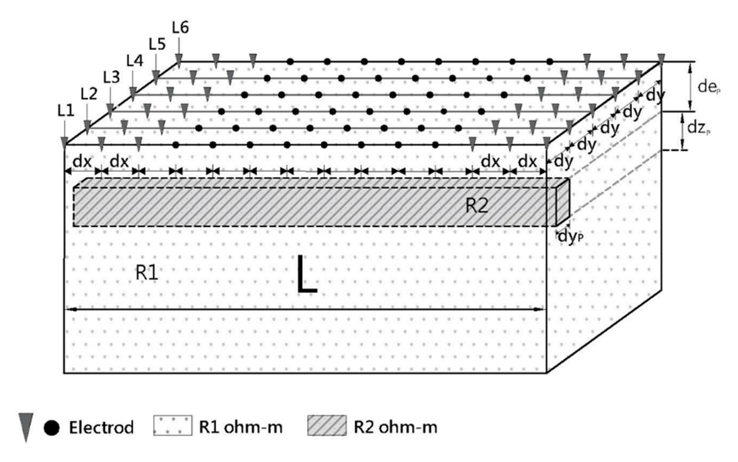
3.1.2. Influence of the Boundary Effect

In terms of the boundary effect, the 2D ERT measurement is performed on a straight line of finite length, but if there are topographical changes on two lateral boundaries of the measuring line, e.g., ponds, valleys, or substructures like concrete structures or metal pipelines, the resistivity may be mapped onto the 2D electrical resistivity profile, inducing detection errors, and influencing the measurement result and interpretation accuracy.

3.1.3. Influence of the 3D Effect

The linear 2D electrical resistivity tomography assumes that the formation resistivity property is homogeneous in the direction normal to the measuring line; when the stratum is not homogeneous in the direction normal to the measuring line, as the current flows in a 3D direction, there may be errors in the 2D electrical prospecting result. The distortion, which may be induced by this assumption, is often neglected in the interpretation of measurement results. The 3D effect is the detection error induced by mapping the resistivity of the geologic configuration outside the 2D electrical resistivity profile (normal to the measuring line) onto the 2D electrical resistivity profile. In the course of inverse computation, the result of convergence based on certain assumptions (e.g., 2D assumptions) may mismatch onsite 3D conditions. In addition, the numerical model assumed in inverse computation is assumed to execute operations on the mesh of finite space and volume, mismatching the field of infinite space. Therefore, there are 3D and boundary effects on the 2D electrical resistivity profile.

3.2. Build Geological Models

In order to know the effect of stratigraphic fluctuation on the electrical resistivity profile, this study planned several geological models for common strata to simulate the conditions of onsite strata, so as to perform numerical simulation, and to discuss the resolution capability of different models. There are seven kinds of geological models, such as the single horizontal layer stratum, horizontal interlayer stratum, single vertical layer stratum, vertical interlayer stratum, composite stratum, tilted layer stratum, and debris mixed stratum. This study used the analytical software Res2dmod [47] developed by Geotomo for numerical simulation and used Res2dinv software [48] for inverse computation analysis. The direct computation simulation used the finite element method to calculate the apparent resistivity value of the built stratum model. The inverse computation analysis method used the optimal least squares method (L2 norm) to calculate the final electrical resistivity profile chart of the model because the L2 norm is more suitable for progressive strata.

After several geological models were built, the differences in the electrical resistivity profile chart were discussed according to parameter variation; correlated influencing parameters were taken according to the characteristics of geological models from the resistivity ratio, layer depth, interlayer thickness, tilt angle, medium size, and noise intensity for discussion. In this study, 96 electrode rods were set; the spacing distance was d = 2 m, and the measurement line length was L = 190 m. Because Wenner has higher sensitivity and a stronger signal strength for vertical resolution analysis, it is most widely used in on-situ measurements. Therefore, Wenner was used as the simulation application method in this study.

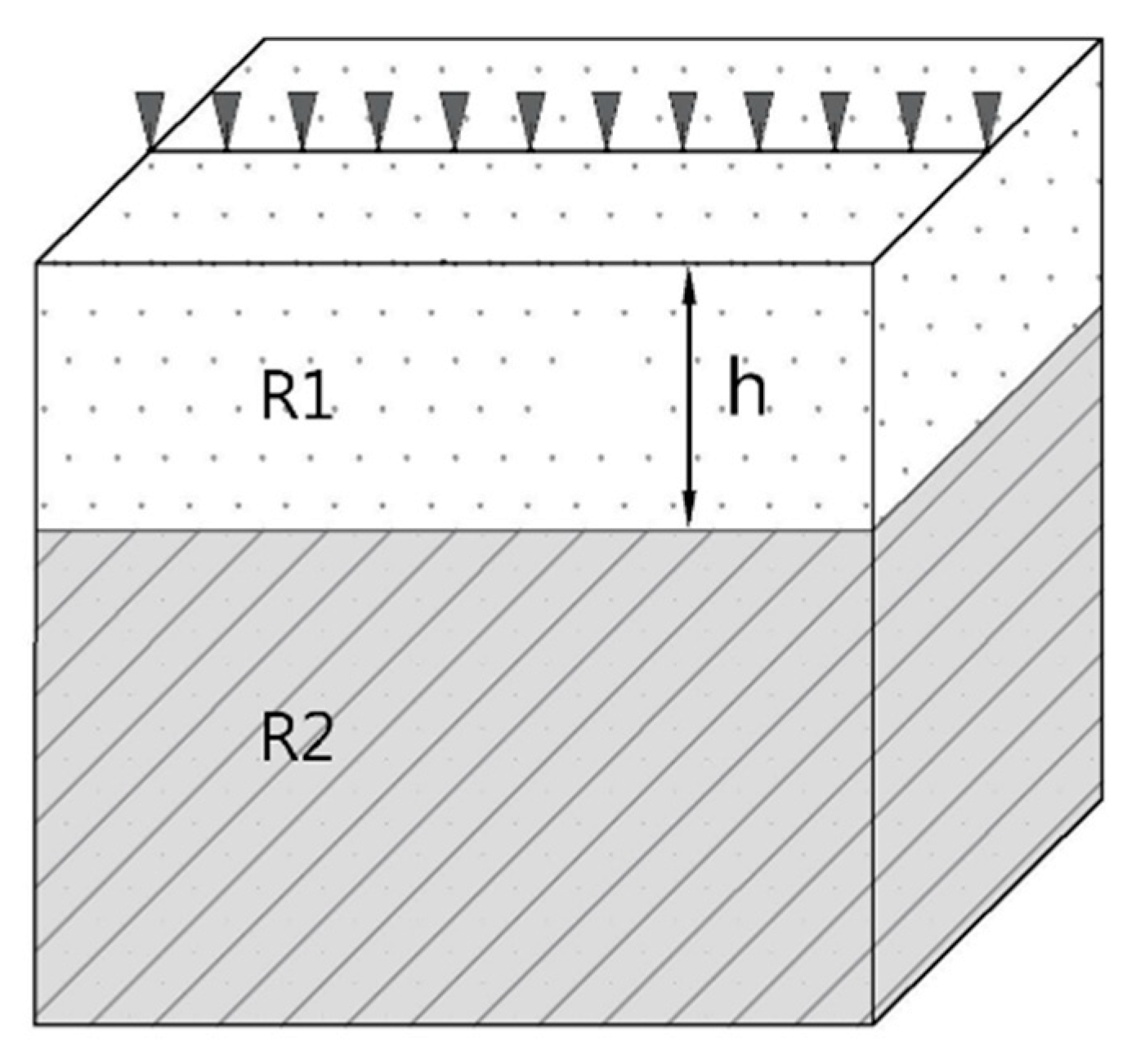
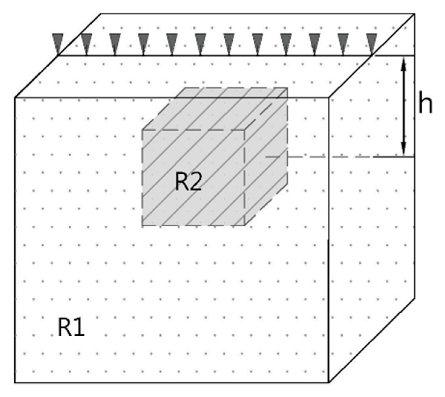
3.2.1. Single Horizontal Layer Stratum Model

The horizontal layer is the most familiar stratum. Figure 2 is the schematic diagram of the single horizontal layer stratum model. This study discusses the effect of different resistivities, layer depths, and noise intensities. The upper resistivity is R1, and the lower resistivity is R2. Different resistivities were set up for comparison. There were eight groups of resistivity variation, which were (R1, R2) = (R1 = 50, R2 = 500, 200, 150, 75) and (R1 = 500, 200, 150, 75, R2 = 50). The layer depth is h; the depths were set as 10 m and 20 m. The noise interference generated by the ambient environment was set up by Gaussian noise. The Gaussian noises were set as 0%, 2%, 4%, 6%, and 8%.

Table 1. Parameter table of the single horizontal layer stratum model.

Single Horizontal Layer Stratum Model
Impact Factors	n		R1	R2	h	N
Resistivity ratio (n = R1/R2)	n < 1	0.1	50	500	10	0
		0.25		200
		0.33		150
		0.66		75
	n > 1	10	500	50	10	0
		4	200
		3	150
		1.5	75
Layer depth (h)	n < 1	0.25	50	200	10	0
					20
	n > 1	4	200	50	10	0
					20
Noise intensity (N)	n < 1	0.25	50	200	10	0–8%
	n > 1	4	200	50	10	0–8%

shows the parameters of the single horizontal layer stratum model.

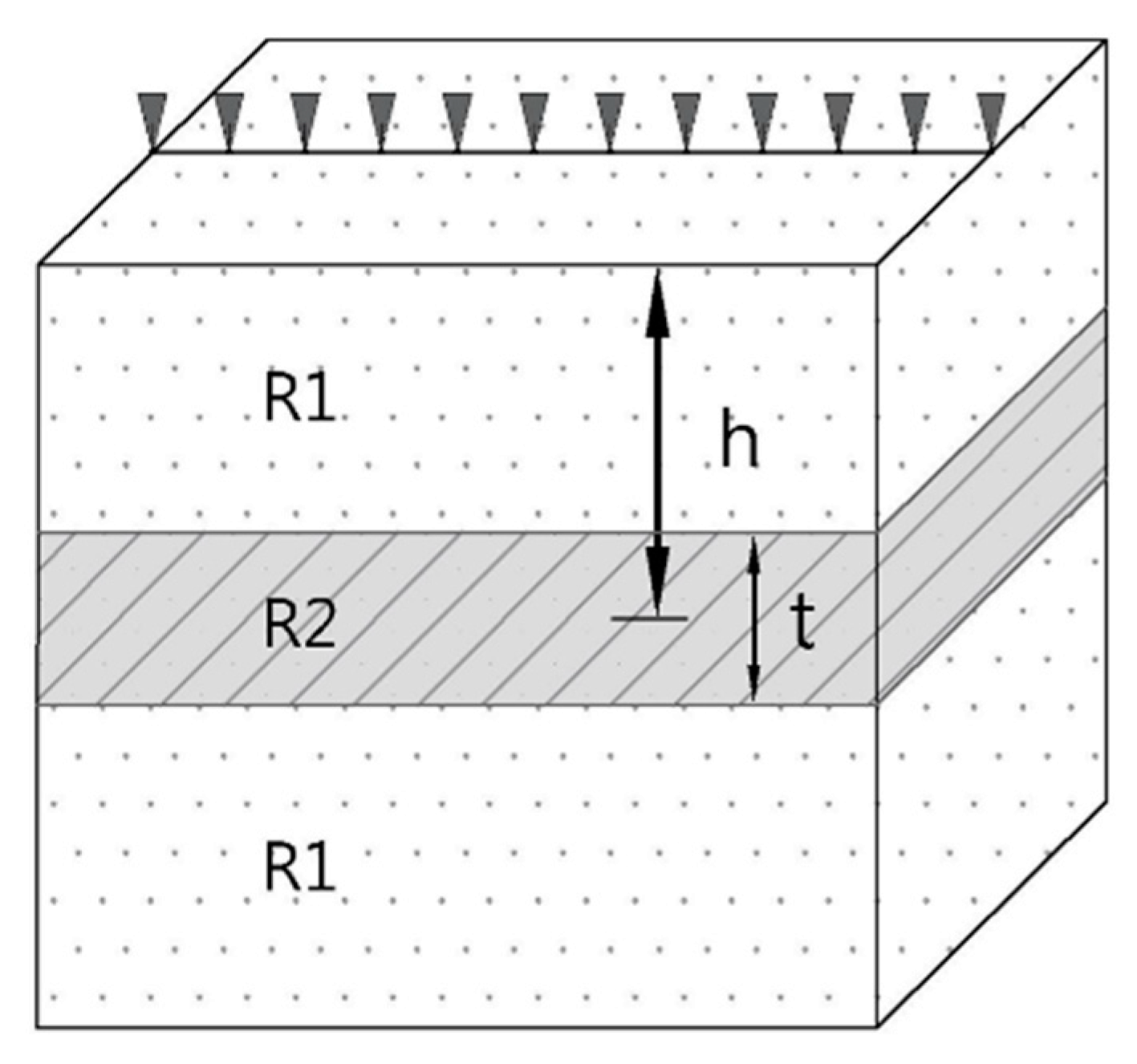
3.2.2. Horizontal Interlayer Stratum Model

The horizontal interlayer stratum is usually an inhomogeneous stratum or a stratum with only one layer. Figure 3 is the schematic diagram of the horizontal interlayer stratum model. The upper and lower resistivity of the layer is R1, and the interlayer is R2; the effect of different resistivities, interlayer center depths, interlayer thicknesses, and noise intensities are discussed. There were eight groups of resistivity variation, which were (R1, R2) = (R1 = 50, R2 = 500, 200, 150, 75) and (R1 = 500, 200, 150, 75, R2 = 50). The interlayer center depth h was set as 10 m and 16 m for discussion. The interlayer thickness t was set as 4 m and 8 m, and the noise interference generated by the ambient environment was set up by Gaussian noise: the Gaussian noise was set as 0%, 2%, 4%, 6%, and 8%, respectively.

Table 2. Parameter table of the horizontal interlayer stratum model.

Horizontal Interlayer Stratum Model
Impact Factors	n		R1	R2	h	t	N
Resistivity ratio (n = R1/R2)	n < 1	0.1	50	500	10	8	0
		0.25		200
		0.33		150
		0.66		75
	n > 1	10	500	50	10	8	0
		4	200
		3	150
		1.5	75
Interlayer center depth (h)	n < 1	0.25	50	200	10	8	0
					20
	n > 1	4	200	50	10
					20
Interlayer thickness (t)	n < 1	0.25	50	200	10	8	0
						4
	n > 1	4	200	50		8
						4
Noise intensity (N)	n < 1	0.25	50	200	10	8	0–8%
	n > 1	4	200	50	10	8	0–8%

shows the parameters of the horizontal interlayer stratum model.

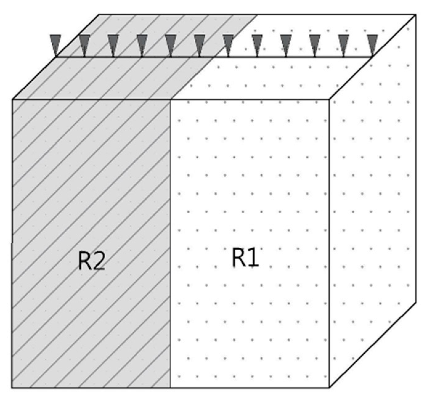
3.2.3. Single Vertical Layer Stratum Model

Besides the horizontal layer stratum, there is an approximately vertical layer stratum, so this study built a single vertical layer stratum model for analysis, as shown in Figure 4. The right and left resistivities of the layer were R1 and R2 for the results of different resistivities and different noise intensities. There were four groups of resistivity variation, which were (R1, R2) = (R1 = 50, R2 = 500, 200, 150, 75). The noise interference generated by the ambient environment was set up by Gaussian noise. The Gaussian noise was set as 0%, 2%, 4%, 6%, and 8%, respectively.

Table 3. Parameter table of the single vertical interlayer stratum model.

Single Vertical Layer Stratum Model
Impact Factors	n	R1	R2	Noise
Resistivity ratio (n = R1/R2)	0.1	50	500	0
	0.25		200
	0.33		150
	0.66		75
Noise intensity (N)	0.25	50	200	0–8%

shows the parameters of the single vertical interlayer stratum mode.

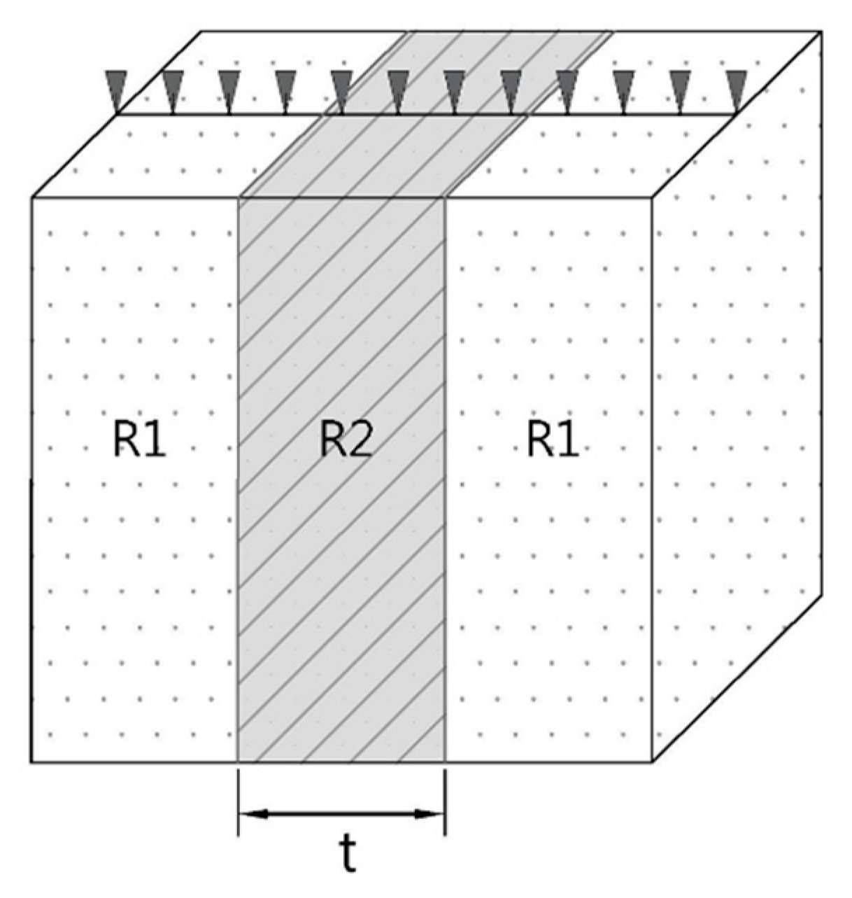
3.2.4. Vertical Interlayer Stratum Model

A vertical interlayer stratum model was built for analysis, as shown in Figure 5. The resistivity of the right and left levels of stratum is R1, and the resistivity of the interlayer is R2; the results of different resistivities, interlayer thicknesses, and noise intensities are discussed. There were eight groups of resistivity variation, which were (R1, R2) = (R1 = 50, R2 = 500, 200, 150, 75) and (R1 = 500, 200, 150, 75, R2 = 50). The interlayer thickness t was set as 10 m and 20 m. The noise interference generated by the ambient environment was set up by Gaussian noise. The Gaussian noise was set as 0%, 2%, 4%, 6%, and 8%, respectively.

Table 4. Parameter table of the vertical interlayer stratum model.

Vertical Interlayer Stratum Model
Impact Factors	n		R1	R2	t	Noise
Resistivity ratio (n = R1/R2)	n < 1	0.1	50	500	10	0
		0.25		200
		0.33		150
		0.66		75
	n > 1	10	500	50	10	0
		4	200
		3	150
		1.5	75
Interlayer thickness (t)	n < 1	0.25	50	200	10	0
					20
	n > 1	4	200	50	10
					20
Noise intensity (N)	n < 1	0.25	50	200	8	0–8%
	n > 1	4	200	50	8	0–8%

shows the parameters of the vertical interlayer stratum model.

3.2.5. Composite Stratum Model

There are other materials in the strata, such as pipelines, water ditches, or underground pillboxes. Therefore, this study built a composite stratum model for analysis, as shown in Figure 6. A square homogeneous material was created in the stratum. The resistivity of this material is R2. The resistivity of the background soil layer is R1. The results of different resistivities, different depths, and different noise intensities are discussed. There were eight groups of resistivity variation, which were (R1, R2) = (R1 = 50, R2 = 500, 200, 150, 75) and (R1 = 500, 200, 150, 75, R2 = 50). The material center depth h was set as 10 m and 20 m. The noise interference generated by the ambient environment was set up by Gaussian noise. The Gaussian noise was set as 0%, 2%, 4%, 6%, and 8%, respectively.

Table 5. Parameter table of the composite stratum model.

Composite Stratum Model
Impact Factors	n		R1	R2	h	Noise
Resistivity ratio (n = R1/R2)	n < 1	0.1	50	500	10	0
		0.25		200
		0.33		150
		0.66		75
	n > 1	10	500	50	10	0
		4	200
		3	150
		1.5	75
Material center depth (h)	n < 1	0.25	50	200	10	0
					20
	n < 1	4	200	50	10
					20
Noise intensity (N)	n < 1	0.25	50	200	10	0–8%
	n > 1	4	200	50	10	0–8%

shows the parameters of the composite stratum model.

3.2.6. Tilted Layer Stratum Model

The tilted layer is a common geological structure of faults. In order to know the electrical resistivity profile resolution capability of tilted layers, this study built a tilted layer stratum model for analysis, as shown in Figure 7. The resistivity of the upper soil layer is R1, and the resistivity of the lower soil layer is R2; different resistivities, different tilt angles, and different noise intensities are discussed. The layer depth of the model was h = 20 m. There were eight groups of resistivity variation, which were (R1, R2) = (R1 = 50, R2 = 500, 200, 150, 75) and (R1 = 500, 200, 150, 75, R2 = 50). The tilt angle α was set as 30° and 60°. The noise interference generated by the ambient environment was set up by Gaussian noise. The Gaussian noise was set as 0%, 2%, 4%, 6%, and 8%, respectively.

Table 6. Parameter table of the tilted layer stratum model.

Tilted Layer Stratum Model
Impact Factors	n		R1	R2	α	Noise
Resistivity ratio (n = R1/R2)	n < 1	0.1	50	500	60	0
		0.25		200
		0.33		150
		0.66		75
	n > 1	10	500	50	60	0
		4	200
		3	150
		1.5	75
Tilt angle (α)	n < 1	0.25	50	200	60	0
					30
	n > 1	4	200	50	60
					30
Noise intensity (N)	n < 1	0.25	50	200	60	0–8%
	n > 1	4	200	50	60	0–8%

shows the parameters of the tilted layer stratum model.

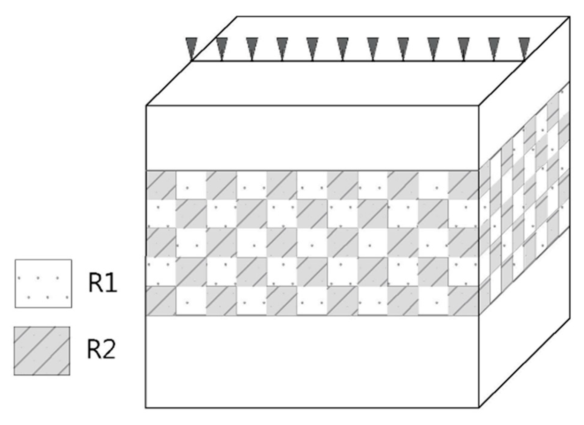
3.2.7. Debris Mixed Stratum Model

The colluvium and debris flow often have debris entrainment, so this study built a debris mixed stratum model for analysis, as shown in Figure 8, so as to enhance the ability to interpret this kind of stratum. As the debris mixed layer entrains a lot of stones, the model was configured with mosaic mesh, so as to simulate the debris mixed stratum. The resistivity of the background soil layer is R1, and the resistivity of the medium in the soil layer is R2. Different resistivities, covering depths, mesh sizes, mesh spacings, and noise intensities are discussed. There were eight groups of resistivity variation, which were (R1, R2) = (R1 = 50, R2 = 500, 200, 150, 75) and (R1 = 500, 200, 150, 75, R2 = 50). The covering depth h was set as 0 m and 10 m. The mesh area was set as 2m × 2m and 4m × 4m. The mesh spacing was set as 2 m and 4 m. The noise interference generated by the ambient environment was set up by Gaussian noise. The Gaussian noise was set as 0%, 2%, 4%, 6%, and 8%, respectively.

Table 7. Parameter table of the debris mixed stratum model.

Debris Mixed Stratum Model
Impact Factors	n		R1	R2	h	A	S	Noise
Resistivity ratio (n = R1/R2)	n < 1	0.1	50	500	0	2 × 2	2	0
		0.25		200
		0.33		150
		0.66		75
	n > 1	10	500	50	0	2 × 2	2	0
		4	200
		3	150
		1.5	75
Covering depths (H)	n < 1	0.25	50	200	0	2 × 2	2	0
					10
	n > 1	4	200	50	0
					10
Mesh sizes (A)	n < 1	0.25	50	200	0	2 × 2	2	0
						4 × 4
	n > 1	4	200	50	0	2 × 2		0
						4 × 4
Mesh spacings (S)	n < 1	0.25	50	200	0	2 × 2	2	0
	n > 1	4	200	50			4
Noise intensity (N)	n < 1	0.25	50	200	0	2 × 2	2	0–8%
	n > 1	4	200	50	0	2 × 2	2	0–8%

shows the parameters of the debris mixed stratum model.

3.3. Discussion About the Boundary Effect

In order to know the boundary effect, which may be induced by stratigraphic fluctuations on both sides of the measuring line, this study built a numerical model of stratigraphic fluctuation at the measuring line boundary; the influence of the boundary effect on 2D electrical resistivity profiles is discussed by numerical simulation according to the changes in the boundary medium. If the boundary had a heterogeneous medium, the model with a boundary effect was compared with the model without boundary effect to discuss the differences. Figure 9 is the schematic diagram of the boundary effect model. This study discusses boundary effect distances. The background resistivity of the soil layer was set as R1 in the model; the boundary medium resistivity was R2; the resistivity ratio was n = R2/R1, (R1, R2) = (1000, 10); the section size of the medium was dyp × dzp, set as 2 m × 2 m; the depth of burying dep was set as 2 m; the electrode spacing dx was set as 2 m; and the measuring line length was L = 50 m. As the dipole–dipole has better resolution capability for lateral variation, the measuring line configuration was dipole–dipole in this study.

Table 8. Parameter table of the boundary effect model.

Boundary Effect Model
Impact Factors	n	R1	R2	dx	dep	dyp	dzp	L
Influence distance	0.01	1000	10	2	2	2	2	50

shows the parameters of the boundary effect model.

3.4. 3D Effect Analysis

When the measuring line measurement violates the assumption of the 2D electrical resistivity method that the formation resistivity property is homogeneous in the direction normal to the measuring line, the 3D effect is generated, influencing the measurement result. As the electrical resistivity measurement is the current field solving in 3D space, this study used the universal finite element analysis software COMSOL 4.2a-AC/DC module to build a 3D direct computation model (COMSOL group, 2011). This study assumed that the strata had pipelines, and the measuring line distance was changed to discuss the interaction. Figure 10 is the schematic diagram of the 3D effect model. The pipeline resistivity was set as R2 in the model, and the soil layer resistivity was R1; if the resistivity ratio was n = R2/R1, (R1, R2) = (1000, 100), the section size of pipeline was dyp × dzp, set as 1.5 m × 2 m, and the depth of burying dep was set as 2 m. There were 5 to 6 measuring lines laid in parallel with the pipeline. The distance dy between measuring lines was set as 3 m, the electrode spacing dx was set as 3 m, and the measuring line length was L = 42m. As the dipole–dipole has better resolution capability for lateral variation, the measuring line configuration was dipole–dipole in this study.

Table 9. Parameter table of the 3D effect model.

3D Effect Model
Impact Factors	n	R1	R2	dx	dep	dyp	dzp	L
Influence distance	1000	100	3	3	2	1.5	2	42

shows the parameters of the 3D effect model.

4. Results and Discussion

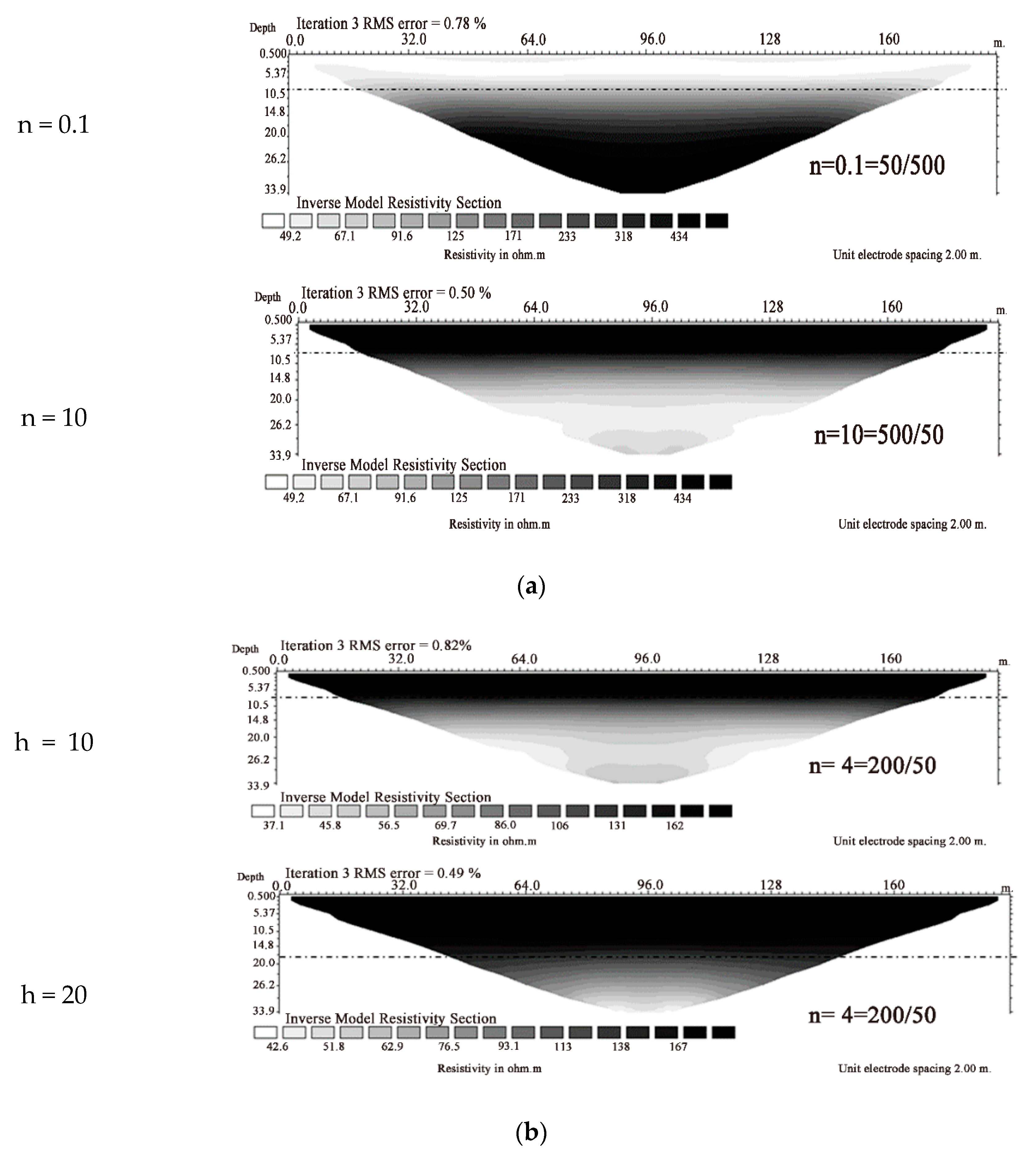
4.1. Single Horizontal Layer Stratum Model

The results of Single Horizontal Layer Stratum as shown in Figure 11. The single horizontal layer stratum usually had better resolution capability when the low resistance was in the upper layer or lower layer because the current flowed in the lower resistivity layer, leading to higher resolution capability. If the high resistance was in the upper layer, the resolution capability was good. However, when the high resistance was in the lower layer, the resolution capability began to decline under the effect of low resistance in the upper layer. Different resistivities of upper and lower layers resulted in gradation zones nearby the layer; the main gradation zone was in the lower layer, and the difference value of the gradation zone increased with the difference between R1 and R2, as shown in Figure 11a. The larger the layer depth was, the lower was the resolution capability, as shown in Figure 11b. There was noise interference in the course of measurement; the resistivity profile had a random jump. The jump worsened as the noise increased, as shown in Figure 11c.

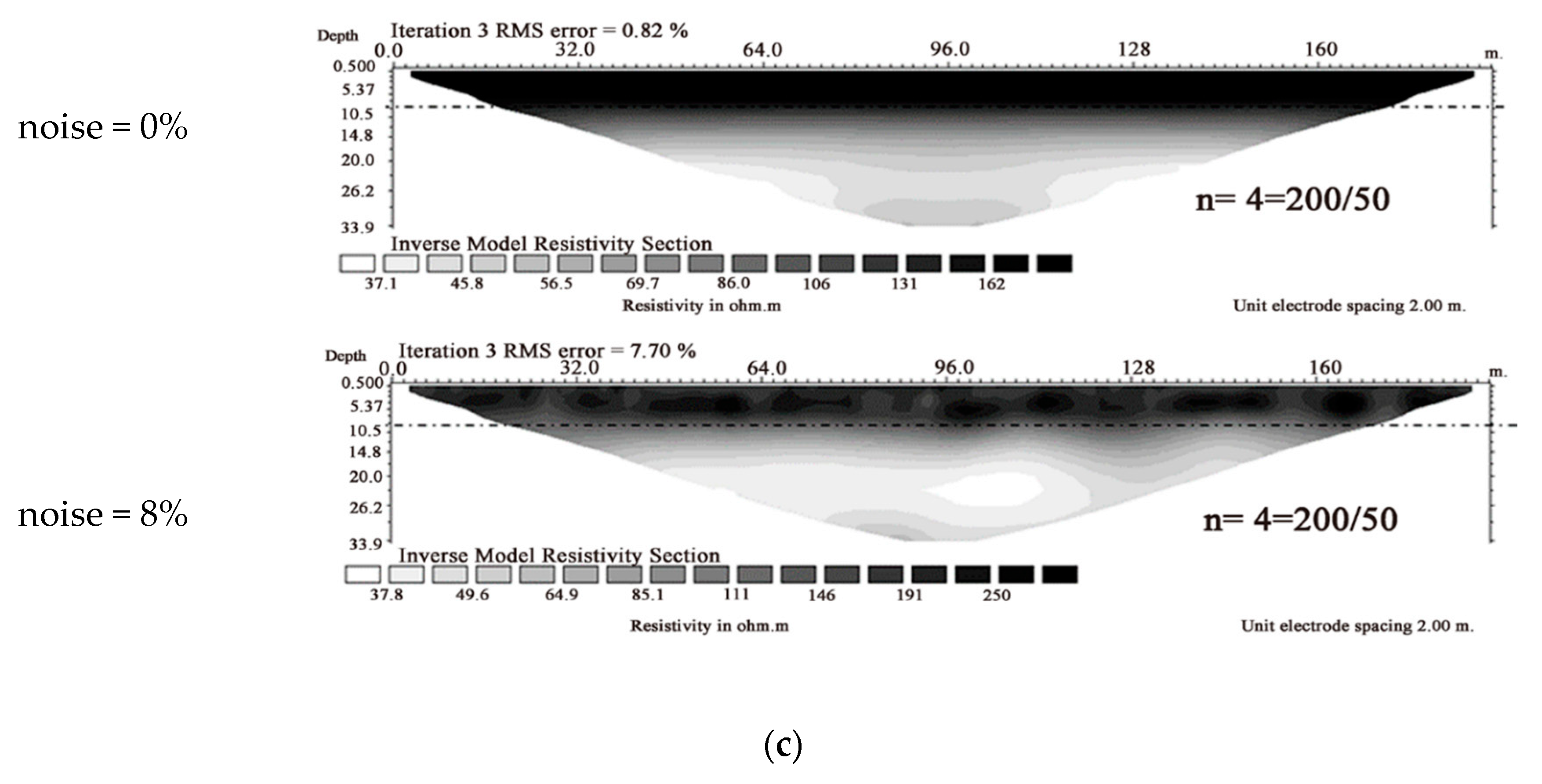
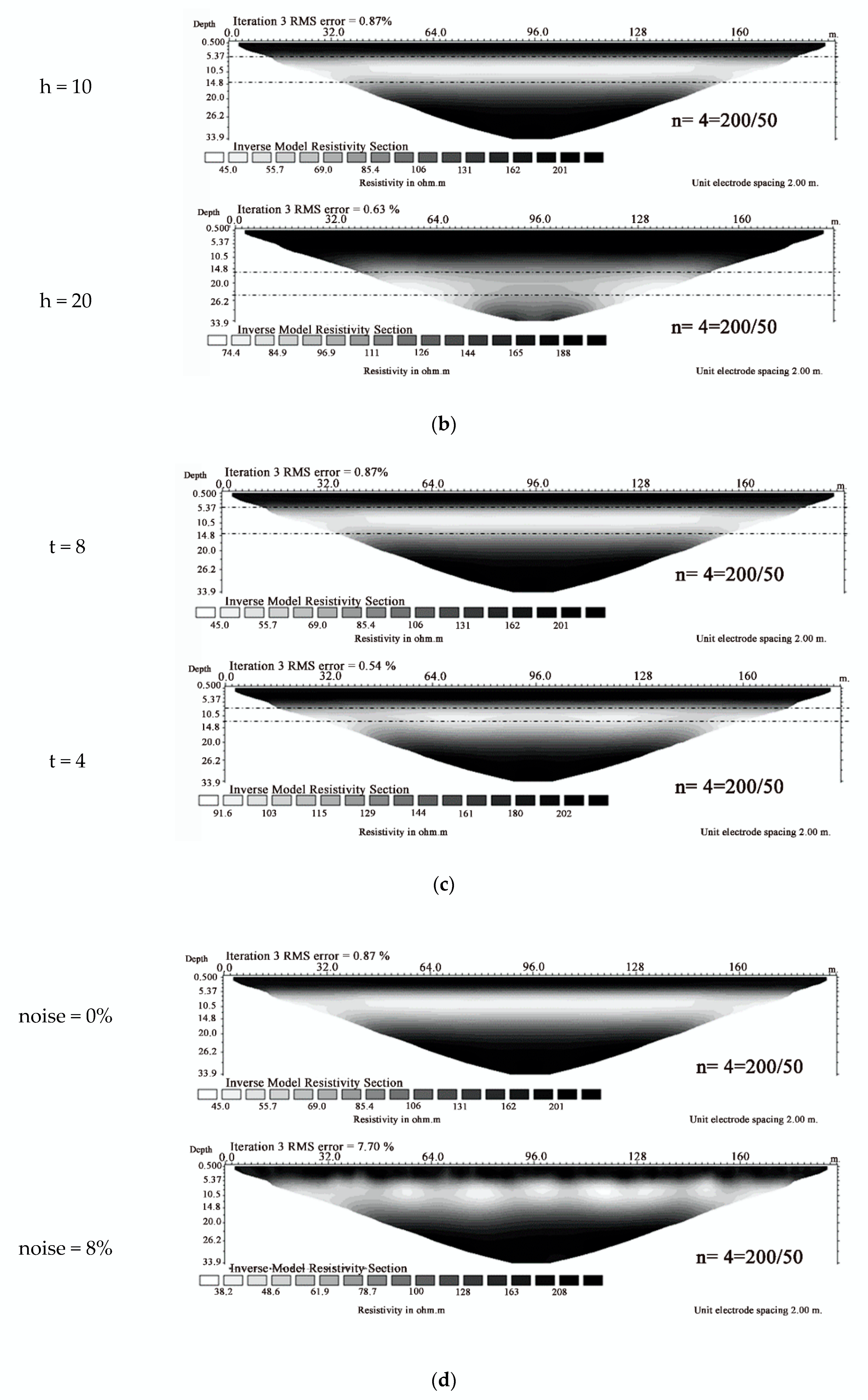
4.2. Horizontal Interlayer Stratum Model

The results of Horizontal Interlayer Stratum as shown in Figure 12. In the horizontal interlayer stratum, when the low resistance region was in the upper and lower layers or interlayer, the resistivity equivalent to the set value could be obtained, but when the high resistance was in the lower layer of the interlayer, the resistivity decreased under the effect of the low resistance interlayer, and it was difficult to interpret the layer. Whatever the n value was, there was a gradation zone nearby the layer. When the R1 was close to the R2 value, the interlayer was replaced by the gradation zone gradually, and the thickness decreased gradually, as shown in Figure 12a. The larger the interlayer center depth was, the worse was the resolution capability, and the identification even failed, as shown in Figure 12b. If the interlayer thickness became half of the original value (4 m), the detected thickness was larger than 4 m, and the resistivity of the interlayer was different from the set value, as shown in Figure 12c. When there was noise interference in the detection process, the resistivity profile had a random jump, the interlayer became nonlaminar, and the jump worsened as the noise increased, as shown in Figure 12d.

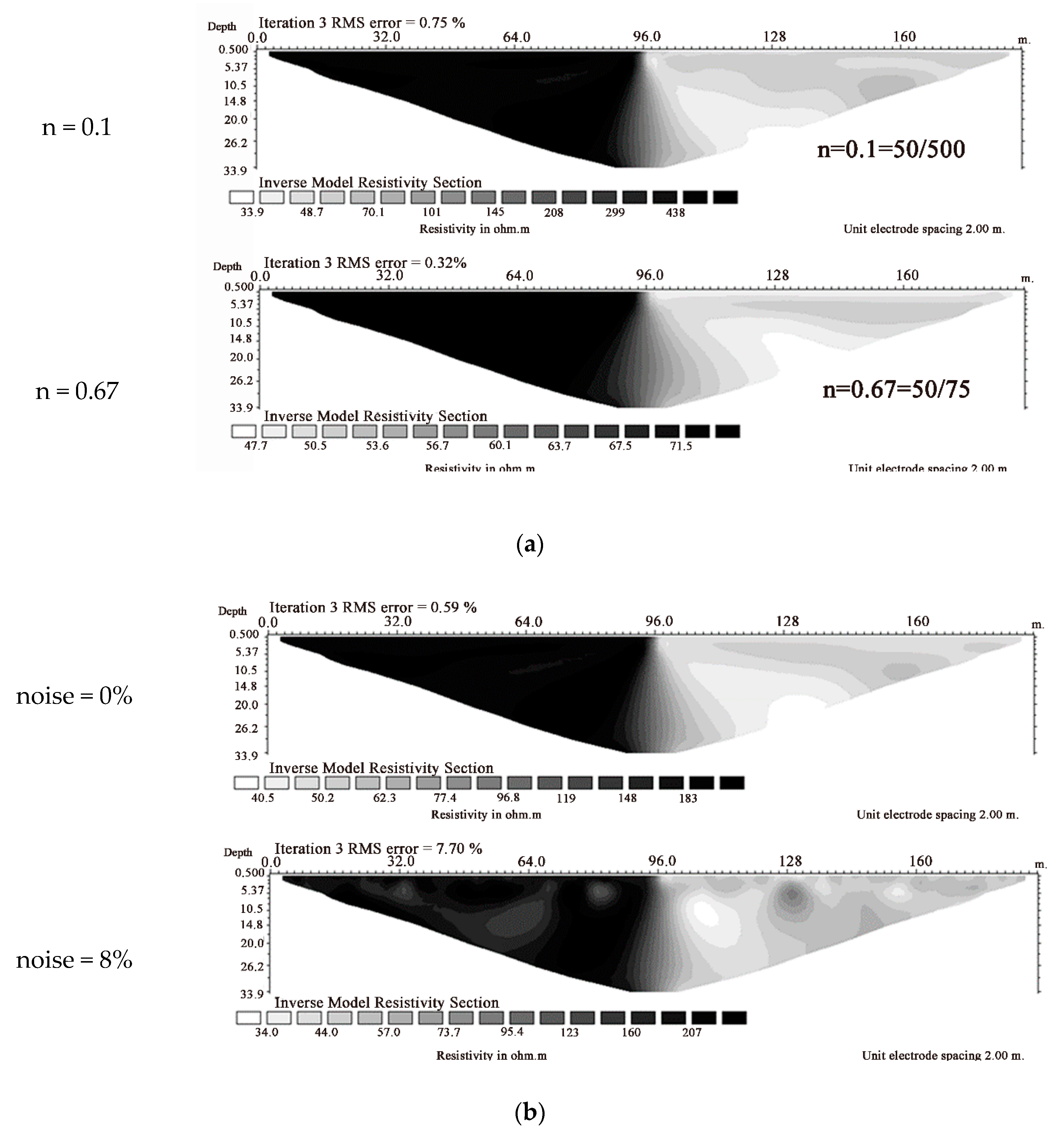
4.3. Single Vertical Layer Stratum Model

The results of Single Vertical Layer Stratum as shown in Figure 13. There was a large gradation zone in the single vertical layer stratum, and it was difficult to clarify the vertical layer; the vertical layer could be identified clearly within 8 M. As the R1 became closer to the R2 value, the gradation zone widened gradually, but the range outside the gradation zone was identical with the set value, as shown in Figure 13a. When there was noise interference in the detection process, the resistivity profile had a random jump. The random jump worsened as the noise increased, and the resistivity of the left and right layers was different from the set value, as shown in Figure 13b.

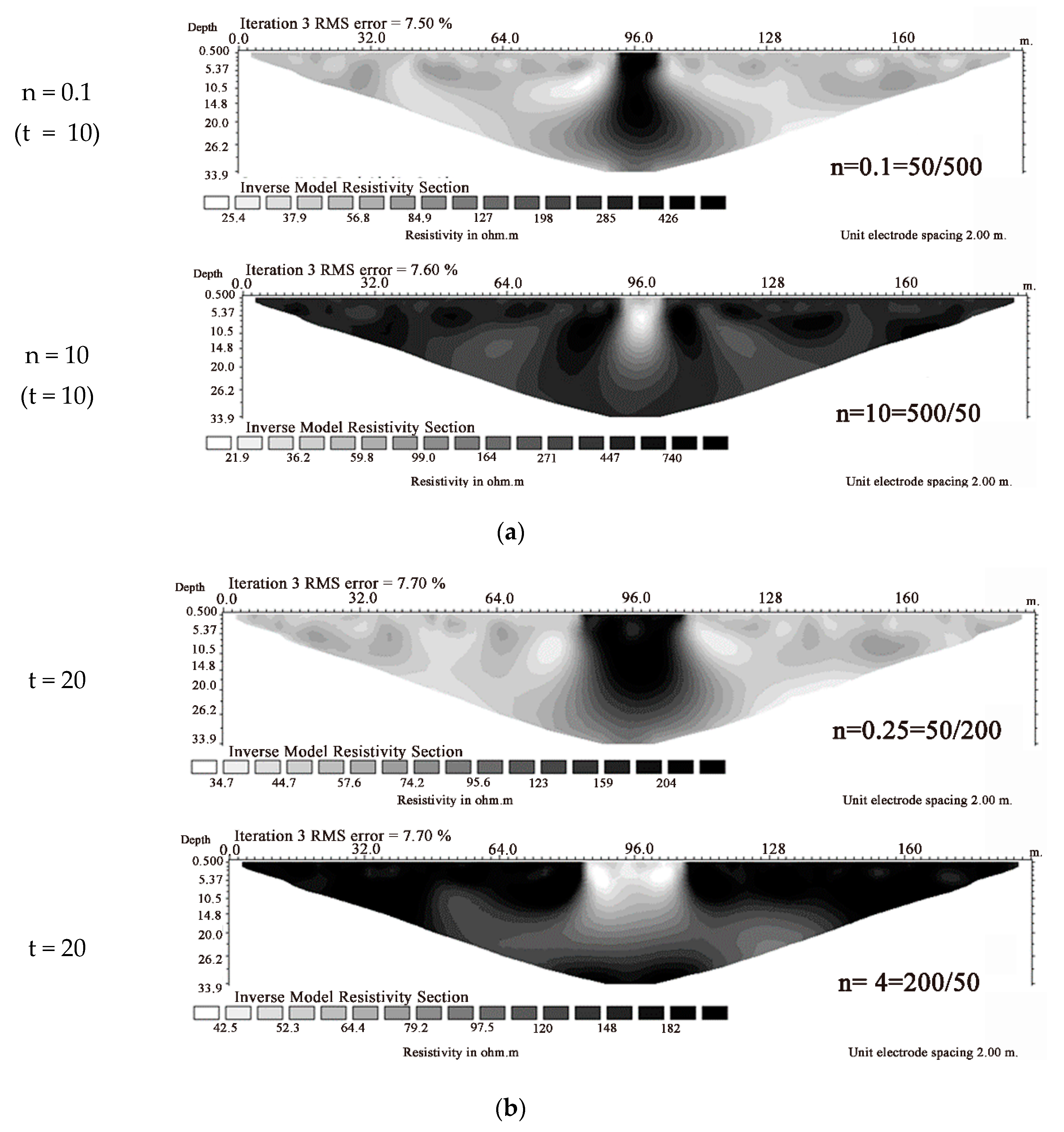
4.4. Vertical Interlayer Stratum Model

The results of Vertical Interlayer Stratum as shown in Figure 14. In the vertical interlayer stratum, there were gradation zones under the interlayer. When the interlayer was a relatively high resistance region, the deeper interlayer could be identified clearly. The closer the R1 was to the R2 value, the lower the identifiable depth of the interlayer, as shown in Figure 14a. When the interlayer was a relatively high resistance region, the identifiable depth increased with interlayer thickness. However, when the interlayer was a relatively low resistance region, the identifiable depth remained constant as the interlayer thickness increased, and the interlayer and the region outside the interlayer had jumping phenomena, as shown in Figure 14b. When there was noise interference in the detection process, the resistivity profile had a random jump; the random jump worsened as the noise increased, but the identifiable depth of the interlayer was free from the effect of noise, as shown in Figure 14c.

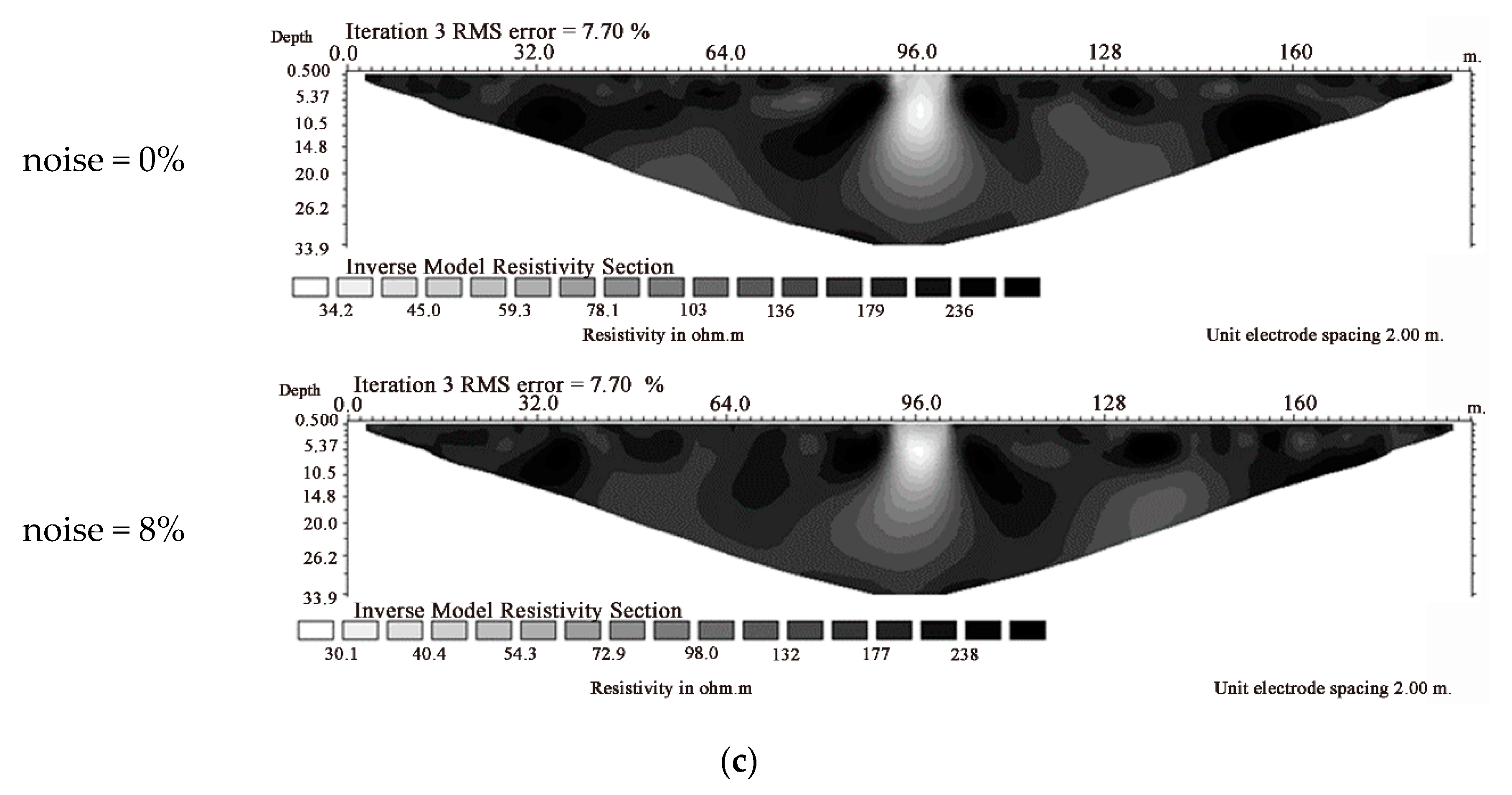
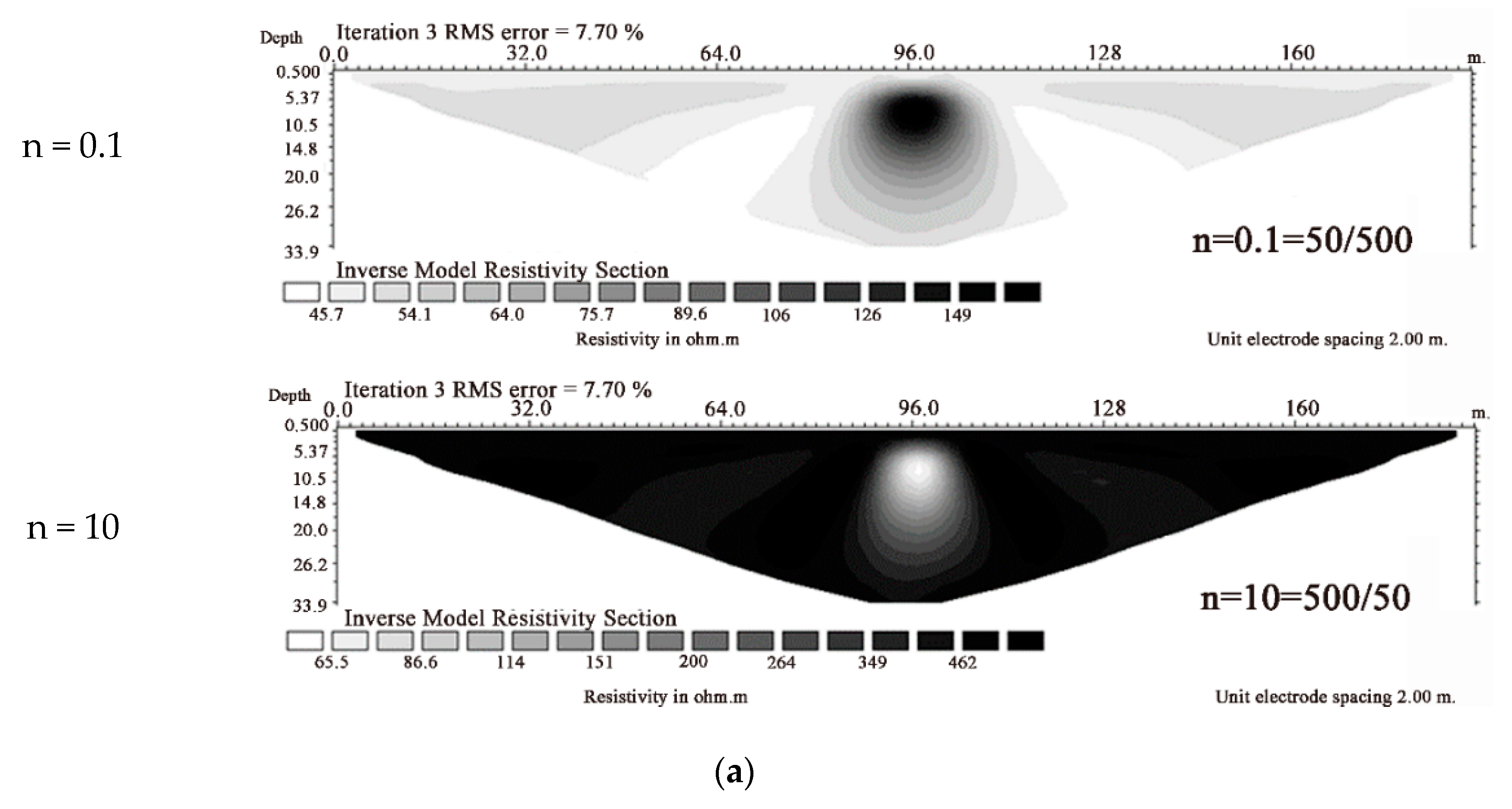
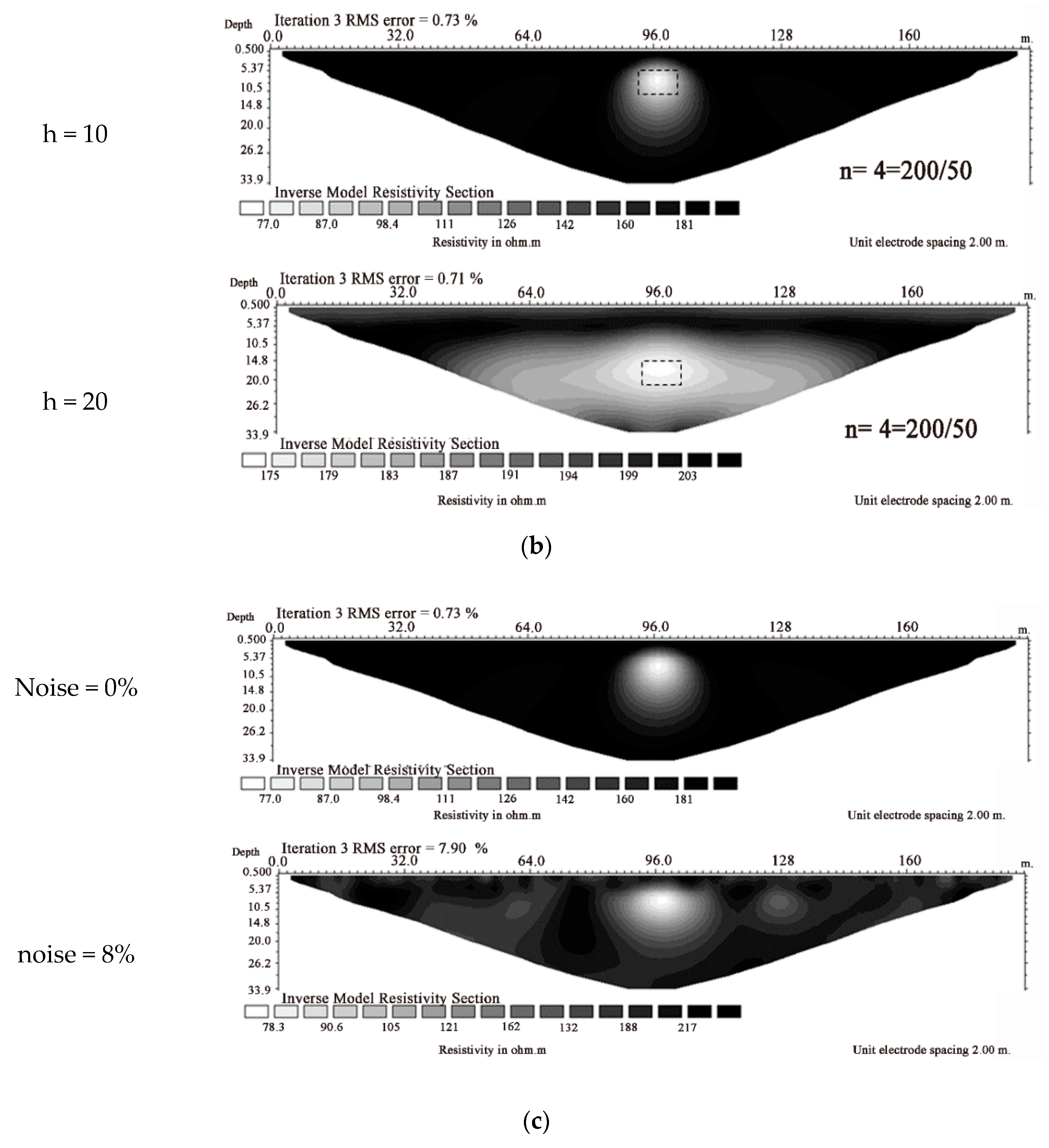
4.5. Composite Stratum Model

The results of Composite Stratum as shown in Figure 15. If there was a single material in the stratum, the material in the stratum, no matter if it had high or low resistance, could be identified clearly, but the identifiable depth of the material was influenced by the resistivity ratio. In the case of relatively high resistance material, the closer the R1 was to the R2 value, the material was lower than the set value. In the case of relatively low resistance material, the closer the R1 was to the R2 value, the detected area of the material was larger than the set value, as shown in Figure 15a. When the material center position descended, as the gradation zone expanded the material was still identifiable, but obscure, as shown in Figure 15b. When there was noise interference in the detection process, the resistivity profile had a random jump; the random jump worsened as the noise increased, and the area of material varied with the noise intensity, as shown in Figure 15c.

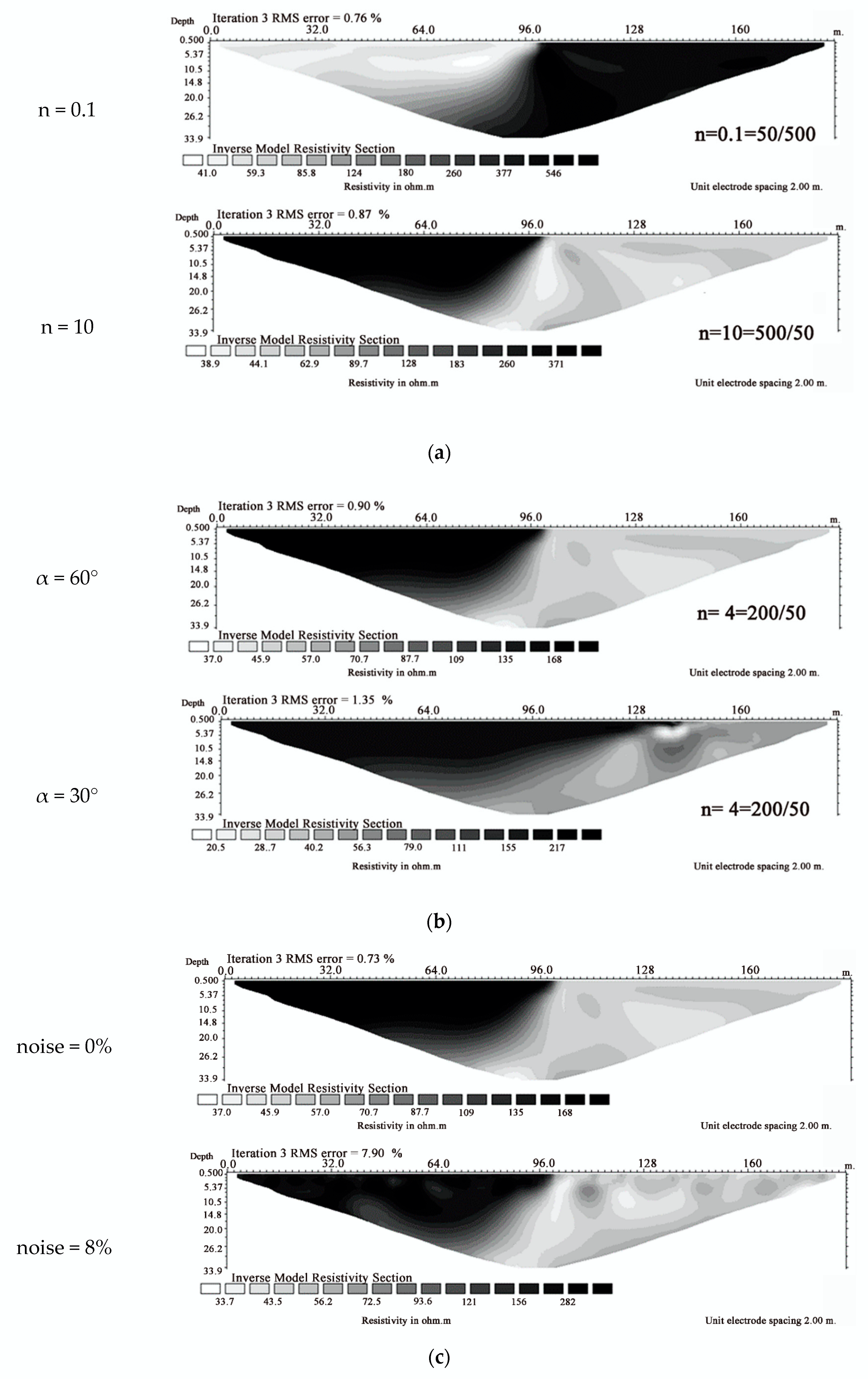
4.6. Tilted Layer Stratum Model

The results of Tilted Layer Stratum as shown in Figure 16. In the tilted layer stratum, when the upper layer had relatively low resistance, the tilted layer was unlikely to be identified. When the upper layer had relatively high resistance, the larger the difference between R1 and R2, the more obvious was the tilted layer, as shown in Figure 16a. When the tilt angle decreased, the tilted layer was more identifiable. However, when the upper layer had relatively low resistance, the deeper part was less likely to be identified, as shown in Figure 16b. When there was noise interference in the measurement process, the profile had jumping phenomena. When the upper layer had relatively low resistance, the tilted layer almost turned into a vertical layer as the noise increased, as shown in Figure 16c.

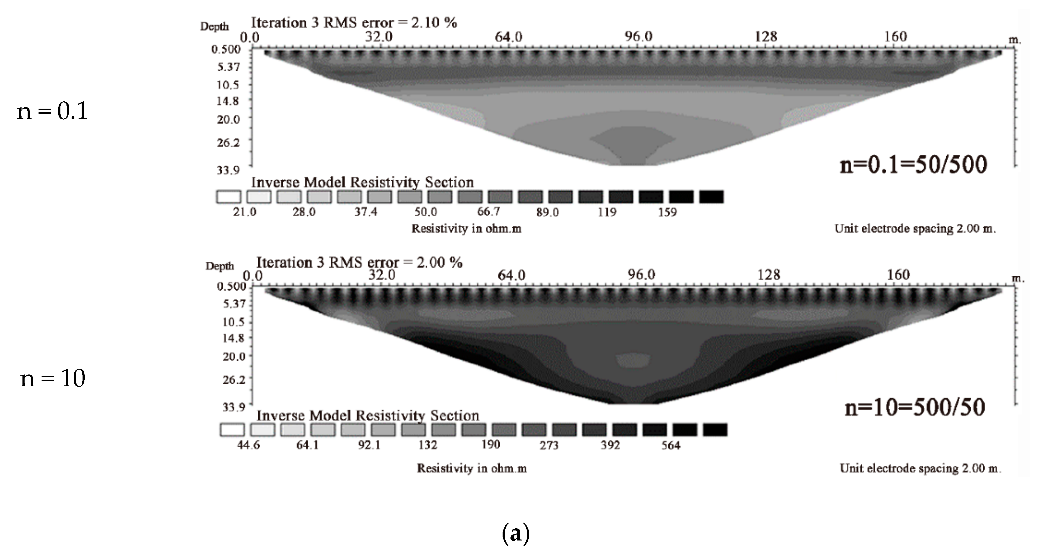
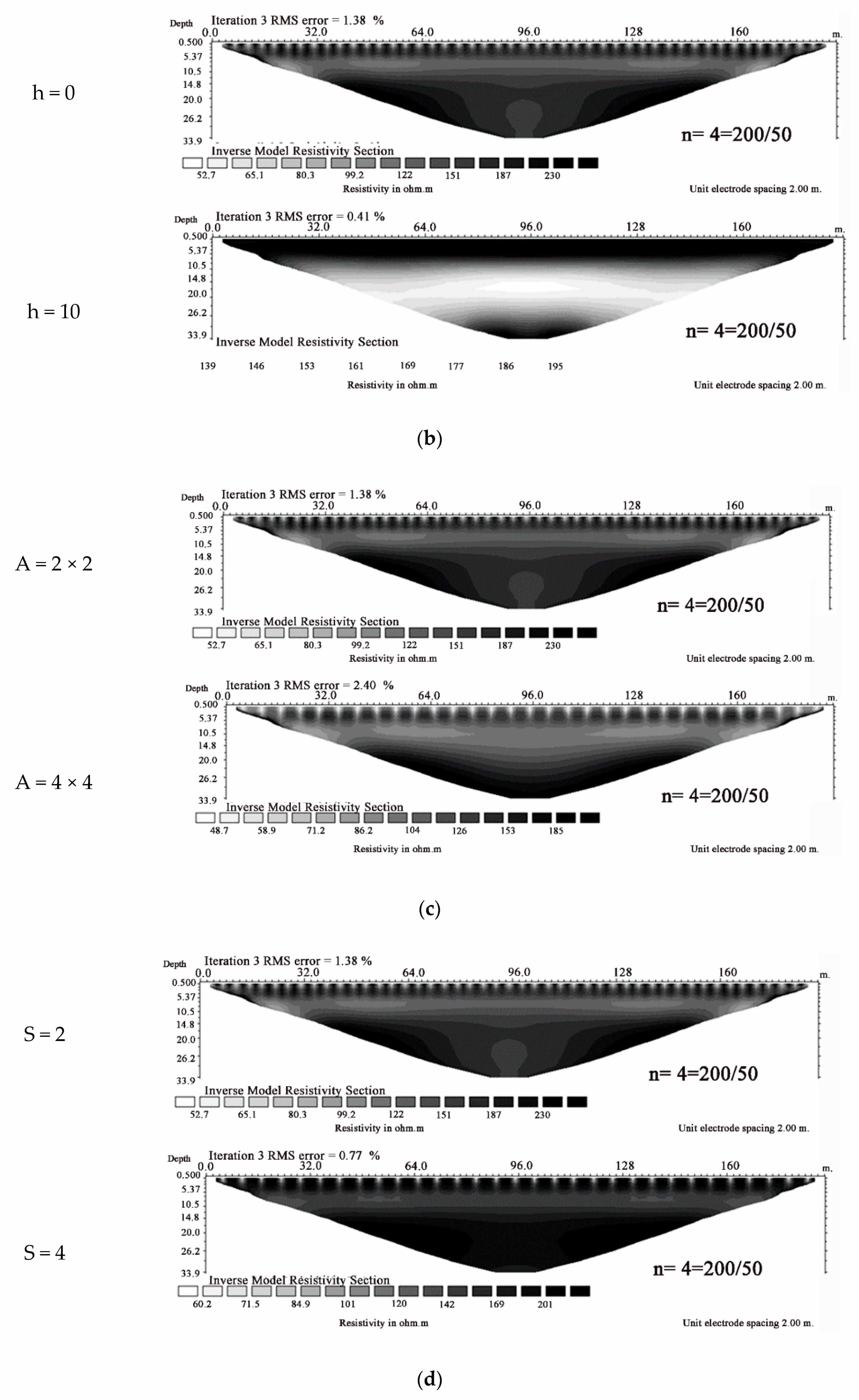
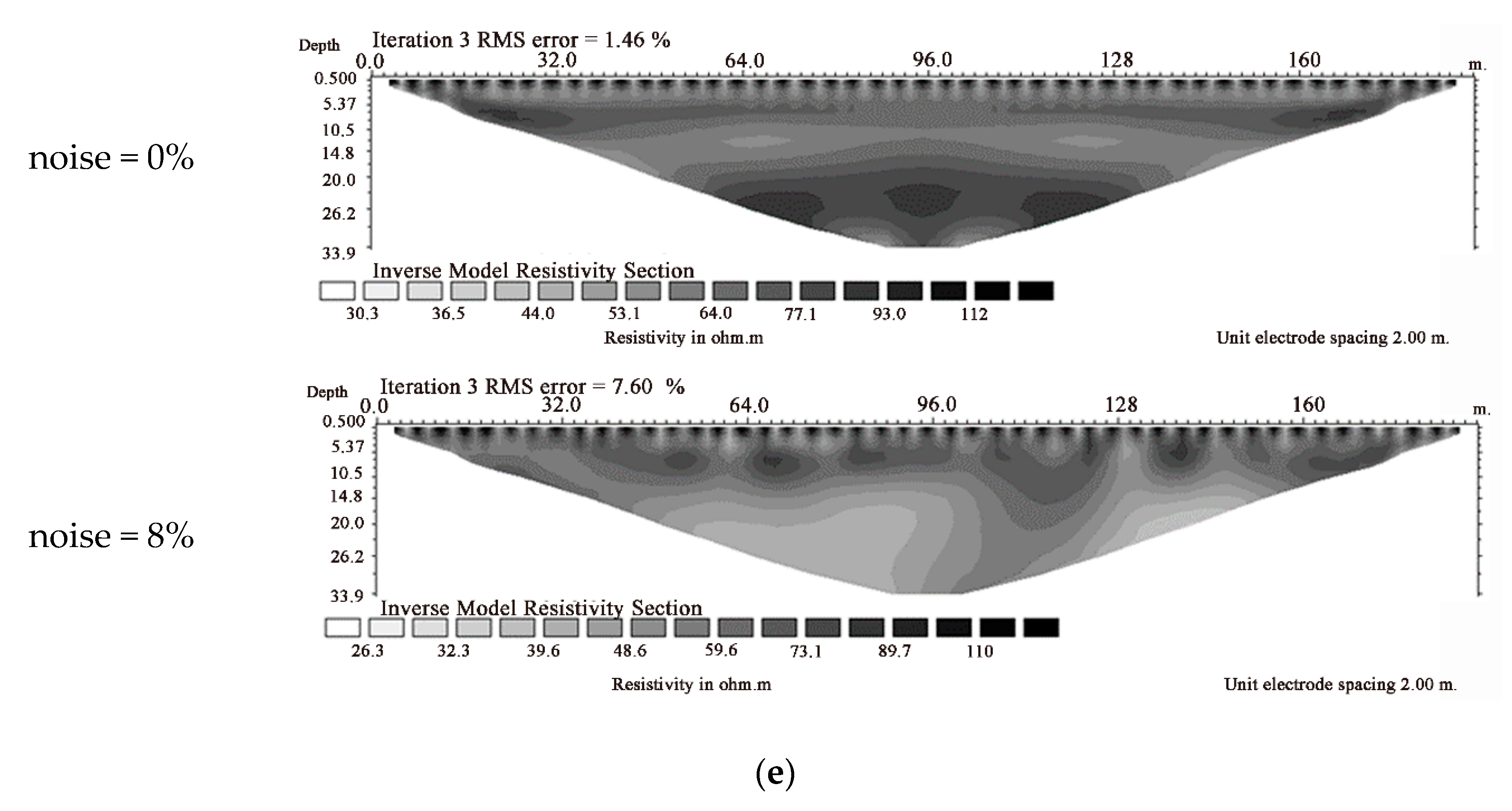
4.7. Debris Mixed Stratum Model

The results of Debris Mixed Stratum as shown in Figure 17. If there were multiple materials in the stratum, such as debris mixed stratum, the materials of Layer 1 could be identified clearly. The materials after Layer 2 were fuzzified and presented in zones. When the medium had relatively high resistance, the resistivity of the first layer of the medium was lower than the set value, and the resistivity decreased as the difference between the R1 and R2 values increased. When the background soil layer had relatively high resistance, the profile variation was more obvious as the difference between the R1 and R2 values increased, as shown in Figure 17a. When the covering depth increased, the deep medium was completely unidentifiable, as shown in Figure 17b. When the mesh area was enlarged, the resolution capability of the first layer of the medium was better, but the medium after Layer 1 was unidentifiable, as shown in Figure 17c. When the mesh spacing increased, the resolution capability of the first layer of the medium was better, but the medium after Layer 1 was unidentifiable, as shown in Figure 17d. When there was noise interference in the detection process, the resistivity profile had a random jump; the random jump worsened as the noise increased. The first layer of the medium was still identifiable, but the profile of the medium after Layer 1 was distorted, as shown in Figure 17e.

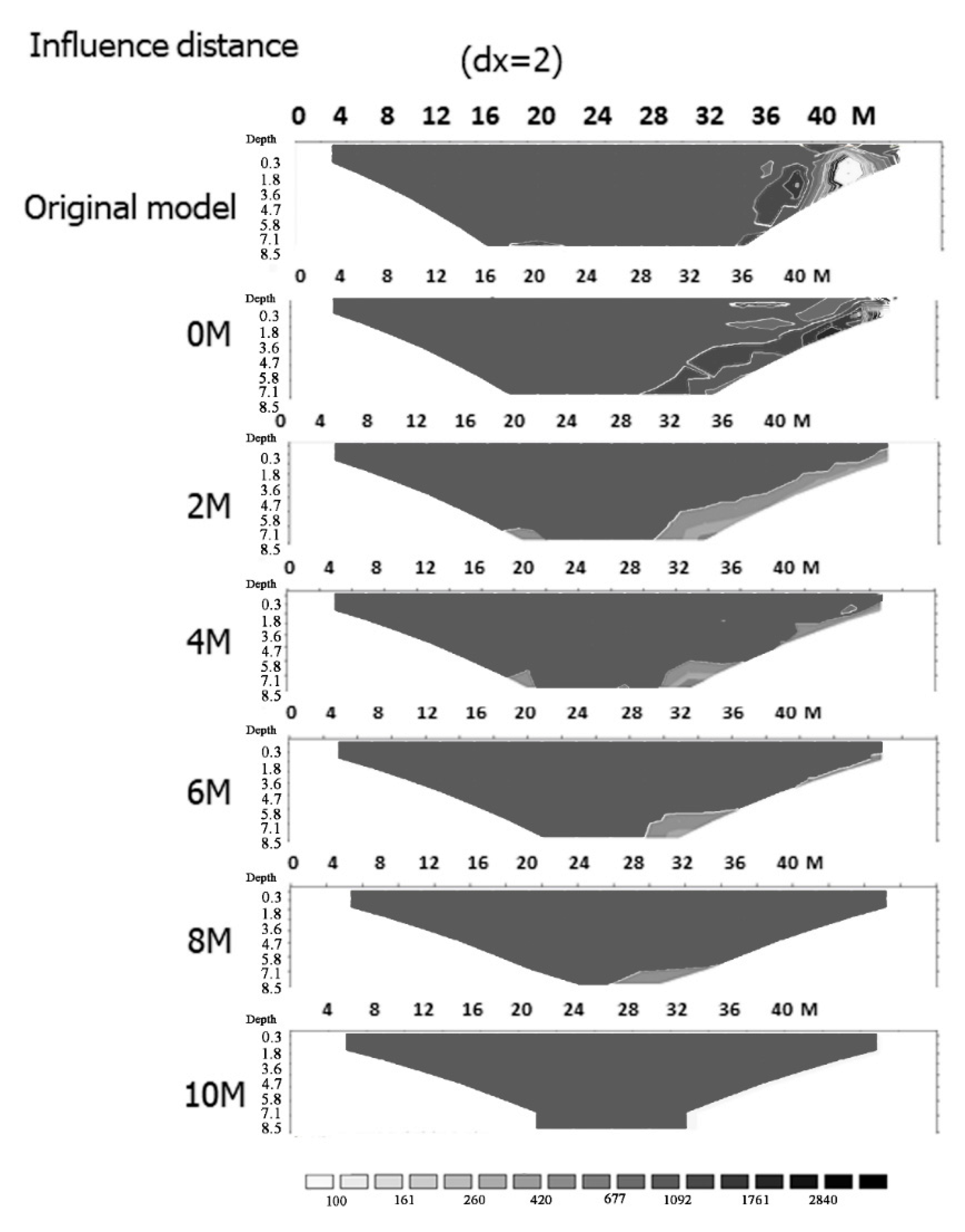
4.8. Influential Distances of the Boundary Effect

In order to know the range of influence of the boundary effect, the data of pipeline boundary distances of 0, 2, 4, 6, 8, and 10 m were deleted for inverse computation, and the model changed at the different distances observed; the results are shown in Figure 18. The resistivity profile charts within 6 m from the boundary medium had significantly abnormal electrical resistivity regions, and the boundary effect was apparent; when the distance to the boundary medium was 8 m, the boundary effect had little influence.

4.9. Influential Distances of the 3D Effect

In order to know the range of influence of the 3D effect, this study laid measuring lines L1–L5, which were 1.5, 0, 3, 6, and 9 m away from the pipeline boundary, respectively. The model changed at the different distances observed; the results are shown in Figure 19. The L1 and L3 profiles had an apparent 3D effect. The 3D effect was unclear gradually in the L4 measuring line profile. The 3D effect disappeared in the L5 measuring line profile. Therefore, the influential distance of the 3D effect was about 6m; the mapping phenomenon after 6 m weakened gradually. This result is similar to the influential distance of the boundary effect.

5. Conclusions and Suggestions

5.1. Conclusions

The electrical resistivity profile varies with strata, so this study built seven common geological models, including the single horizontal layer stratum, horizontal interlayer stratum, single vertical layer stratum, vertical interlayer stratum, composite stratum, tilted layer stratum, and debris mixed stratum, and used a Wenner array to arrange the electrodes. The findings show that besides the depth, the resolution capability of 2D electrical resistivity profiles may be influenced by the resistivity ratio, layer depth, covering depth, interlayer thickness, tilt angle, medium size, and noise intensity in different strata. In a single horizontal stratum, as the current flowed in the lower resistivity layer, the relatively low resistance stratum usually had good resolution capability, whereas the relatively high resistance stratum was influenced by the relatively low resistance stratum; if it was in the lower layer of relatively low resistance, the resolution capability began to decline. In the horizontal interlayer stratum, the resistivity of relatively low resistance stratum was close to the set value. However, if the relatively high resistance stratum was in the interlayer and lower layer, under the effect of relatively low resistance stratum, the resistivity was lower than the set value, and it was difficult to identify the layer. In the tilted layer, the tilted layer was more obvious when the tilt angle decreased. However, when the relatively low resistance was in the upper layer, the tilted layer was blurred. On the contrary, when the relatively high resistance was in the upper layer, the tilted layer could be identified clearly. If there was homogeneous material in the strata, no matter whether the material in the strata had relatively high or low resistance, it could be identified, but the material identification depth was influenced by the resistivity ratio. If there were multiple materials in the strata, e.g., debris mixed stratum, the material of Layer 1 could be identified clearly, but the material after Layer 2 was influenced by the resistivity of the background soil layer, fuzzified and displayed in zones on the profile. If there was noise interference in the course of measurement, the resistivity profile had a random jump, and the jump worsened as the noise increased. The boundary effect and 3D effect had similar influential distances, which were 6–8 m. The above situation should be paid special attention to when interpreting electrical resistivity profile images so as to avoid misrecognition.

5.2. Suggestions

• In the measurements on field test sites, the results of this study can enhance researchers’ ability to interpret electrical resistivity profiles, but the field data of hydraulics, geology, and drilling of the site are still required, so as to evaluate the practical situation of the strata of the site accurately.
• According to the findings, the external factors can degrade the resolution capability of ERT. In order to provide correct electrical resistivity profiles, the inverse computation method can be discussed in the future to enhance the resolution capability.
• It is suggested to build a standard geophysical exploration test field in the future, so as to compare and check different investigation and test methods.
• The strata are usually heterogeneous, so it is often found in field measurements that when the strata are not homogeneous in the direction normal to the measuring line, there is a 3D effect. The topographical changes should be paid attention to during in-situ measurements.
• When laying the ground resistance measuring line, the changes in the landforms and reliefs on both sides should be evaded to avoid the boundary effect.

References

1. Lin, C.P.; Lin, C.H.; Wu, P.L.; Liu, H.C.; Hung, Y.C. Applications and challenges of near surface geophysicals in geotechnical engineering. Chin. J. Geophys. 2015, 58, 2664–2680. [Google Scholar]
2. Lin, C.H.; Lin, C.P.; Hung, Y.C.; Chung, C.C.; Wu, P.L.; Liu, H.C. Application of geophysical methods in a dam project: Life cycle perspective and Taiwan experience. J. Appl. Geophys. 2018, 158, 82–92. [Google Scholar] [CrossRef]
3. Geotechnical and Geotechnical Site Characterization. Available online: https://www5.unitn.it/Biblioteca/it/Web/EngibankFile/5892871.pdf (accessed on 25 June 2020).
4. Geophysical Survey System, Inc. Traning Notes; GSSI Press: Nashua, NH, USA, 1992. [Google Scholar]
5. Geophysical Survey Systems Inc. RADAN for Windows Version 5.0 User’s Manual; GSSI Press: Nashua, NH, USA, 2003; pp. 1–132. [Google Scholar]
6. Ribolini, A.; Bini, M.; Isola, I.; Coschino, F.; Baroni, C.; Salvatore, M.C.; Zanchetta, G.; Fornaciati, A. GPR versus geoarchaeological findings in a complex archaeological site (Badia Pozzeveri, Italy). Archaeol. Prospect. 2017, 24, 141–156. [Google Scholar] [CrossRef]
7. Lee, D.H.; Lai, S.L.; Wu, J.H.; Chang, S.K.; Dong, Y.M. Detecting the remaining structure foundation using ground penetrating radar: The outer wall of small east gate of Taiwan-FU, Taiwan. J. Geoengin. 2018, 13, 85–92. [Google Scholar] [CrossRef]
8. Dahlin, T. The development of DC resistivity imaging techniques. Comput. Geosci. 2001, 27, 1019–1029. [Google Scholar] [CrossRef] [Green Version]
9. Beresnev, I.A.; Hruby, C.E.; Davis, C.A. The use of multi-electrode resistivity imaging in gravel prospecting. J. Appl. Geophys. 2002, 49, 245–254. [Google Scholar] [CrossRef]
10. Berternann, D.; Schwarz, H. Bulk density and water content-dependent electrical resistivity analyses of different soil classes on a laboratory scale. Environ. Earth Sci. 2018, 77, 570. [Google Scholar] [CrossRef]
11. Suzuki, K.; Toda, S.; Kusunoki, K.; Fujimitsu, Y.; Mogi, T.; Jomori, A. Case studies of electrical and electromagnetic methods applied to mapping active faults beneath the thick quaternary. Eng. Geol. 2000, 56, 29–45. [Google Scholar] [CrossRef]
12. Demanet, D.; Renardy, F.; Vanneste, K.; Jongmans, D.; Camelbeeck, T.; Meghraoui, M. The use of geophysical prospecting for imaging active faults in the Roer Graben, Belgium. Geophysics 2001, 66, 78–89. [Google Scholar] [CrossRef]
13. Batayneh, A.; Barjous, M. A Case Study of Dipole-Dipole Resistivity for Geotechnical Engineering from the Ras en Naqab Area, South Jordan. JEEG 2003, 8, 31–38. [Google Scholar] [CrossRef]
14. Rizzoa, E.; Colellab, A.; Lapennaa, V.; Piscitellia, S. High-resolution images of the fault-controlled High Agri Valley basin (Southern Italy) with deep and shallow electrical resistivity tomographies. Phys. Chem. Earth Parts A/B/C 2004, 29, 321–327. [Google Scholar] [CrossRef]
15. Nguyen, F.; Garambois, S.; Jongmans, D.; Pirard, E.; Loke, M.H. Image processing of 2D resistivity data for imaging faults. J. Appl. Geophys. 2005, 57, 260–277. [Google Scholar] [CrossRef]
16. Chen, Y.-P. Using RIP Method in Surveying Hsincheng Fault. Master’s Thesis, National Central University, Taoyuan, Taiwan, 2001. [Google Scholar]
17. Pan, H.-C. Using RIP Method in Surveying Hsinchu Fault. Master’s Thesis, National Central University, Taoyuan, Taiwan, 2003. [Google Scholar]
18. Griffiths, D.H.; Barker, R.D. Two-dimensional resistivity imaging and modelling in areas of complex geology. J. Appl. Geophys. 1993, 29, 211–226. [Google Scholar] [CrossRef]
19. Reci, H.; Muceku, Y.; Jata, I. The Use of ERT for Investigation of Berzhita Landslide, Tirana Area, Albania, Landslides and Monitoring; Springer: Berlin/Heidelberg, Germany, 2013; pp. 117–123. [Google Scholar]
20. Havevith, H.-B.; Jongmans, D.; Abdrakhmatov, K.; Trefois, P.; Delvaux, D.; Torgoe, I.A. Geophysical Investigations Of Seismically Induced Surface Effects: Case Study Of A Landslide In The Suusamyr Valley, Kyrgyzstan. Surv. Geophys. 2000, 21, 351–370. [Google Scholar] [CrossRef]
21. Giano, S.I.; Lapenna, V.; Piscitelli, S.; Schiattarella, M. Electrical imaging and self-potential survayes to study the geological setting of the Quaternary, slope depositsin the Agri high valley (Southern Italy). Ann. Geophys. 2000, 43. [Google Scholar] [CrossRef]
22. Godio, A.; Bottino, G. Electrical and electromagnetic investigation for landslide characterization. Phys. Chem. Earth Part C Solar Terr. Planet. Sci. 2001, 26, 705–710. [Google Scholar]
23. Batayneh, A.; Al-Diabat, A.A. Application of a two-dimensional electrical tomography technique for investigating landslides along the Amman–Dead Sea highway, Jordan. Environ. Geol. 2002, 42, 399–403. [Google Scholar] [CrossRef]
24. Perronea, A.; Iannuzzia, A.; Lapennaa, V.; Lorenzob, P.; Piscitellia, S.; Rizzoa, E.; Sdaob, F. High-resolution e lectrical imaging of the Varco d’Izzo earthflow (southern Italy). J. Appl. Geophys. 2004, 56, 17–29. [Google Scholar] [CrossRef]
25. Dahlin, T.; Glatz, D.; Persson, N.; Gwaze, P.; Owen, R. Electrical and Magnetic Investigations of Deep Aquifers in North Matabeleland, Zimbabwe. In Proceedings of the Fifth Meetingon Environmental and Engineering Geophysics, Budapest, Hungary, 5–9 September 1999; p. 2. [Google Scholar]
26. Kura, N.U.; Ramli, M.F.; Ibrahim, S.; Sulaiman, W.N.A.; Zaudi, M.A.; Aris, A.Z. A Preliminary Appraisal of the Effect of Pumping on Seawater Intrusion and Upconing in a Small Tropical Island Using 2D Resistivity Technique. Sci. World J. 2014, 2014, 796425. [Google Scholar] [CrossRef] [Green Version]
27. Oueuemi, K.D.; Aizebeokhai, A.P.; Oladunjoye, M.A. Integrated Geophysical and Geochemical Investigations of Saline Water Intrusion in a Coastal Alluvial Terrain, Southwestern Nigeria. Int. J. Appl. Environ. Sci. 2015, 10, 1275–1288. [Google Scholar]
28. Goebel, M.; Pidlisecky, A. Rosemary Knight, Resistivity imaging reveals complex pattern of saltwater intrusion along Monterey coast. J. Hydrol. 2017, 551, 746–755. [Google Scholar] [CrossRef]
29. Chen, T.T.; Hung, Y.C.; Hsueh, M.W.; Yeh, Y.H.; Weng, K.W. Evaluating the Application of Electrical Resistivity Tomography for Investigating Seawater Intrusion. Electronics 2018, 7, 107. [Google Scholar] [CrossRef] [Green Version]
30. Voronkov, O.K.; Kagan, A.A.; Krivonogova, N.F.; Glagovsky, V.B.; Prokopovich, V.S. Geophysical Methods and Identification of Embankment Dam Parameters. In Proceedings of the ISC-2 on Geotechnical and Geophysical Site Characterization, Porto, Portugal, 19–22 September 2004; pp. 593–599. [Google Scholar]
31. Song, S.H.; Song, Y.; Kwon, B.D. Application of hydrogeological and geophysical methods to delineate leakage pathways in an earth fill dam. Explor. Geophys. 2005, 36, 92–96. [Google Scholar] [CrossRef]
32. Oh, Y.C.; Jeong, H.S.; Lee, Y.K.; Shon, H. Safety Evaluation of Rock-Fill dam by Seismic (MASW) and Resistivity Method. In 16th EEGS Symposium on the Application of Geophysics to Engineering and Environmental Problems; European Association of Geoscientists & Engineers: Houten, The Netherlands, 2003; pp. 1377–1386. [Google Scholar]
33. Lin, C.P.; Hung, Y.C.; Wu, P.L.; Yu, Z.H. Performance of 2D ERT in Investigation of Abnormal Seepage: A Case Study at the Hsin-Shan Earth Dam in Taiwan. J. Environ. Eng. Geophys. 2013, 13, 101–112. [Google Scholar]
34. Darilek, G.T.; Corapcioglu, M.Y.; Yeung, A.T. Sealing Leaks in Geomembrane Liners Using Electrophoresis. J. Environ. Eng. 1996. [Google Scholar] [CrossRef]
35. Ramirez, A.; Daily, W.; Binley, A.; LaBrecque, D.; Roelant, D. Detection of Leaks in Underground Storage Tanks Using Electrical Resistance Methods. J. Environ. Eng. Geophys. 1996, 1, 189–203. [Google Scholar] [CrossRef]
36. Binley, A.; Daily, W.; Ramirez, A. Detecting Leaks from Environmental Barriers using Electrical Current Imaging. J. Environ. Eng. Geophys. 1997, 2, 11–19. [Google Scholar] [CrossRef]
37. Colucci, P.; Darilek, G.T.; Laine, D.L.; Binley, A. Locating Landfill Leaks Covered with Waste. In Proceedings of the International waste management and landfill symposium, Sardinia 99, Cagliari, Italy, 4–8 October 1999; Volume 3, pp. 137–140. [Google Scholar]
38. Daily, W.; Ramirez, A.; Binley, A. Remote Monitoring of Leaks in Storage Tanks using Electrical Resistance Tomography: Application at the Hanford Site. J. Environ. Eng. Geophys. 2004, 9, 11–24. [Google Scholar] [CrossRef]
39. Reci, H.; Jata, I.; Bushati, S. Ert method for the detection of buried archaeological objects in apollonia & bylis, Albania. Rom. Rep. Phys. 2015, 67, 665–672. [Google Scholar]
40. Cozzolino, M.; di Giovanni, E.; Mauriello, P.; Desideri, A.; Patella, D. Resistivity Tomography in the Park of Pratolino at Vaglia (Florence, Italy). Archaeol. Prospect. 2012, 19, 253–260. [Google Scholar] [CrossRef]
41. Loke, M.H.; Barker, R.D. Practical techniques for 3D resistivity surveys and data inversion techniques. Geophys. Prospect. 1996, 44, 499–524. [Google Scholar] [CrossRef]
42. Oldenborger, G.A.; Routh, P.S. The point-spread function measure of resolution for the 3D electrical resistivity experiment. Geophys. J. Int. 2009, 176, 405–414. [Google Scholar] [CrossRef] [Green Version]
43. Yang, X.; Lagmanson, M. Comparison of 2D and 3D Electrical Resistivity Imaging Methons. Adv. Geosci. 2006. [Google Scholar] [CrossRef]
44. Hung, Y.C.; Lin, C.P.; Lee, C.T.; Weng, K.W. 3D and Boundary Effects on 2D Electrical Resistivity Tomography. Appl. Sci. 2019, 9, 2963. [Google Scholar] [CrossRef] [Green Version]
45. Loke, M.H. Tutorial: 2-D and 3-D Electrical Imaging Surveys; Geotomo Software: Penang, Malaysia, 2004. [Google Scholar]
46. Griffiths, D.H.; Turnbull, J.; Olayinka, A.I. Two dimensional resistivity mapping with a computer-controlled array. First Break 1990, 8, 121–129. [Google Scholar] [CrossRef]
47. Geotomo Software 2002. RES2DMOD Ver. 3.01, Rapid 2D Resistivity forward Modelling Using the Finite-Difference and Finite-Element Methods. Available online: www.geoelectrical.com (accessed on 25 June 2020).
48. Geotomo Software 2007. RES2DINV Ver. 3.56, Rapid 2-D Resistivity and IP Inversion Using the Least-Squares Method. Available online: www.geoelectrical.com (accessed on 25 June 2020).
Figure 1. Method of 2D ERT: (a) Schematic diagram of the arrangement of current electrodes and potential electrodes and (b) 2D ERT measurement method and pseudo-section.
Applsci 10 04394 g001
Figure 2. Schematic diagram of the single horizontal layer stratum model.
Applsci 10 04394 g002
Figure 3. Schematic diagram of the horizontal interlayer stratum model.
Applsci 10 04394 g003
Figure 4. Schematic diagram of the single vertical layer stratum model.
Applsci 10 04394 g004
Figure 5. Schematic diagram of the vertical interlayer stratum model.
Applsci 10 04394 g005
Figure 6. Schematic diagram of the composite stratum model.
Applsci 10 04394 g006
Figure 7. Schematic diagram of the tilted layer stratum model.
Applsci 10 04394 g007
Figure 8. Schematic diagram of the debris mixed stratum model.
Applsci 10 04394 g008
Figure 9. Schematic diagram of the boundary effect model.
Applsci 10 04394 g009
Figure 10. Schematic diagram of the 3D effect model.
Applsci 10 04394 g010
Figure 11. Results of Single Horizontal Layer Stratum: (a) different resistivities, (b) layers at different heights, and (c) different noises.
Applsci 10 04394 g011aApplsci 10 04394 g011b
Figure 12. Results of horizontal interlayer stratum: (a) different resistivities, (b) interlayer center at different depths, (c) different interlayer thicknesses, and (d) different noises.
Applsci 10 04394 g012aApplsci 10 04394 g012b
Figure 13. Results of the single vertical layer stratum: (a) different resistivities and (b) differen noises.
Applsci 10 04394 g013
Figure 14. Results of the vertical interlayer stratum: (a) different resistivities, (b) different interlayer thicknesses, and (c) different noises.
Applsci 10 04394 g014aApplsci 10 04394 g014b
Figure 15. Results of composite stratum: (a) different resistivities, (b) different material center depths, and (c) different noises.
Applsci 10 04394 g015aApplsci 10 04394 g015b
Figure 16. Results of Tilted Layer Stratum: (a) different resistivities, (b) different tilt angles, and (c) different noises.
Applsci 10 04394 g016
Figure 17. Results of debris mixed stratum: (a) different resistivities, (b) different covering depths, (c) different mesh sizes, (d) different mesh spacings, and (e) different noises.
Applsci 10 04394 g017aApplsci 10 04394 g017bApplsci 10 04394 g017c
Figure 18. Influential distances of the boundary effect.
Applsci 10 04394 g018
Figure 19. Influential distances of the boundary effect.
Applsci 10 04394 g019