Similarity Analysis for Time Series-Based 2D Temperature Measurement of Engine Exhaust Gas in TDLAT

Abstract

As regulations on the emission of pollutants from combustion systems are further tightened, it is necessary to reduce pollutant species and improve combustion efficiency to completely understand the process in the combustion field. Tunable diode laser absorption tomography (TDLAT) is a powerful tool that can analyze two-dimensional (2D) temperature and species concentration with fast-response and non-contact. In this study, stabilized spectra were implemented using the mean periodic signal technique to enable real-time 2D temperature measurement in harsh conditions. A time series statistical-based verification algorithm was introduced to select an optimal spectral cycle to track 2D reconstruction temperature. The statistical-based verification is based on the Two-sample t test, root mean square error, and time-based Mahalanobis distance, which is a technique for similarity analysis between thermocouple and reconstruction temperature of 18 candidate cycles. As a result, it was observed that the statistical-based TDLAT contribute to improving the accuracy of time series-based 2D temperature measurements.

1. Introduction

With global warming prevention and environmental protection emerging as an issue all over the world, emission regulations are gradually being tightened as the effects of emissions from combustion systems on air and human bodies are highlighted. For example, EURO 6 regulations are an effort to reduce emissions such as CO, HC, NO_x, and PM by the auto industry. The recent EURO 6d emission regulations require real driving emissions (RDE) tests, which measure pollutants emitted from motor vehicles while they are driven, as an additional approval. As a result, demand for vehicles with low NO_x emissions and high engine power has increased, and several studies have been conducted to improve the performance of NO_x after treatment systems [1,2,3]. An important element in catalytic after treatment devices is exhaust gas temperature because catalytic performance is a function of temperature. A car engine running at high temperature tends to emit less CO₂ and more NO_x. On the other hand, a lower engine temperature will result in more CO₂ and less NO_x. However, the challenge of reducing both CO₂ and pollutant emissions simultaneously still remains. Therefore, analysis of temperature and species concentration during combustion is necessary for fundamental understanding of combustion reaction, which may reduce pollutants in the combustion system and improve combustion efficiency. However, the thermocouple (TC), a conventionally used one-point temperature measurement device, has difficulty in analyzing non-uniform flow, such as in engine exhaust. In addition, the techniques such as coherent anti-stokes Raman scattering (CARS) [4,5] and laser induced grating spectroscopy (LIGS) [6], which are recently used in the spectroscopy field, can measure temperature at a fast response speed, but have a limit of point measurement, and filtered Rayleigh scattering (FRS) [7] and planer laser induced fluorescence (PLIF) [8,9] enable two-dimensional temperature, but their measurement systems are expensive and complicated. Tunable diode laser absorption tomography (TDLAT) is a suitable tool for understanding the combustion process by allowing 2D analysis of temperature and species concentration with non-contact fast-response. Therefore, it has been developed with various TDLAT techniques for measuring 2D temperature and species concentration in combustion fields [10,11,12,13,14]. Deguchi et al. demonstrated a 2D temperature distribution measurement by TDLAT on Bunsen-type flame burners and gasoline engines [10]. Ma et al. developed a hyperspectral tomography (HT) method that can simultaneously measure 2D distribution of temperature and H₂O concentration with a temporal resolution of 50 kHz at the exhaust plane of a j85 engine [11]. Busa et al. developed a measurement method of combustion efficiency that combines TDLAT and particle image velocimetry (PIV) in the scramjet engine [13]. However, these methods cannot be applied directly for real-time measurements because of excessive computational time and lack of time resolution assessment required for computed tomography (CT) analysis.

This study introduced a spectral cycle parameter improving reconstruction performance with a posteriori statistical technique in conventional absorption tomography to measure the exhaust gas temperature in milliseconds through TDLAT. Signal stabilization technique was applied in various cycle models to obtain stabilized absorption spectra in harsh environments, and statistical verification using TC measurement was performed to evaluate the results of the time series 2D reconstruction temperature distribution.

2. Theory of TDLAS

Tunable diode laser absorption spectroscopy (TDLAS) is a measurement technique commonly used in a variety of applications recently as well as temperature and density of molecules in gas [15,16]. When a laser beam permeates an absorption medium, its intensity will be attenuated by the absorbing gas species. This phenomenon is measured by TDLAS system that continuously scans laser wavelengths. The principle of TDLAS is theoretically expressed in terms of absorption by Beer-Lambert law that describes the relationship between the incident intensity I_v0 and transmitted intensity I_v as follows:

$$\frac{I_v}{ I_{v0}}=exp\left\{-A_v\right\}=exp\left\{-{{\displaystyle \int }}_0^L{\alpha }_v\left(s\right)ds\right\},$$

(1)

where $A_{\nu }$ denotes the spectral absorbance of representative wavenumber $\mathsf{\nu }$. L denotes the optical path length, and ${\alpha }_{\nu }$ is the local mass-weighted absorption coefficient at position s along the laser beam, from 0 to L. This quantity is given by the following expression:

$${\alpha }_v={\displaystyle \sum }_i\frac{x_{i}p}{kT}{\displaystyle \sum }_j{S}_{i,j}\left(T\right){ƒ}_v\left(v;v_j,\Delta {\nu }_G,\Delta {\nu }_L \right),$$

(2)

where, k [J/K] denotes Boltzmann’s constant, ${ƒ}_v$ is the Voigt profile, with Lorentzian and Gaussian half width at half maximums (HWHMs), $\Delta {\nu }_L$ and $\Delta {\nu }_G$ [17,18,19]. p denotes pressure, assumed to be uniform and x_i denotes mole-fraction of absorbing species i, where, $x_i$, p, and T are evaluated locally. S_i,j(T) denotes temperature dependent line strength of absorption transition j and can be calculated by a function of temperature as follows:

$$S_{i,j}\left(T\right)=S_{i,j}\left(T_0\right)\frac{Q\left(T_0\right)}{Q\left(T\right)}\frac{T}{T_0}exp\left[-\frac{hc{E}_i^{″}}{k}\left(\frac{1}{T}-\frac{1}{T_0}\right)\right]\left[1-exp\left(\frac{-hc{v}_{0,i}}{kT}\right)\right]{\left[1-exp\left(\frac{-hc{v}_{0,i}}{k{T}_0}\right)\right]}^{-1},$$

(3)

where, h (J·s) and c (cm/s) denote Planck’s constant and the speed of light, v₀ (cm⁻¹) denotes the line-center wavenumber, E_i″ (cm⁻¹) denotes lower-state energy of the transition, T₀ (K) is the reference temperature (296 K), and Q(T) denotes the partition function of molecular absorption at a particular temperature. It is usually expressed as a 4th order polynomial function [20]. Although it is difficult to accurately describe the chemical formula of gasoline, iso octane (C₈H₁₈) was selected because it is the hydrocarbon component with similar thermal properties to the actual composition. The combustion reaction of iso octane is as follows:

$$C_8{H}_{18}+ 12.05\left(O_2+3.76N_2\right)\to 8C{O}_2+ 9H_{2}O + 12.05·\left(3.76\right)N_2.$$

(4)

Among the combustion products, nitrogen (N₂) is an inert gas and hence, there is no chemical or absorption reaction. Therefore, water-vapor (H₂O) was chosen for exhaust gas diagnosis because of its high mole fraction and high absorption strength.

Figure 1 shows the theoretical H₂O absorption spectra calculated using the HITRAN2012 molecular spectroscopic database [21]. The patterns of the absorption spectra can be observed as the temperature changes. In this study, three peaks lines (7202.255 cm⁻¹, 7202.909 cm⁻¹, and 7203.891 cm⁻¹) with high line strengths and no interference with other molecules were chosen for calculating reconstruction temperature.

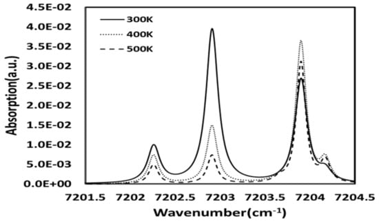
Figure 1. Theoretical H₂O absorption spectrum.

3. Experiment and Tomography Analysis

A schematic diagram of a TDLAS system measuring engine exhaust temperature is shown in Figure 2. The OHC (over head camshaft) gasoline engine (EX17, Subaru Robin, Doylestown, PA, USA) is driven in idle mode to produce emissions. The exhaust pipe installed 5 mm below the measurement cell was 20 mm in diameter and 150 mm in length. The distributed feedback (DFB) laser (NLK1E5GAAA, NTT Electronics, Japan) for H₂O gas target is tuned to the near-infrared spectral region at 1388 nm by a laser diode controller (LDC-3900, ILX Lightwave, Bozeman, MT, USA). The modulated laser beam is split into 16 channels by a 1 × 16 fiber optic coupler (SMF-28e, OPNETI, NY, USA). Among them, the 10 beams are irradiated into 10 collimators (50-1310-APC, THORLABS, Newton, NJ, USA) and the transmitted optical signals are detected by 10 photodetectors (G12180-010A, Hamamatsu Photonics, Japan). The received laser signals are amplified and filtered by low pass filters to remove signal noise. The amplified signals are transmitted into a data recorder (8861 Memory High Coda HD Analog16, HIOKI, Japan) in real time at a sampling rate of 500 kHz. Simultaneously, the real temperature for verification is measured by a B-type TC at the sampling rate of 1 kHz at the center of the target area. After absorption, signals collect by the data acquisition card are sent to the computer for reconstruction calculation.

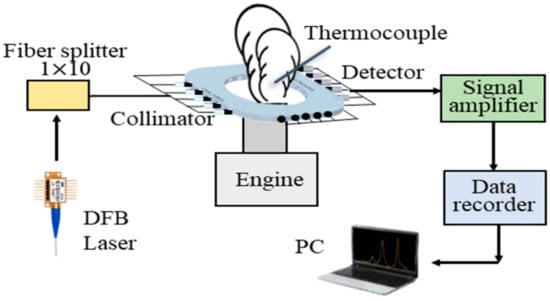
Figure 2. Schematic diagram of the experimental setup using tunable diode laser absorption spectroscopy (TDLAS).

Multiple parallel laser beams pass through the region of interest. The intersected spectral information is used to reconstruct 2D temperature by CT analysis. Figure 3 shows the laser paths and grids in the measurement region. The laser path consists of 10 real beams in a 5 × 5 layout and eight interpolated virtual beams The interpolated virtual beams imply the virtual signal data interpolated from the signal of the actual beam, and in the signal application field a widely introduced cubic spline interpolation is used in this study [22]. The cell length through which the laser passes in the measurement area is 60 mm and reconstruction area is 40 mm, and the spatial region for CT analysis consist of 81 (9 × 9) square grids with a grid size of 2.0 mm × 2.0 mm.

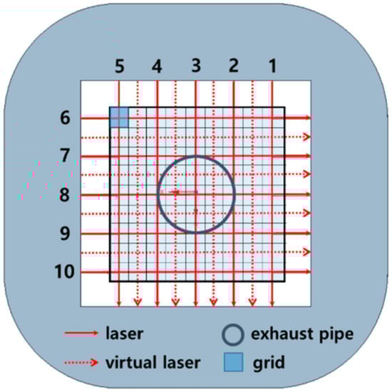
Figure 3. Laser paths and measurement cell.

Unexpected error signals due to harsh conditions were removed to reduce reconstruction calculation time for converging. The formula is as follows:

$${\delta }_t={\displaystyle \sum }_{n=1}^N\frac{{\left|{\overline{I}}_{v0,i}-{\overline{I}}_{v,i}\right|}_t}{ {\left|{\overline{I}}_{v0,i}-{\overline{I}}_{v,i}\right|}_{t-1}},$$

(5)

where, the subscript t denotes a cycle at t time and n denotes the data number in a cycle. $\delta$ denotes the error rate, which is a ratio of absolute error sum in ${\overline{I}}_v$ and ${\overline{I}}_{v0}$ of the cycle to that of the previous cycle. Here, the signal cycle was eliminated when ${\delta }_t$ is greater than 1.5. This method effectively reduced the error when converting the signal into the spectra. The noises generated by beam steering, window foul, and thermoelectric noises were approximated by Gaussian noise modeling, and the stabilized absorption spectra was obtained by the polynomial reduction method (PRM) averaging a number of absorption signal cycles [10,23,24] Although averaging a significant number of absorption cycles provides more stable signal, it has the drawback of degrading time-resolution and distorting raw signals. Hence, it is necessary to investigate appropriate number of cycles with good reconstruction performance and fast time-resolution simultaneously.

Figure 4 shows the result of mean transmitted signals (${\overline{I}}_v$) and mean absorption spectra using a total of 201 cycles (1 reference cycle, 100 cycles in front and 100 cycle in back) measured by the TDLAS system. Here, one cycle of measured signal consists of 500 samples with a recording time of 1 ms. A total of 5 million signals were received during 10 s of engine operation. Figure 4a is the result of averaging each raw signal acquired from the photodetector at the same time when 10 lasers passed through the target area. To convert these signals into absorption spectra, ${\overline{I}}_v$ and the mean incident signal (${\overline{I}}_{v0}$) must be known as shown in Equation (4). ${\overline{I}}_{v0}$, also known as the baseline, was estimated by PRM, which is a least squares fitting using 5th order polynomial curve with ${\overline{I}}_v$ [23,25]. To facilitate curve fitting, the saw-tooth waveform had a frequency of 1 kHz and a sampling rate of 2 μs. All measured absorption spectra generated from ${\overline{I}}_v$ and ${\overline{I}}_{v0}$ is shown in Figure 4b. These spectra consisted of 311 wavenumbers. Laser group 0 and 1 represent a group of vertical and horizontal lasers, respectively. The spectra pattern can be identified by different laser numbers. As shown in Figure 1, the measured absorption spectra are determined by the temperature of the measurement area, so the reconstructed temperature distribution in measurement zone can be traced by a tomographic reconstruction method from the information of each absorption spectrum.

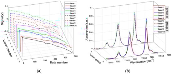
Figure 4. Results of mean transmission signals and mean absorption spectra of 10 laser beams: (a) 10 mean transmitted signals using 201 cycles and (b) 10 mean absorption spectra using 201 cycles.

The determination method of cycle and temperature is illustrated in Figure 5. First, raw absorption signals, reference time i and candidate cycle j are input. i denotes analysis time point at engine running time. A total of 990 absorption signals were used in 0.1 s from 1.0 to 9.9 s. j denotes the number of cycles of absorption signal to be averaged. Eighteen candidate cycles were chosen to evaluate the analytical performance in various cycles (31, 51, 71, 91, 111, 151, 201, 251, 301, 351, 401, 451, 501, 601, 701, 801, 901, and 1001 cycles).

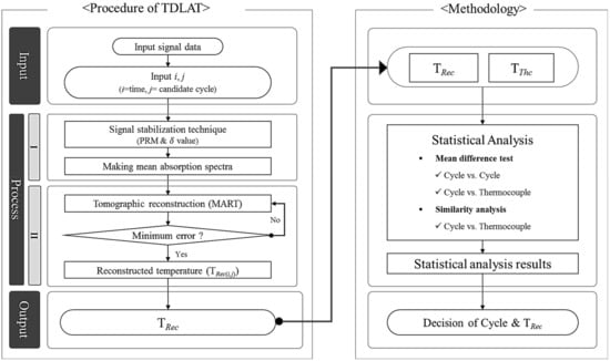
Figure 5. Flowchart for tracking cycle and reconstructed temperature using TDLAT.

In the second step, the PRM and $\delta$ value are combined to obtain mean absorption spectra, described in more detail above. This technique was able to remove noise more effectively than the conventional PRM. Reconstruction calculation consisting of 9 × 9 array was calculated using mean absorption spectra. The reconstructed temperature distribution was tracked by repeated calculations until errors in the experimental and theoretical absorption spectra were minimized by the multiplicative algebraic reconstruction technique (MART) algorithm [24].

$${\mathsf{\alpha }}_{v\left(\mathrm{n},\mathrm{m}\right)}{}^{\left(k\right)}={\mathsf{\alpha }}_{v\left(\mathrm{n},\mathrm{m}\right)}{}^{\left(k-1\right)}\times {\left[\frac{{\mathrm{A}}_v}{L_{\left(n,m\right)}{{\displaystyle \sum }}_{m=1}^M{{\displaystyle \sum }}_{n=1}^N{\mathsf{\alpha }}_{v\left(\mathrm{n},\mathrm{m}\right)}{}^{\left(k-1\right)}}\right]}^{\beta L_{\left(n,m\right)}},$$

(6)

where, the superscript k represents the number of iteration and the subscript (n, m) is the gird number. β is the relaxation parameter that affects the rate of convergence and was set to 0.1. The initial values of ${\mathsf{\alpha }}_{v\left(\mathrm{n},\mathrm{m}\right)}$ at each grid are an important factor for fast convergence calculation, which were approximated to target values by adopting the multiplication line of sight (MLOS) method [26]. The reconstruction calculation was terminated when difference of ${\mathsf{\alpha }}_{v\left(\mathrm{n},\mathrm{m}\right)}{}^{\left(k\right)}$ and ${\mathsf{\alpha }}_{v\left(\mathrm{n},\mathrm{m}\right)}{}^{\left(k-1\right)}$ was less than 1 × 10⁻⁶.

Figure 6 shows a comparison of the measured absorption spectra with the calculated absorption spectra in the engine running time of 5.0 s. The average root-mean-square error (RMSE) at 311 wavenumber were 9.766 × 10⁻⁴, 4.485 × 10⁻⁵, 1.273 × 10⁻³, and 2.144 × 10⁻³, respectively, in Figure 6a–d. Measured spectra were in good agreement with spectra by the theoretical calculation, but the measured spectra for the 51 and 201 cycles were slightly different from each other, and their reconstruction calculations were also differed slightly. This implies that the number of mean absorption cycles is an important parameter for the reconstruction results.

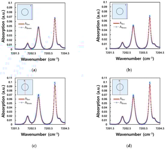
Figure 6. The spectra of reconstructed and measured absorption data at the engine running time 5.0 s: (a) 51 cycles, boundary; (b) 201 cycles, boundary; (c) 51 cycles, center; and (d) 201 cycles, center.

In the third step, the reconstructed temperatures, T_Rec(i,j), calculated for each candidate cycle and time are output. To estimate the T_Rec(i,j) from the finally converged ${\mathsf{\alpha }}_{v\left(\mathrm{n},\mathrm{m}\right)}$ at all grids, the theoretical absorption coefficients at the temperature has already been calculated using the HITRAN database for the mole fraction 1.0. The correlation between the theoretical absorption coefficient, ${\mathsf{\alpha }}_{v,the}$, and the reconstructed absorption coefficient, ${\mathsf{\alpha }}_v$, was evaluated to find the value with the most similar pattern, i.e., the nearest correlation coefficient to 1.0, and to obtain T_Rec(i,j). The correlation coefficient, $C_{n,m}$, at each grid is described as follows.

$$C_{n,m}=\frac{{{\displaystyle \sum }}_{v=1}^n\left({\mathsf{\alpha }}_v-\overline{\mathsf{\alpha }}\right)\left({\mathsf{\alpha }}_{v,the}-{\overline{\mathsf{\alpha }}}_{the}\right)}{\sqrt{{{\displaystyle \sum }}_{v=1}^n{({\mathsf{\alpha }}_v-\overline{\mathsf{\alpha }})}^2{{\displaystyle \sum }}_{v=1}^n{\left({\mathsf{\alpha }}_{v,the}-{\overline{\mathsf{\alpha }}}_{the}\right)}^2}},$$

(7)

where $\overline{\mathsf{\alpha }}$ and ${\overline{\mathsf{\alpha }}}_{the}$ denote the average value each of the theoretical and reconstructed absorption coefficient.

Figure 7 shows the results of 2D reconstructed temperature distribution using 51 and 201 cycles at the engine running time of 5.0 s. Comparing Figure 7a,b, the temperature difference at the center point was 12.35 K and the RMSE at all grids was 5.87 K. This is an example of the highest temperature difference compared to other engine running times. The characteristics of the temperature distribution for each time were similar, but the temperature fluctuation was shown differently. From these results, it was found that the number of mean cycles affected the results of CT analysis. Additionally, the output $\overline{T}$_Rec was set to the average value of nine grids located in the center of the measurement area as the TC was installed in the center of the exhaust pipe and the temperature was measured at one point. After all, the output T_Rec consists of a set of elements $\overline{T}$_Rec for each i and j. The number of T_Rec was 17820 in the i × j array (990 × 18).

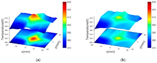
Figure 7. 2D reconstructed temperature distributions at the engine running time 5.0 s: (a) 51 cycles and (b) 201 cycles.

In the fourth step, the statistical-based analysis was performed using T_Rec and T_Thc, which means temperature measured by TC and was used to determine the cycle and T_Rec most similar to T_Thc. Further details are described in Section 4.

The computation time of each step on an Intel Core i7 2600K CPU with 16GB RAM was as follows. The CPU time of Process I to convert signal data into mean absorption spectra was 1.38 s and 1.90 s (311 wavenumbers) respectively at 51 and 201 cycles. As the number of mean cycles increased, the CPU time increased linearly. The CPU time of Process II was scored in under 1.79 s (311 wavenumbers), mostly converging on less than 150 iterations.

4. Statistical-Based Mean Difference Test and Similarity Analysis

The statistical-based analysis is performed to identify cycles that represent T_Rec similar to T_Thc. The 18 candidate cycles were selected using suitable intervals for analysis from 31 to 1001 cycles. The procedure is shown in Figure 8. Paired t test, which is a mean difference testing method, is conducted to evaluate the similarity between the 18 candidate cycles [27].

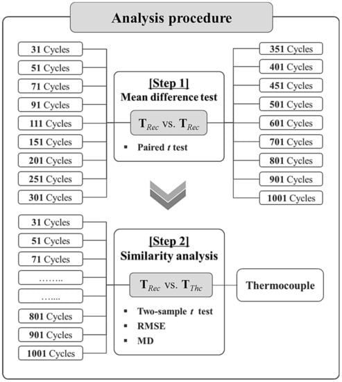
Figure 8. Procedure for mean different test and similarity analysis.

The next step is followed by performing a mean difference test and similarity analysis between T_Thc and T_Rec for all 18 candidate cycles. The mean difference test uses the representative statistical technique of Two-sample t test. RMSE and time-based Mahalanobis distance (TMD) were used for similarity analysis. RMSE is a measure of generalization of standard deviations that indicates the difference between actual and estimated values [28]. The Mahalanobis distance (MD) represents the distance between data and considers covariance [29].

Finally, the cycles that represent T_Rec most similar to T_Thc based on the analysis results were determined.

4.1. [Step 1] Mean Difference Test

T_Rec derived from 18 candidate cycles consists of 0.1 s intervals from 1 to 9.9 s as shown in Table 1. To test the mean temperature difference in 18 candidate cycles, the analysis was performed on nine T_Rec(i,j), which is the reconstructed temperature of ith reference time of the j-cycles. The total number of sets comparing T_Rec(i,j) in 18 candidate cycles to each other for the paired t test were 153. For the actual test, the analysis was performed only at the reference time (1 s, 2 s, 3 s, 4 s, 5 s, 6 s, 7 s, 8 s, and 9 s) for all 153 sets.

Table 1. T_Rec per 18 candidate cycles used in [Step 1].

No.	Time (s)	TRec
		31	51	$\cdots$	901	1001
1	1.0	404.833	400.000	$\cdots$	405.432	404.189
2		406.775	401.665	$\cdots$	407.081	405.842
3		404.947	399.784	$\cdots$	405.436	404.455
4		407.458	401.846	$\cdots$	407.028	405.633
5		409.400	403.506	$\cdots$	408.581	407.223
6		407.556	401.614	$\cdots$	406.820	405.720
7		404.951	399.982	$\cdots$	405.459	404.137
8		406.842	401.604	$\cdots$	406.900	405.606
9		404.999	399.722	$\cdots$	405.051	405.159
$\cdots$	$\cdots$	$\cdots$	$\cdots$	$\cdots$	$\cdots$	$\cdots$
806	9.9	398.712	399.182	$\cdots$	400.164	400.543
807		397.870	397.965	$\cdots$	402.270	402.782
808		396.147	396.544	$\cdots$	401.184	401.859
809		397.183	397.668	$\cdots$	401.351	401.646
810		396.221	396.327	$\cdots$	403.357	403.785

4.1.1. Paired t Test

The paired t-test is useful for analyzing the same set of items that were measured under two different conditions, i.e., differences in measurements made on the same subject before and after a treatment, or differences between two treatments given to the same subject.

The paired t-test is based on the test statistic as shown below:

$$T_{pt}=\frac{\overline{D}-d_0}{S_D/\sqrt{n}},$$

(8)

where,

$$\overline{D}=\frac{{{\displaystyle \sum }}_{k=1}^n\left(T_{Rec{\left(i,A\right)}^k}-T_{Rec{\left(i,B\right)}^k}\right)}{n},$$

(9)

$$S_D=\sqrt{\frac{{{\displaystyle \sum }}_{\mathrm{k}=1}^{\mathrm{n}}{\left(T_{Rec{\left(i,A\right)}^k-}{T}_{Rec{\left(i,B\right)}^k-}\overline{D}\right)}^2}{\mathrm{n}-1}},$$

(10)

where, $\overline{D}$ denotes the mean of the differences between the two kinds of cycles.$d_0$ denotes a constant that can be set depending on whether the mean of the difference between the two groups is zero or a specific non-zero value. $S_D$ denotes the standard deviation of differences between two kinds of cycles. T_Rec(i,A)^k denotes the kth reconstruction temperature at ith time (s) of cycle A, $i=1.0,1.1,1.2,\cdots ,9.9$. T_Rec(i,B)^k denotes the kth reconstruction temperature at ith time (s) of cycle B. n denotes the number of T_Rec in ith time (s).

For paired t test, the hypothesis is as follows:

• Null hypothesis: $H_0:\overline{D}=d_0$ (the population mean of the difference ($\overline{D}$) equals the hypothesized mean of the difference ($d_0=0$).
• Alternative hypothesis: $H_1:\overline{D}\ne d_0$ (the population mean of the difference ($\overline{D}$) does not equal the hypothesized mean of the difference ($d_0=0$).

Here, the null hypothesis is rejected when the p-value is less than or equal to 0.05, i.e., when there is no difference between the mean of the two groups.

4.1.2. Results of Mean Difference Test in [Step 1]

Table 2 is a summary of the paired t-test results. For 153 sets, 1377 test results would be obtained when each test is performed from 1 to 9 s. If the p-value is less than 0.05, the null hypothesis is rejected. The p-values of 1 s, 3 s, 8 s, and 9 s were less than 0.05, i.e., the means of all cases were not equal to each other. In 2 s, the p-value was less than 0.05 except in four sets (i.e., 251 vs. 301, 451 vs. 501, 451 vs. 601, and 501 vs. 601). In 4 s, only one set (351 vs. 401) showed a p-value greater than 0.05 and the remaining 152 sets had a p-value of less than 0.05. In 5 s, 6 s, and 7 s, the p-value was greater than 0.05, while the remaining 152 sets had a p-value less than 0.05. Therefore, except for eight sets among 1377 sets, the p-value in all sets was less than 0.05 and hence, there was a mean difference between the cycles.

Table 2. Results of paired t-test.

Time (s)	Test Sets			p-Value
1.0	All sets			<0.05
2.0	251	vs.	301	0.626
	451	vs.	501	0.476
	451	vs.	601	0.402
	501	vs.	601	0.331
3.0	All sets			<0.05
4.0	351	vs.	401	0.371
5.0	451	vs.	501	0.208
6.0	401	vs.	451	0.633
7.0	601	vs.	701	0.221
8.0	All sets			<0.05
9.0	All sets			<0.05

4.2. [Step 2] Similarity Analysis

Table 3 shows the T_Thc(i) and $\overline{T}$_Rec(i,j) of all 18 candidate cycles used in the analysis where each $\overline{T}$_Rec(i,j) is the mean value for nine T_Rec(i,j)^k per 0.1 s interval in Table 1. For example, in Table 3, $\overline{T}$_Rec(1.0,31) is 406.418, which averaged reconstruction temperatures from T_Rec(1.0,31)¹ = 404.833 to T_Rec(1.0,31)⁹ = 404.999 in Table 1. Here, three methods were used for similarity analysis. First, the Two-sample t test was used to test the difference between the means of the two groups. Second, RMSE analysis was performed to address the difference between estimates or models and observed values in real-world settings. RMSE analysis can be used to aggregate the differences between the residuals of two groups into one measure. Finally, in TMD analysis the correlation between two groups with different means was taken into account.

Table 3. Temperatures used in [Step 2].

No.	Group	Time (s)	TThc(i)	$\overline{\mathit{T}}$
				31	51	$\cdots$	1001
1	1	1.0	408.000	406.418	401.080	$\cdots$	405.204
2		1.1	408.688	402.722	401.324	$\cdots$	406.271
3		1.2	409.921	407.890	407.890	$\cdots$	406.525
4		1.3	407.798	410.285	411.842	$\cdots$	406.990
5		1.4	411.453	402.434	411.723	$\cdots$	406.453
6		1.5	406.759	392.685	401.679	$\cdots$	406.284
7		1.6	406.005	397.013	405.508	$\cdots$	407.419
8		1.7	405.461	418.457	416.981	$\cdots$	407.537
9		1.8	405.110	407.200	401.237	$\cdots$	406.350
10		1.9	404.842	416.607	407.599	$\cdots$	405.416
$\cdots$	$\cdots$	$\cdots$	$\cdots$	$\cdots$	$\cdots$	$\cdots$	$\cdots$
80	9	9.0	404.658	397.217	397.462	$\cdots$	401.795
81		9.1	405.853	394.707	393.932	$\cdots$	401.638
82		9.2	402.657	408.041	403.190	$\cdots$	400.741
83		9.3	400.688	395.484	396.351	$\cdots$	400.231
84		9.4	401.921	402.101	398.922	$\cdots$	401.280
85		9.5	399.798	393.647	396.263	$\cdots$	401.277
86		9.6	403.453	410.205	399.067	$\cdots$	401.559
87		9.7	400.895	390.764	398.329	$\cdots$	401.343
89		9.8	403.987	398.441	401.295	$\cdots$	400.894
90		9.9	401.752	403.739	409.931	$\cdots$	400.857

4.2.1. Two-Sample t-Test

Two-sample t-test is a widely used hypothesis test used to compare whether the averages are equal. The assumptions made while doing a Two-sample t-test include: (i) the data are continuous, (ii) the data follows normal probability distribution, (iii) the variances of the two populations are equal, (iv) two-sample is independent, and (v) both samples are simple random samples from their respective populations. The Two-sample t-test is based on the test statistic shown below:

$$T_{tw}=\frac{{\overline{T}}_{Th{c}^g}-{\stackrel{=}{T}}_{Re{c}^g}}{\sqrt{T_{S^2}}}\sqrt{\frac{n_{T^g}{n}_{R^g}}{n_{T^g}+n_{R^g}}},$$

(11)

$$T_{S^2}=\frac{{{\displaystyle \sum }}_{i=1}^{n_{T^g}}{\left(T_{Thc\left(i\right)}-{\overline{T}}_{Th{c}^g}\right)}^2+{{\displaystyle \sum }}_{i=1}^{n_{R^g}}{\left({\overline{T}}_{Rec\left(i,j\right)}-{\stackrel{=}{T}}_{Re{c}^g}\right)}^2}{n_{T^g}+n_{R^g}-2},$$

(12)

where, $T_{S^2}$ denotes the variance of T_Thc(i) and T_Rec(i,j). T_Thc(i) denotes the TC temperature at ith time (s), $i=1.0,1.1,1.2,\cdots ,9.9$. $\overline{T}$_Thc^g denotes the mean of all T_Thc(i) in the gth group, $\mathrm{g}=1,2,\cdots ,9$. $\stackrel{=}{T}$_Rec^g denotes the mean of all $\overline{T}$_Rec(i,j) in the gth group. n_Tg denotes the number of all T_Thc(i) in the gth group. n_Rec^g denotes the number of all T_Rec(i,j) in the gth group.

For the Two-sample t test, the hypothesis is as follows

• Null hypothesis: H₀: = $\overline{T}$_Thc^g $-$ $\stackrel{=}{T}$_Rec^g = ${\delta }_0$ (the difference between the population means ($\overline{T}$_Thc^g $-$ $\stackrel{=}{T}$_Rec^g) is equal to the hypothesized difference (${\delta }_0=0$)).
• Alternative hypothesis: H₁: = $\overline{T}$_Thc^g $-$ $\stackrel{=}{T}$_Rec^g $\ne {\delta }_0$ (the difference between the population means ($\overline{T}$_Thc^g $-$ $\stackrel{=}{T}$_Rec^g) is not equal to the hypothesized difference (${\delta }_0\ne 0$)).

Here, the null hypothesis is rejected when the p-value is less than or equal to 0.05, i.e., when there is no difference between the mean of the two groups. In this study, statistical software version 18 of Minitab was used for the Two-sample t test.

4.2.2. Root Mean Square Error (RMSE)

RMSE is used to measure the difference between values predicted by a model or an estimator and the value observed. The RMSE is a measure of accuracy to compare forecasting errors of different models for a particular dataset and not between the dataset as it is scale-dependent. RMSE is always non-negative and a value of zero would indicate a perfect fit to the data. In general, a lower RMSE is better than a higher one. The formula is as follows:

$$T_{RMSE }=\sqrt{\frac{1}{m}\times {{\displaystyle \sum }}_{i=1}^m{\left(T_{Thc\left(i\right)}-T_{Rec\left(i,j\right)}\right)}^2}.$$

(13)

4.2.3. Time-Based Mahalanobis Distance (TMD)

MD was introduced by P. C. Mahalanobis in 1936 to measure distance between a point P and distribution D. It is a multi-dimensional generalization of the idea for measuring the amount of standard deviations P is away from the mean of D [30]. Among various methods for measuring distance (i.e., Euclidean distance, Manhattan distance, etc.), MD is used as it has the advantage of calculating the distance by considering weight according to the magnitude of covariance between variables [31]. Thus, MD is a method that is used to assess similarities between two groups. In this study, TMD analysis is performed to analyze similarities between T_Thc and $\overline{T}$_Rec by reference time. The closer the TMD value is to zero, the more likely T_Thc and $\overline{T}$_Rec are to be similar. The calculation of TMD procedure is as follows:

[Stage 1] Calculate the covariance matrix (S) and TMD using the following formula (14) and (15).

$$S=\left[\begin{array}{cc}Var\left[T_{Thc\left(i\right)}\right]& Cov\left[T_{Thc\left(i\right)}, {\overline{T}}_{Rec\left(i,j\right)}\right]\\ Cov\left[{\overline{T}}_{Rec\left(i,j\right)}, T_{Thc\left(i\right)}\right]& Var\left[{\overline{T}}_{Rec\left(i,j\right)}\right]\end{array}\right],$$

(14)

$$MD=\sqrt{{\left(X_i-\overline{X}\right)}^T{S}^{-1}\left(X_i-\overline{X}\right)},$$

(15)

$$\left(X_i-\overline{X}\right)=\left(\begin{array}{c}{T}_{Thc\left(i\right)}-{\overline{T}}_{Thc}\\ {\overline{T}}_{Rec\left(i,j\right)}-{\stackrel{=}{T}}_{Rec\left(i,j\right)}\end{array}\right),$$

(16)

where, $\overline{T}$_Thc denotes the geometric mean of all T_Thc(i), $i=1.0,1.1,1.2,\cdots ,9.9$. $\stackrel{=}{T}$_Rec(i,j) denotes the geometric mean of all $\overline{T}$_Rec(i,j) in jth cycles. S⁻¹ denotes inverse covariance matrix. T indicates that the vector should be transposed.

[Stage 2] The obtained TMD values are calculated using the following formula for each time (s) interval.

$$T_{MD}= {\left(M{D}_1\times M{D}_2\times \cdots \times M{D}_n\right)}^{\frac{1}{n}}, n=1,2,\cdots m.$$

(17)

4.2.4. Results of Similarity Analysis in [Step 2]

Two-sample t test, RMSE, and TMD analysis were performed to select the cycles that indicate a T_Rec similar to that of T_Thc. The results of a normality test conducted on T_Thc and T_Rec for 18 candidate cycles prior to the Two-sample t test showed that all were satisfactory for normality. However, the equivalence test between T_Thc and T_Rec showed that some results did not satisfy the equivalence. The results of the equivalence test are summarized in Appendix A. In general, Welch’s t-test is used if the two groups do not meet equal variances. However, if the very small samples (n < 10), the Two-sample t test performs slightly better than Welch’s t-test [32].

The first Two-sample t-test results are shown in Table 4 and the null hypothesis is rejected when the p-value is less than 0.05 (see Section 4.2.1). The analysis results are explained based on the cycle, all p-values from 1 to 9 s for 31, 51, 91, 111, and 251 cycles were above 0.05. For the 71 cycles, the p-value was close to 1 at 2 s, 5 s, 6 s, and 8 s. In other words, the probability of selecting null hypothesis was high. For 151 and 201 cycles, the p-value was over 0.05 for all seconds except 5 s. On the other hand, the 451 cycles showed p-value less than 0.05 at 5 s and 9 s. The p-value of the 901 cycles was less than 0.05 at 8 s and 9 s. In the 501, 601, 701, and 801 cycles, the p-values were less than 0.05 for 5 s, 8 s, and 9 s. In the case of the 1001 cycles, the p-value of 3 s, 8 s, and 9 s was found to be below 0.05.

Table 4. Results of Two-sample t-test.

Cycles	Time (s)
	1	2	3	4	5	6	7	8	9
	p-Value
31	0.647	0.463	0.839	0.273	0.692	0.496	0.924	0.976	0.169
51	0.711	0.726	0.316	0.292	0.707	0.681	0.864	0.728	0.069
71	0.774	0.985	0.147	0.292	0.982	0.896	0.727	0.997	0.164
91	0.603	0.891	0.225	0.441	0.369	0.985	0.842	0.693	0.362
111	0.531	0.983	0.390	0.667	0.092	0.901	0.828	0.352	0.482
151	0.486	0.892	0.402	0.671	<0.05	0.779	0.708	0.574	0.474
201	0.396	0.964	0.328	0.381	<0.05	0.958	0.684	0.488	0.177
251	0.510	0.858	0.271	0.289	0.074	0.743	0.791	0.467	0.078
301	0.384	0.890	0.246	0.325	<0.05	0.789	0.928	0.137	0.109
351	0.415	0.928	0.196	0.411	<0.05	0.770	0.979	0.102	0.073
401	0.406	0.790	0.177	0.253	<0.05	0.655	0.984	0.112	0.051
451	0.530	0.735	0.136	0.235	<0.05	0.537	0.946	0.081	<0.05
501	0.509	0.691	0.136	0.269	<0.05	0.622	0.865	<0.05	<0.05
601	0.478	0.620	0.097	0.284	<0.05	0.495	0.886	<0.05	<0.05
701	0.432	0.631	0.084	0.367	<0.05	0.449	0.911	<0.05	0.054
801	0.357	0.550	0.058	0.336	<0.05	0.430	0.977	<0.05	<0.05
901	0.316	0.574	0.053	0.431	0.062	0.431	0.871	<0.05	<0.05
1001	0.216	0.528	<0.05	0.446	0.057	0.413	0.773	<0.05	<0.05

The result of RMSE analysis is shown is Table 5. The smaller the RMSE values, the more the similarity between T_Thc and T_Rec. First, the analysis results were based on 10 temperatures per group from 1 to 9 s (see Table 3). In terms of time, the RMSE value (1.951) of 401 cycles in 1 s was the smallest. In 2 s, the RMSE value of 1001 cycles was the smallest at 2.270. RMSE values for 601 cycles were the smallest in 3 s and 4 s. The RMSE values for 251, 201, and 701 cycles were the lowest in 5 s, 6 s, and 7 s. RMSE values for 1001 cycles were the smallest in 8 s and 9 s. The analysis using 90 temperatures from 1 to 9.9 s (see Table 3) showed that the RMSE value of 601 cycles was the smallest.

Table 5. Results of root mean square error (RMSE) analysis between T_Thc and T_Rec for 18 candidate cycles.

Cycles	Time (s)									Total
	1	2	3	4	5	6	7	8	9
	RMSE									RMSE	Rank
31	8.487	8.039	10.325	8.441	12.622	7.869	7.320	5.887	5.887	8.578	18
51	5.514	5.592	6.370	5.994	7.759	4.776	6.912	5.526	5.526	6.049	17
71	6.269	4.497	5.404	6.334	5.316	6.007	6.028	4.420	4.420	5.538	16
91	4.879	3.775	4.331	5.559	3.894	5.921	5.073	3.620	3.620	4.822	15
111	4.702	3.860	4.282	5.046	3.580	5.265	4.156	3.496	3.496	4.393	14
151	3.755	3.129	4.216	4.833	3.564	2.957	4.314	4.065	4.065	3.918	13
201	3.177	2.978	3.349	3.376	2.900	2.529	3.810	3.736	3.736	3.199	12
251	3.024	3.063	3.496	3.400	2.338	3.166	3.243	2.755	2.755	3.120	11
301	2.603	2.884	3.159	2.961	2.749	2.844	2.541	2.267	2.267	2.809	10
351	2.056	2.733	2.799	2.686	2.955	3.333	2.529	2.099	2.099	2.703	9
401	1.951	2.583	2.641	2.451	2.849	3.149	2.546	2.456	2.456	2.584	4
451	2.047	2.909	2.662	2.403	2.785	3.439	2.512	2.156	2.156	2.641	7
501	2.433	2.580	2.703	2.278	2.894	3.543	2.433	2.140	2.140	2.643	8
601	2.096	2.453	2.561	2.265	2.947	3.368	2.182	2.039	2.039	2.491	1
701	2.201	2.591	2.899	2.426	2.925	3.544	1.905	1.987	1.987	2.555	3
801	2.209	2.318	3.055	2.629	2.771	3.492	1.907	1.870	1.870	2.549	2
901	2.438	2.499	3.174	2.568	2.735	3.693	2.054	1.715	1.715	2.624	6
1001	2.434	2.270	3.438	2.576	2.693	3.606	2.041	1.660	1.660	2.597	5

Lastly, the analysis results of TMD are shown is Table 6. The smaller the TMD value, the more the similarity between T_Thc and T_Rec. The analysis results were based on 10 temperatures per group from 1 to 9 s (see Table 3). In terms of time, the TMD value (1.626) of 351 cycles in 1 s was the smallest. In 2 s, the TMD value of 111 cycles was the smallest at 0.770. The TMD value for 151, 201, 251, and 801 cycles were the lowest in 3 s, 4 s, 5 s, and 6 s. TMD values for 201 cycles were the smallest in 7 s, 8 s, and 9 s. Next, the analysis using 90 temperature readings from 1 to 9.9 s showed that the TMD value (0.933) of 201 cycles was the smallest.

Table 6. Results of time-based Mahalanobis distance (TMD) analysis between T_Thc and T_Rec for 18 candidate cycles.

Cycles	Time (s)									Total
	1	2	3	4	5	6	7	8	9
	TMD									TMD	Rank
31	1.860	1.124	1.188	1.208	1.174	1.383	0.889	0.731	0.880	1.121	4
51	1.758	1.079	1.279	1.267	1.204	1.253	0.910	0.854	0.876	1.136	6
71	1.829	0.967	1.250	1.305	0.995	1.363	0.970	0.736	1.014	1.123	5
91	1.780	0.873	1.170	1.348	1.006	1.299	0.915	0.773	1.148	1.112	3
111	1.777	0.770	1.155	1.307	1.022	1.304	0.921	0.835	0.962	1.082	2
151	1.727	0.936	1.133	1.456	1.143	1.303	1.052	0.997	1.071	1.181	10
201	2.132	0.798	1.552	0.888	1.549	0.992	0.684	0.429	0.506	0.933	1
251	1.675	1.277	1.391	1.273	0.965	1.361	1.016	0.812	1.163	1.190	14
301	1.719	1.271	1.506	1.252	1.258	1.291	1.050	0.755	0.872	1.185	12
351	1.626	1.280	1.394	1.261	1.291	1.481	0.996	0.745	0.911	1.188	13
401	1.708	1.297	1.477	1.273	1.363	1.263	1.046	0.911	0.993	1.237	18
451	1.772	1.375	1.312	1.292	1.205	1.258	0.972	0.788	1.033	1.194	16
501	1.871	1.342	1.264	1.328	1.309	1.153	0.945	0.811	1.056	1.200	17
601	1.880	1.373	1.262	1.439	1.320	0.981	0.997	0.726	1.098	1.191	15
701	1.956	1.355	1.341	1.458	1.258	0.990	0.882	0.754	1.053	1.182	11
801	2.012	1.320	1.347	1.479	1.299	0.849	0.814	0.727	1.147	1.165	8
901	2.061	1.319	1.411	1.400	1.246	1.055	0.779	0.693	1.138	1.177	9
1001	2.058	1.233	1.382	1.393	1.243	1.006	0.788	0.655	1.153	1.154	7

5. Conclusions

The results of this study are summarized as follows: (i) the paired t test for 18 candidate cycles indicated that, in most cases, T_Rec was not the same in each cycle. This implies that T_Rec might vary depending on the cycle set during CT analysis. Therefore, a standard for proper cycle setting is needed. (ii) Three types of similarity analysis yielded different results. First, the Two-sample t test showed that the T_Rec for 71 cycles was not the much different from that of T_Thc. Second, the results from RMSE showed that the T_Rec of the 601 cycles was most similar to that of the T_Thc. Finally, TMD results show that the T_Rec for 201 cycles was most similar to that of T_Thc. (iii) The reason for different results is that all three methodologies have different characteristics. For a more visualized description, a comparison of T_Thc and T_Rec was provided based on the similarity analysis result. Figure 9, Figure 10 and Figure 11 show a comparison of the T_Thc with the T_Rec for each 71, 601, and 201 cycles, respectively. The movement of T_Thc and T_Rec over time shows that T_Rec for 601 and 201 cycles moved closely with T_Thc. However, a closer look at the temperature change pattern shows that T_Rec of 201 cycles was moving similarly to T_Thc. On the other hand, for 71 cycle, the range of T_Rec changes over time was observed to be much larger than T_Thc. (iv) For the Two-sample t-test, it was difficult to determine similarity by sensitively reflecting changes in temperature as the difference in the mean of the overall temperature data in a given period was taken into account. Likewise, the RMSE was purely an indicator of the mean of distance between T_Thc and T_Rec, which made it difficult to analyze, including the correlation between changes in T_Thcand T_Rec. TMD was a suitable indicator for this study because it considers both the distance and correlation between T_Thc and T_Rec. Therefore, if the engine used in this study is in idle mode, setting it to 201 cycles in the CT analysis will increase the accuracy of the analysis while minimizing the analysis time and effort.

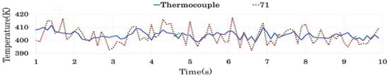
Figure 9. Comparison of T_Thc and T_Rec for 71 cycles.

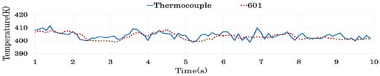
Figure 10. Comparison of T_Thc and T_Rec for 601 cycles.

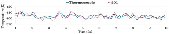
Figure 11. Comparison of T_Thc and T_Rec for 201 cycles.

Figure 12 shows the 2D reconstruction temperature distribution in 201 cycles in time from 1.0 to 9.0 s. The temperature of the peak area of the 2D distribution in each time was equal to that of the corresponding time at the 201 cycle reconstruction temperature in Figure 11. As illustrated in Figure 12, it can be seen that the maximum temperature was continuously distributed in the central area. For example, Figure 12b,h show a reconstruction temperature of approximately 410 K and 408 K in the central area, and Figure 10 shows also the same temperature at that time. This was the same in other times.

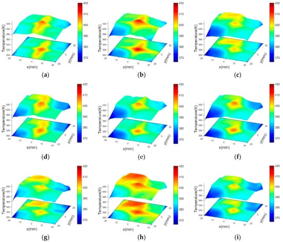
Figure 12. 2D reconstruction temperature distributions at 201 cycles: (a) 1.0 s; (b) 2.0 s; (c) 3.0 s; (d) 4.0 s; (e) 5.0 s; (f) 6.0 s; (g) 7.0 s; (h) 8.0 s; and (i) 9.0 s.

This study presented the statistical analysis procedure and the appropriate cycle to improve TDLAT performance when measuring time series-based 2D temperature in idle mode of engine. To the best of our knowledge, this is the first attempt to present the criteria for cycle selection through the similarity analysis when based on signal stabilization technique. This signal stabilization technique was more effective in error reduction than the conventional polynomial reduction method when converting signals into absorption spectra.

However, limitations of this study include (i) it was only tested in idle mode of a particular engine, so additional experiments are required in operation mode with relatively large temperature variations; and (ii) in idle mode, the temperature variation in the peak area was uniformly measured only for that area, but it is also necessary to check the need for measurements in other areas.

To overcome these limitations, the following studies will be carried out in the future: (i) conduct a time series-based 2D temperature measurement study by applying the latest statistical techniques (i.e., linear Bayesian absorbance inference, Tikhonov regularization, and so on) to provide a fast and accurate case of reconstruction temperature calculation and (ii) typically, the reconstruction temperature is verified by TC measurements. The reliability of verification will depend on the TC measurement method, therefore studies on the TC verification methodology will also be conducted; and (iii) the size of the laser grid will affect the bias of reconstruction temperature. We would like to conduct a study on the selection of optimal grid sizes to minimize bias.

References

- Amin, R.; Galen, B.F.; John, W.H.; Joseph, R.T.; James, D.P.; Christine, K.L. Rapidly pulsed reductants for diesel NOx reduction with lean NOx traps: Effects of pulsing parameters on performance. Appl. Catal. B Environ. 2018, 223, 177–191. [Google Scholar]
- Perng, C.C.; Easterling, V.G.; Harold, M.P. Fast lean-rich cycling for enhanced NOx conversion on storage and reduction catalysts. Catal. Today 2014, 231, 125–134. [Google Scholar] [CrossRef]
- Lietti, L.; Artioli, N.; Righini, L.; Castoldi, L.; Forzatti, P. Pathways for N2 and N2O formation during the reduction of NOx over Pt–Ba/Al2O3 LNT catalysts investigated by labeling isotopic experiments. Ind. Eng. Chem. Res. 2012, 51, 7597–7605. [Google Scholar] [CrossRef]
- Roy, S.; Gord, J.R.; Patnaik, A.K. Recent advances incoherent anti-Stokes Raman scattering spectroscopy: Fundamental developments and applications in reacting flows. Prog. Energy Combust. Sci. 2010, 36, 280–306. [Google Scholar] [CrossRef]
- Steuwe, C.; Kaminski, C.F.; Baumberg, J.J.; Mahajan, S. Surface enhanced coherent anti-Stokes Raman scattering on nanostructured gold surfaces. Nano Lett. 2011, 11, 5339–5343. [Google Scholar] [CrossRef] [PubMed]
- Williams, B.; Edwards, M.; Stone, R.; Williams, J.; Ewart, P. High precision in-cylinder gas thermometry using laser induced gratings: Quantitative measurement of evaporative cooling with gasoline/alcohol blends in a GDI optical engine. Combust. Flame 2014, 161, 270–279. [Google Scholar] [CrossRef]
- Hoffman, D.; Münch, K.U.; Leipertz, A. Two-dimensional temperature determination in sooting flames by filtered Rayleigh scattering. Opt. Lett. 1996, 21, 525–527. [Google Scholar] [CrossRef]
- Itani, L.; Bruneaux, G.; Lella, A.; Schulz, C. Two-tracer LIF imaging of preferential evaporation of multi-component gasoline fuel sprays under engine conditions. Proc. Combust. Inst. 2015, 35, 2915–2922. [Google Scholar] [CrossRef]
- Cho, K.Y.; Satija, A.; Pourpoint, T.L.; Son, S.F.; Lucht, R.P. High-repetition-rate three-dimensional OH imaging using scanned planar laser-induced fluorescence system for multiphase combustion. Appl. Opt. 2014, 53, 316–326. [Google Scholar] [CrossRef]
- Deguchi, Y.; Yasui, D.; Adachi, A. Development of 2D temperature and concentration measurement method using tunable diode laser absorption spectroscopy. J. Mech. Eng. Autom. 2012, 2, 543–549. [Google Scholar]
- Ma, L.; Li, X.; Sanders, S.T.; Caswell, A.W.; Roy, S.; Plemmons, D.H.; Gord, J.R. 50-kHz-rate 2D imaging of temperature and H2O concentration at the exhaust plane of a J85 engine using hyperspectral tomography. Opt. Express 2013, 21, 1152–1162. [Google Scholar] [CrossRef] [PubMed]
- Busa, K.M.; Ellison, E.N.; McGovern, B.J.; McDaniel, J.C.; Diskin, G.S.; DePiro, M.J.; Capriotti, D.P.; Gaffney, R.L. Measurements on NASA Langley Durable Combustor Rig by TDLAT: Preliminary Results. In Proceedings of the 51st AIAA Aerospace Sciences Meeting Including New Horizons Forum and Aerospace Exposition, Grapevine, TX, USA, 7–10 January 2013. [Google Scholar]
- Busa, K.M.; Rice, B.E.; McDaniel, J.C.; Goyne, C.P.; Rockwell, R.D.; Fulton, J.A.; Edwards, J.R.; Diskin, G.S. Scramjet combustion efficiency measurement via tomographic absorption spectroscopy and particle image velocimetry. AIAA J. 2016, 54, 2463–2471. [Google Scholar] [CrossRef]
- Sun, P.; Zhang, Z.; Li, Z.; Gou, Q.; Dong, F. Study of two dimensional tomography reconstruction of temperature and gas concentration in combustion field using TDLAS. Appl. Sci. 2017, 7, 990. [Google Scholar] [CrossRef]
- Zhang, Z.R.; Pang, T.; Yang, Y.; Xia, H.; Cui, X.; Sun, P.; Wu, B.; Wang, Y.; Sigrist, M.W.; Dong, F. Development of a tunable diode laser absorption sensor for online monitoring of industrial gas total emissions based on optical scintillation cross-correlation technique. Opt. Express 2016, 24, 943–955. [Google Scholar] [CrossRef] [PubMed]
- Dickheuer, S.; Marchuk, O.; Tsankov, T.V.; Luggenhölscher, D.; Czarnetzki, W.; Ertmer, S.; Kreter, A. Measurement of the magnetic field in a linear magnetized plasma by tunable diode laser absorption spectroscopy. Atoms 2019, 7, 48. [Google Scholar] [CrossRef]
- Stritzke, F.; Kely, S.V.D.; Feiling, A.; Dreizler, A.; Wagner, S. TDLAS-based NH3 mole fraction measurement for exhaust diagnostics during selective catalytic reduction using a fiber-coupled 2.2-µm DFB diode laser. Opt. Express 2015, 119, 143–152. [Google Scholar] [CrossRef]
- Bolshov, M.A.; Kuritsyn, Y.A.; Romanovskii, Y.V. Tunable diode laser spectroscopy as a technique for combustion diagnostics. Spectrochim. Acta Part B 2015, 106, 45–66. [Google Scholar] [CrossRef]
- Xu, L.; Liu, C.; Jing, W.; Cao, Z.; Xue, X.; Lin, Y. Tunable diode laser absorption spectroscopy-based tomography system for on-line monitoring of two-dimensional distributions of temperature and H2O mole fraction. Rev. Sci. Instrum. 2016, 87, 013101. [Google Scholar] [CrossRef]
- Gamache, R.R.; Kennedy, S.; Hawkins, R.; Rothman, L.S. Total internal partition sums for molecules in the terrestrial atmosphere. J. Mol. Struct. 2000, 517–518, 407–425. [Google Scholar] [CrossRef]
- Rothman, L.S.; Gordon, I.E.; Barbe, A.; Benner, D.C.; Bernath, P.F.; Birk, M.; Bizzocchi, L.; Boudon, V.; Brown, L.R.; Campargue, A.; et al. The HITRAN2012 molecular spectroscopic database. J. Quant. Spectrosc. Radiat. Transf. 2013, 130, 4–50. [Google Scholar] [CrossRef]
- Hong, D.H.; Wang, L.; Truong, T.K. Low-complexity direct computation algorithm for cubic-spline interpolation scheme. J. Vis. Commun. Image Represent. 2018, 50, 159–166. [Google Scholar] [CrossRef]
- Deguchi, Y.; Noda, M.; Abe, M.; Abe, M. Improvement of combustion control through real-time measurement of O2 and CO concentrations in incinerators using diode laser absorption spectroscopy. Proc. Combust. Inst. 2002, 29, 147–153. [Google Scholar] [CrossRef]
- Choi, D.W.; Jeon, M.G.; Cho, G.R.; Kamimoto, T.; Deguchi, Y.; Doh, D.H. Performance improvements in temperature reconstructions of 2-D tunable diode laser absorption spectroscopy (TDLAS). J. Therm. Sci. 2016, 25, 84–89. [Google Scholar] [CrossRef]
- Zaatar, Y.; Bechara, J.; Khoury, A.; Zaouk, D.; Charles, J.-P. Diode laser sensor for process control and environmental monitoring. Appl. Energy 2000, 65, 107–113. [Google Scholar] [CrossRef]
- Doh, D.H.; Lee, C.J.; Cho, G.R.; Moon, K.R. Performances of Volume-PTV and Tomo-PIV. Open J. Fluid Dyn. 2012, 2, 368–374. [Google Scholar] [CrossRef]
- Choi, K.M.; Lee, J.T.; Jeon, S.G.; Hong, T.G.; Paek, J.K.; Han, S.H.; Yim, D.S. A review of fundamentals of statistical concepts in clinical trials. J. Korean Soc. Clin. Pharmacol. Ther. 2012, 20, 109–124. [Google Scholar] [CrossRef][Green Version]
- Cort, J.W.; Kenhi, M. Advantages of the mean absolute error (MAE) over the root mean square error (RMSE) in assessing average model performance. Clim. Res. 2015, 30, 79–82. [Google Scholar]
- Seo, M.K.; Yun, W.Y. Clustering based hot strip roughing mill diagnosis using Mahalanobis distance. J. Korean Inst. Ind. Eng. 2017, 43, 298–307. [Google Scholar]
- Wikipedia. Available online: https://en.wikipedia.org/wiki/Mahalanobis_distance (accessed on 23 September 2019).
- Yu, J.W.; Jang, J.Y.; Yoo, J.Y.; Kim, S.S. Fault detection method for steam boiler tube using Mahalanobis distance. J. Korean Inst. Intell. Syst. 2016, 26, 246–252. [Google Scholar] [CrossRef][Green Version]
- Minitab 19 Support. Available online: https://support.minitab.com/en-us/minitab/18/Assistant_Two_Sample_t.pdf (accessed on 20 November 2019).
© 2019 by the authors. Licensee MDPI, Basel, Switzerland. This article is an open access article distributed under the terms and conditions of the Creative Commons Attribution (CC BY) license (http://creativecommons.org/licenses/by/4.0/).