Featured Application
A new photovoltaic inverter weighted efficiency formulation to be used in the equatorial region as part of energy yield estimation for a solar photovoltaic system installation’s return of investment.
Abstract
Photovoltaic inverter conversion efficiency is closely related to the energy yield of a photovoltaic system. Usually, the peak efficiency (ηmax) value from the inverter data sheet is used, but it is inaccurate because the inverter rarely operates at the peak power. The weighted efficiency is a preferable alternative as it inherently considers the power conversion characteristics of the inverter when subjected to varying irradiance. However, since the weighted efficiency is influenced by irradiance, its value may not be appropriate for different climatic conditions. Based on this premise, this work investigates the non-suitability of the European weighted efficiency (ηEURO) for inverters installed in the Equatorial region. It utilizes a one year data from the Equatorial irradiance profile to recalculate the value of ηEURO (ηEURO_recal) and to compare it with the original ηEURO. Furthermore, a new weighted efficiency formula for the Equatorial climate (ηEQUA) is proposed. Validation results showed that calculated energy yield with ηEQUA closely matched the real energy yield of 3 kW system with only 0.16% difference. It is envisaged that the usage of ηEQUA instead of ηmax or ηEURO will results in a more accurate energy yield and return of investment calculations for PV systems installed in Equatorial regions.
1. Introduction
Prior to installation, the photovoltaic (PV) system provider (PVSP) performs a site survey to determine the suitability of the location and to propose the most appropriate system design. Then, the energy yield (Esys) prediction report will be provided to the customer. This report allows for the return of investment (ROI) or the payback period to be calculated and correspondingly, the financial capital can be secured [1]. One important element in the Esys calculation is PV inverter conversion efficiency. For convenience, many PVSP use the maximum (peak) efficiency (ηmax) value from the inverter datasheet to compute Esys [2,3]. However, it has to be noted that the ηmax refers to the maximum achievable conversion efficiency of the dc-ac power converter (or inverter) under the standard test condition (STC) (STCs: Irradiance: 1000 W/m2, Temperature: 25 °C, Air Mass: 1.5 AM). In practice, the PV system rarely operates at STC. For example, in a region that experiences the Equatorial climate, the STC condition is achievable only for a limited period of the day. At most times, the system is subjected to a much lower irradiance (G). Moreover, the operating (module) temperature (T) is typically in excess of 35 °C throughout the day [4].
Alternatively, the weighted efficiency—such as the European (ηEURO) and the California Energy Commission (ηCEC) can be used for Esys computation. The weighted efficiency is based on the consideration that, on average (time per year), the inverter does not operate at STC. Instead, it is subjected to the continuous variation of irradiance and temperature. Since the power loss of the power (semiconductor) switches inside the inverter is dependent on the current level at which they operate, the efficiency value is “adjusted” in order to accommodate for the variation in the operating condition. Furthermore, the efficiency of the inverter is affected by the fixed losses and ohmic losses. The former is normally due to the power consumption of the controller and driver circuits, while the latter is related to the other resistive (I2R) losses. Thus, the weighted efficiency is considered to be more representative of the real inverter performance. Despite this advantage, it is obvious that the weighted efficiency is specific to a particular climatic region; therefore, its usage in different meteorological conditions can lead to inaccurate Esys prediction. For example, an inverter that operates in Europe will not give the same output if it were to be installed in the Equatorial region because the irradiance profiles between the two are markedly different [5]. Correspondingly, if the same value of ηEURO is used, the Esys, the ROI and payback period for the latter will be wrongly calculated.
Notwithstanding this clear mismatch, it is rather surprising to discover that no work has been undertaken to determine the suitability of ηEURO for inverters installed in an Equatorial climate. To date, most PVSP still consider ηmax or ηEURO as the benchmark for efficiency, despite the significant difference in the irradiance and temperature profiles. Perhaps, during the initial growth of the PV industry, the market share of the countries outside Europe was much lower, so providing a separate weighed efficiency number for the inverter was not urgent. However, with the recent rapid growth of PV installations in the Equatorial region, there is a need to have a more accurate prediction of Esys. Thus, it is timely to carry out an investigation on this matter.
This work is carried out with two primary objectives. First is to prove the hypothesis that if a PV system is installed in the Equatorial region, the usage of ηEURO from the datasheet will not be accurate. In other words, the ηEURO needs to be recalculated to reflect the inverter performance under the influence of the Equatorial irradiance profile. Second, once this fact is established, a new formula for weighted efficiency that is suitable for the Equatorial region is to be formulated. To achieve these goals, the first step is to gather a one year in-plane irradiance (G) dataset from a dedicated weather station. As required by the international standards and test protocol [6,7,8], the G data are used as an input to the PV array simulator (PVAS), which then feed the inverter under test. The output of the PVAS is connected the ac grid, while the input dc power (Pdc) and the output ac power (Pac) are measured at a specific level of operation. From these data, the efficiency of the ηEURO for the inverter is re-calculated and compared with the value given by the data sheet. Using the same data set, the formula for efficiency for equatorial climate (ηEQUA) is derived. To validate the correctness of ηEQUA, the power data from a 3 kW real system are used.
2. Review of PV Inverter Efficiency
2.1. Overview
Apart from the module, the inverter is the next most crucial and costly component in a PV system. Since the life-cycle of the system is long, i.e., well over 20 years, the effective influence of inverter efficiency has to be factored into the overall system performance. Based on references [2,3], the energy yield, Esys can be predicted using
In (1), Parray refers to the rated power of the module, PSH is the peak sun hour of irradiation, ftemp is the losses due to temperature, fmm is the manufacturer’s tolerance or mismatch, fdirt is the loss which is due to the accumulation of dirt on the panel surface, and ηcable is the efficiency of the DC cable that is used to connect the PV panel and the DC side of the inverter. The last term in the equation, i.e., ηinv refers to the inverter efficiency. As a rule of thumb, an inverter which is 1% less efficient is quoted to be 10% comparatively cheaper [9].
Figure 1 depicts the tree diagram of PV inverter efficiency classification. It has two components: the conversion (ηinv) and the maximum power point tracking (MPPT) efficiency (ηMPPT). The ηinv is simply the ratio of the output (ac) power to input (dc) power, and is directly related to the efficiency of converter hardware. On the other hand, the ηMPPT reflects the ability of the MPPT algorithm to tracks the maximum point on the P-V characteristic curve at any instant. It is the ratio of the actual power that is extracted from the module to the maximum theoretical power that can be achieved from the P-V curve. The ηMPPT influences the power converter by adjusting its duty cycle so that it always operate at the maximum point for a given temperature and irradiance level. The total efficiency is defined as the multiplication of ηinv and ηMPPT [10]. This work concentrates on the ηinv, as the MPPT efficiency has already been extensively covered elsewhere [11].
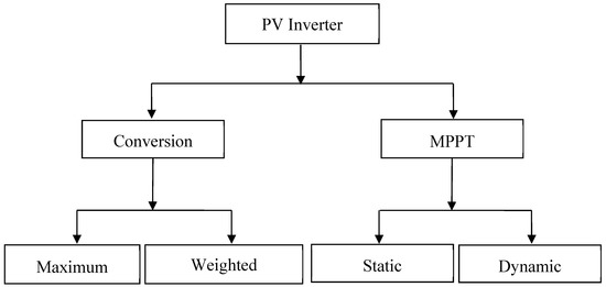
Figure 1.
Tree diagram of PV inverter efficiency [11].
To simplify the calculation for Esys, many PVSPs assume ηinv equals ηmax [2]. The ηmax, which is usually given in the datasheet, indicates the maximum reachable efficiency achieved by the inverter, measured using the STC. Typically, the peak power is achieved when the inverter operates at approximately 70%–80% of its rated power. However, the irradiance does not necessary falls into the range where the inverter is at its peak performance. Moreover, the usage of ηmax is not realistic because the inverter seldom operates at STC during the field operation. Consequently, the application of ηmax results in an over-rated Esys value, causing inaccurate prediction of the ROI and the payback period. The weighted efficiency, on the other hand, takes into account the performance of the inverter when subjected to varying irradiance profile. Since the irradiance is directly related to the input power of the inverter, the conversion efficiency varies according to power level at which the inverter operates. Thus, the weighted efficiency is more representative of the inverter performance because it matches the operational condition with the power converter characteristics.
2.2. Formulation of Weighted Efficiency
The general approach to derive the weighted efficiency can be found in several documents, particularly the IEC 61683 and the EN 50530 Standard [6,7,8]. These standards recommended that the weighted efficiency equation to be developed in a controlled laboratory environment using the PV array simulator. The output of the simulator emulates the output of a real PV panels, which is connected to the inverter being tested. The simulator is fed by a one-year G profile that is averaged as a one-day dataset. To compute the efficiency, the input and output power data (i.e., the Pac and Pdc) of the inverter need to be recorded. Another important feature is that the weighted efficiency is computed with the assumption that the back panel temperature (T) is kept constant at 25 °C. Only G is made variable so that the performance of the inverter can be made comparable when tested in a different climate.
In principle, the idea of weighted efficiency is based on the irradiance-duration (G vs. time) curve. An example of such curve is shown in Figure 2. In this case, the inverter operates at four levels of operation. The level of operation is related to Pdc/Pdc_rated, where Pdc is the dc input power to the inverter (which is proportional to G), while Pdc_rated is the rated dc power of the inverter (given by the data sheet). The choice for the number of level of operation is arbitrary. Any number can be used as long as the Pac, Pdc, and G data are available. However, to simplify the efficiency formula, Pdc/Pdc_rated are grouped into several ranges.
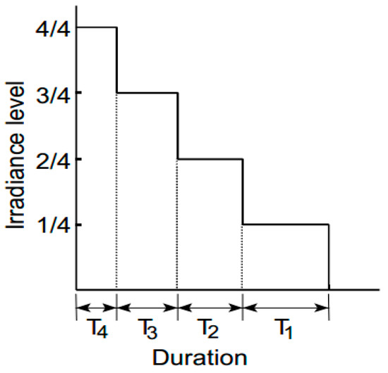
Figure 2.
Example of irradiance-duration curve with four levels of operation [6,7,8].
The formula for the weighted efficiency, (ηWT) is calculated as the sum of the product efficiency (at each level of operation) and its corresponding weightage, as given by (2). The weightage refers to the amount of time (Tn) that the inverter operates (at a specific level of operation) divided by the sum of irradiance level for the whole duration of the inverter operating time (TWT), i.e., Tn/TWT. The efficiency is simply the ratio of the output (Pac) to input (Pdc) power at a specific level of operation.
For the irradiance-duration curve shown in Figure 2,
where
- ηWT = weighted efficiency
- TWT = 1T1 + 2T2 + 3T3 + 4T4
- η1/4 = is the efficiency value when Pdc is 1/4 of Pdc_rated
2.3. Types of Inverter Weighted Efficiency
Currently, the most widely used weighted efficiency is the ηEURO. Its formulation is based on an hourly irradiance dataset gathered from a town called Trier, Germany [12,13]. In general, ηEURO represents the inverter installed in regions that receive moderate irradiance penetration [14,15]. Its formula is given as
Since ηEURO was developed before the existence of IEC 61724 and IEC 61683 Standards, it does not conform to the maximum of a 15 min sampling interval requirement. Instead, it was based on hourly irradiance sampling, which was manually recorded every three hours [12,13]. Recently, several researchers revisited the computation of ηEURO using one second sampling time. However, the difference in the outcome was only 0.2% and thus, the finding is not considered to be significant [13]. The ηEURO formula is characterized by six pre-determined levels of operation: i.e., 5%, 10%, 20%, 30%, 50%, and 100%. The ranges for Pdc/Pdc_rated that form the level of operation is shown in Table 1. For each level, a group of Pdc/Pdc_rated is assigned; for instance, level 20% comprises of Pdc/Pdc_rated that fall between 15% and 25%. Furthermore, the associated weightages are also shown. The heaviest weightage of 0.48 occurs at level of operation that equals 50%. This means that for nearly half of the operational time (T/TW), the inverter is operating at approximately 50% of its rated power. On the other extreme, the lowest weightage is 0.03, which occurs when level of operation equals 5%. This implies that for 3% of the operational time, the inverter operates at approximately 5% of its capacity. In the case of ηEURO, it is unclear how the weightage is determined. This most likely occurs is through trial and error.

Table 1.
The ranges for Pdc/Pdc_rated and weightage for each level of operation for ηEURO.
The California Energy Commission weighted efficiency (ηCEC) is based on one second sampling of the irradiance data, collected from Sacramento, California [16]. It has become a popular indicator to quantify the performance of the inverter in a region with high irradiance [13]. Similar to ηEURO, it also has six levels of operation. However, the efficiency at each level of operation assumes a different value. Furthermore the weightage differ as follows:
By comparing (4) and (5), it can be observed that the ηCEC is more balanced in terms of the range of efficiency distribution that the inverter operates in. In contrast, the ηEURO pays more attention towards the range under 50% of PV inverter efficiency.
Besides ηCEC and ηEURO, there were other attempts to formulate the weighted efficiency according to respective local climates. The Izmir Efficiency (ηIZM) is based on a one minute sampling of irradiance data of Izmir, Turkey [17]. The formulation of ηIZM is done using the PV array simulator at the Austrian Institute of Technology (AIT), Vienna. The resulting equation, i.e., (6), resembles the simplified version of ηCEC, but with the omission of weightages at levels of operation equal to 20% and 100%. Moreover, the power level efficiency at 75% was changed to 70%. These similarities are no coincidence. If the world map of Koppen-Geiger Climatic Classification System (KGCCS) shown in Figure 3 is referred to, Izmir and Sacramento (where the data for ηCEC is collected) actually share the same climatic condition. It is labeled as “Csa”, which is characterized by a mild temperate climate as well as a dry and hot summer [18].
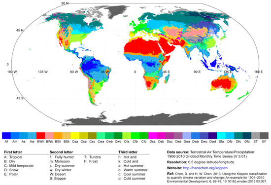
Figure 3.
World map of the Koppen-Geiger climate classification system [18].
The first localized weighted inverter efficiency from India is the Chennai Efficiency (ηCHE) [19]. Chennai is a city located in the Southeast of India. Under the KGCCS, the climate is marked as “Aw: tropical, with dry winter”. The ηCHE was based on the data gathered in 2010–2013 of a working 155 kW PV system. However, these procedures did not comply with the IEC 61683 [6,7,8], in which the efficiency must be derived using the PV array simulator that is fed by the local irradiance profile at a fixed temperature of 25 °C. In this case, both of the irradiance and temperature varies. Furthermore, the irradiance was measured horizontally (not in-plane), which did not comply with IEC 61724 [20,21]. The developed equation for ηCHE is
Another Indian weighted efficiency is the Kanpur Efficiency (ηKAN) [22]. As the name suggests, the ηKAN is derived using the irradiance collected at the Indian Institute of Technology, Kanpur, in Northern India. Under the KGCCS, the climate is marked as “Cwa: mild temperate, with a dry winter and hot summer”. Unfortunately, as with the case of the Chennai efficiency, the ηKAN is not derived using the PV simulator as required by IEC 61683. As a replacement, the real data of a 40 kW PV system is used. Moreover, it is not based on a yearly data as suggested by reference [20] and reference [21]. Instead the irradiance data is a sample of two sunny days (23 January 2014 and 17 February 2014) is used. Hence, it is not surprising that one of the significant features of ηKAN is the large weightage (0.84) given for level of operation of 100% (0.84), i.e.,
In conclusion, it can be deduced that of among existing weighted efficiencies, only the ηCEC and ηIZM were formed according to the required standards [6,7,8,20,21]. However, the ηIZM can be deemed as being redundant since both ηIZM and ηCEC actually represent the same climatic profile. Even though this profile is shared by many countries situated in the Mediterranean, the ηCEC is not popular, except in North America. Despite the inadequacies of ηEURO (with regards to the compliance of standards) it is still the most common standard in the rest of the world. This is mainly due to similarities in the voltage and frequency settings, which favor the ηEURO. Furthermore, ηEURO was introduced much earlier than other weighted efficiency formula, and has remained as the standard bearer ever since.
3. Methods
As shown in the KGCCS map, the Equatorial climate, i.e., “Af: tropical, fully humid” is shared by more than 20 countries across three continents. This climate is characterized by a relatively constant temperature, high precipitation (rain), and high cloud presence throughout the year [23]. Furthermore, there is no clear trend of four distinct seasons, as is commonly experienced by temperate countries. It is therefore reasonable to assume that the true performance of PV inverters operating in temperate countries can be different from others installed outside them. Based on this hypothesis, the first objective of this work is to prove that ηEURO is unsuitable for inverters installed in the Equatorial climate. Once this fact is established, the second objective is formulated, namely a new weighted efficiency formula for the Equatorial climate. To achieve these objectives, the following activities are carried out: (1) collecting one year (Equatorial climate) irradiance data from weather stations, (2) running an inverter with a PV array simulator using the collected data, (3) measuring the input and output power, (4) re-calculating the ηEURO of the inverter, (5) formulating the weighted efficiency formula for the Equatorial climate (ηEQUA), and (6) validating ηEQUA using data from a practical PV system. For convenience, this methodology is summarized as a flowchart shown in Figure 4.
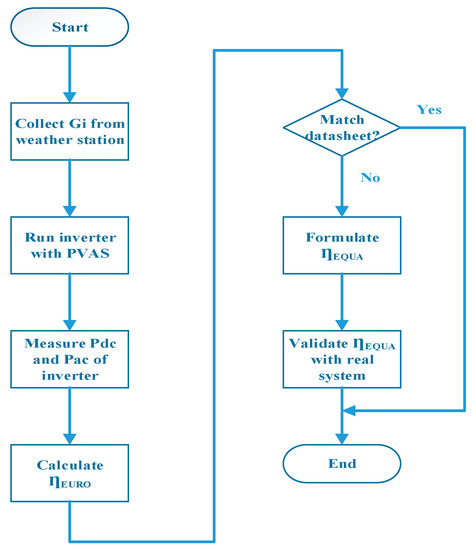
Figure 4.
Flowchart of the methodology.
3.1. The Weather Station
The meteorological data of interest data are collected from a dedicated weather station located at the Universiti Teknikal Malaysia Melaka, Malaysia (GPS coordinate of 2°12′0″ N, 102°15′0″ E) [4,24]. The photographs of the set-up are shown in Figure 5. The location can be considered as a typical reference for the Equatorial region. The collected data are the horizontal or global irradiance (Gh), tilted (in-plane) irradiance (Gi), ambient temperature (Ta), and module temperature (Tm). To measure Gh and Gi, two CMP11 secondary standard pyranometers are used. Furthermore, the HMP 155 ambient temperature sensor and the fast response thermocouple type E are utilized to measure Ta and Tm, respectively. The specifications of the measurement devices and sensors are in compliance to the IEC 61724 [20]. These sensors are connected to the electronic data acquisition system. The data are sampled, logged at every one second interval, and stored in a dedicated server. The latter is equipped with a redundant array of independent disks (RAID) system to preserve the continuity of the saved data in the case of hard disk drive failure. From the one second base sampling, the data is processed (averaged) to obtain the 1 min, 5 min, hourly, daily, and monthly data size. For the purpose of producing a weighted efficiency equation, only the tilted irradiance profile is needed. The temperature information is not used because the weighted efficiency formulation PV array simulator requires the module temperature to be fixed, i.e., st 25 °C.

Figure 5.
The photographs of hardware used in data collection: (a) the CMP11 pyranometer; (b) data acquisition for weather sensors.
Figure 6 shows the in-plane irradiance (Gi) profile, logged by the weather station on 9 April 2014 [4]. The data is sampled in one second. The profile characterizes a typical day of Equatorial weather: clear sky early in the morning until midday before shifting to a cloudy sky later in the day. However, to produce a one year daily average, a one minute average sampling time is suggested by the IEC 61724 [20], as well as by the Australian PV System Monitoring Guideline (2013) [21]. Based on these recommendations, the one second sampled data (taken from 1 January 2014 to 31 December 2014) is averaged to one minute. In this paper this dataset is known as the “Equatorial data”.
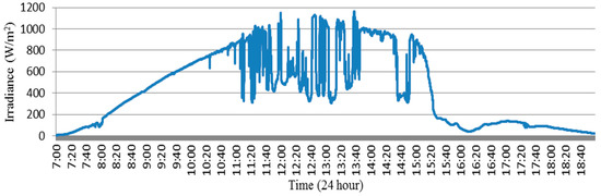
Figure 6.
Example of one second sampled in-plane irradiance daily data in 2014 [4].
3.2. The PV Array Simulator
In order to have consistent formulation of inverter efficiency, the measurements must be conducted in a laboratory environment, where the irradiance and temperature can be controlled reliably. It is difficult to achieve these conditions using the physical PV array (in the field) due to the meteorological uncertainties (particularly temperature variation). Thus, the PV array simulator (PVAS) from Austrian Institute of Technology (AIT) was used to emulate the PV modules of specific types [9,24]. Unlike the normal simulator (which is switched mode power supply), the PVAS is built using a linear high-voltage Metal Oxide Semiconductor Field Effect Transistor (MOSFET). As a result, the effect of switching frequency ripple on the dc output is minimized. The measured irradiance data (Gi from the weather station) was used as an input to the PVAS. Using these values, a unique I-V characteristic curve was generated. Then using a script generator, a continuous profile of output power (based on the I-V curve) was produced at the output of the PVAS. Note that to compute the weighted efficiency, the temperature was set to be constant at 25 °C.
Figure 7 depicts the overall block diagram used to measure the efficiency of the inverter, while Figure 8 shows the photograph of the actual laboratory test set-up. The Gi data from the weather station was converted into a specific format that is readable using the PVAS. Since the data is obtained from crystalline modules, the same technology was set in the PVAS parameters setting. Furthermore, the critical inverter specifications, i.e., Voc, Isc, Vmpp, and Impp were also specified [7]. The output of the PVAS was connected to the tested inverter and the latter was tied to the grid. To avoid measurement uncertainties (due to the voltage and frequency fluctuation), the grid was emulated using an ac power source, connected to a resistive load. The ratio between the module power and the dc side power of the inverter was set to 1:1. This ratio is recommended by references [25,26]. The electrical properties of the inverter, namely the input dc (VDC, IDC) and output ac (Vac and Iac), were logged using a PM 6000 power analyzer. From these quantities, the Pdc and Pac were computed, respectively. Four inverters with different technologies and ratings were tested. Their specifications are described in Table 2.
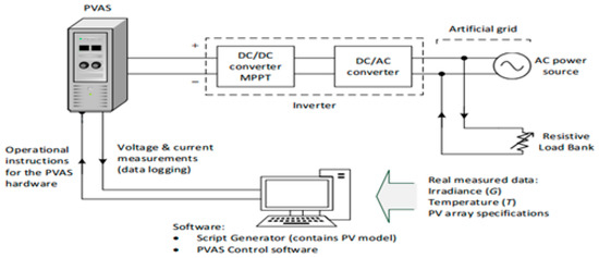
Figure 7.
Block diagram of the PV inverter test.
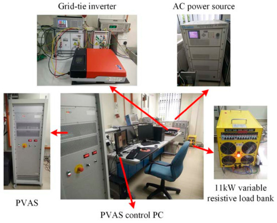
Figure 8.
Actual PV inverter test set-up.
Table 2.
The electrical properties of the tested PV inverters.
4. Discussion
4.1. Recalculated Euro Efficiency from Measured Equatorial Data
To determine whether ηEURO is suitable for an inverter installed in the Equatorial region, its value was recalculated using the irradiance profile of the region. The one year irradiance profile from the weather station was loaded into the PVAS and the output was used to drive the inverter. The module temperature (Tm) was held constant at 25 °C. By measuring the output power (Pac) and input power (Pdc), the efficiency of the inverter (ηmeas) was obtained. For the SB3000HF inverter, since the number of logged data that it produced was 593 (this is not necessarily the same for all inverters), the number of Pdc/Pdc_rated values and level of operation are the same. Correspondingly,
To emulate the original ηEURO equation, the Pdc/Pdc_rated values were grouped into six levels of operation. Thus, the 593 logged data were grouped into six ranges [13]. Taking the SB3000HF inverter as an example, these boundaries for the Pdc/Pdc_rated are summarized in Table 2. The six level of operation were 5%, 10%, 20%, 30%, 50%, and 100%. Note that, the 5% level has Pdc/Pdc_rated ranged from 0 to 7.5%; the 10% level has a Pdc/Pdc_rated ranged from 7.5 to 15% and so on. These ranges were adopted to be consistent with the original ηEURO formula. Similarly, the weightage for each corresponding level was adopted from the ηEURO. They were 0.03, 0.06, 0.13, 0.10, 0.48, and 0.20, respectively. Furthermore, for every level of operation, an average conversion efficiency (ηmeas_ave) was computed. It was the average measured efficiency of each logged data in that particular range. The weighted efficiency was the sum of multiplication of the ηmeas_ave and weightage, as shown in Table 3. Hence, the general form of weighted efficiency for the six level of operation can be written as
Table 3.
The ηEURO_recal values for the four different inverters (G = Gi and Tm = 25 °C).
The ηEURO_recal was the recalculated ηEURO when the inverter was operated under the Equatorial condition. Since the (same) ηEURO weightage was used for ηEURO_recal computation, a certain amount of difference to the former was expected. From Table 4, it can be seen that the ηEURO_recal was lower (between 0.27% and 2.06%), depending on the inverter technology and size. This observation suggests that if an inverter with a ηEURO datasheet was operated in the Equatorial climate, its energy yield would be lower than the computed value (using ηEURO). The difference was inevitable because the weightage remains constant, while the irradiance profile has changed significantly. Thus, it was proven that usage of a ηEURO Equatorial climate is unsuitable and there is a need to derive a new weighted efficiency that reflects the meteorological condition of this region.
Table 4.
Differences between ηEURO from the datasheet and ηEURO_recal.
4.2. Methodology for Determination of Equatorial Efficiency
It is clear that to determine a correct value of weighted efficiency for the Equatorial region, it is necessary to modify the weightage for each level of operation. If the original value of weightage (from ηEURO) is used, it will result in a different value. This is shown by the discrepancies between ηEURO and ηEURO_recal in Table 4. Thus, to formulate the Equatorial efficiency (ηEQUA), a new set of weightage needed to be determined. However, to maintain consistency with ηEURO, six levels of operation with similar Pdc/Pdc_rated range (as shown in Table 1) were used.
Recall that the weightage is Tn/TWT, where Tn is the duration at which the inverter operates at a certain irradiance level and TWT is the entire duration of the inverter operating time. Figure 9 illustrates the irradiance-duration curve produced by the SB3000HF inverter constructed from the one year Equatorial irradiance data from the weather station [6,7,8]. Based on the gathered data, the Pdc/Pdc_rated values were grouped into six level of operations. The duration for each level is denoted by T1, T2, …, T6. For example, for T5 the level of operation is 50%. The amount of time in which the inverter operates in this condition (over the entire duration) is 43%. Thus, the weightage for this level is 0.43. Similar evaluations can be made for other levels of operation: the weightage for every level of operation can be written as 0.9, 0.8, 0.9, 0.13, 0.43, and 0.18.
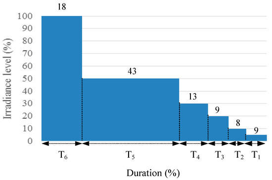
Figure 9.
The irradiance-duration curve produced by the SB3000HF inverter.
The other important variables of the weighted efficiency are the Pac and Pdc measurements. They have to be measured at every value of Pdc/Pdc_rated. For every level of operation, the Pdc/Pdc_rated was confined within a certain range, as shown in Table 5. Thus the efficiency calculations within this range have to be averaged—similar to the ones performed for ηEURO_recal. The summation of the multiplication between ηmeas_ave and weightage results in the weighted efficiency of the inverter. The final values of ηEQUA for SB3000HF, SB700LF, K4200TL, and K7900TL are shown in Table 5, Table 6, Table 7 and Table 8, respectively.
Table 5.
Weighted efficiency for the SB3000HF inverter when G = Gi and T = 25 °C with individual weightage.
Table 6.
Weighted efficiency for the SB700LF inverter when G = Gi and T = 25 °C with individual weightage.
Table 7.
Weighted efficiency for the K4200TL inverter when G = Gi and T = 25 °C with individual weightage.
Table 8.
Weighted efficiency for K7900TL inverter when G = Gi and T = 25 °C with individual weightage.
Since the analysis was conducted for four inverters (with different technology), a generalized relationship for ηEQUA needs to be determined. Because the weightage for each inverter shows very small variations compared to the other ones, it is sufficient to take a simple average of the individual weightage for every inverter at every level of operation. As shown in Table 9, the average weightage was 0.0875, 0.1125, 0.0800, 0.1250, 0.4400, and 0.1550, respectively. To simplify the formula, the numbers were rounded to two decimal places. Thus, the suggested Equatorial Efficiency (ηEQUA) formula can be written as
Table 9.
Determination of general ηEQUA weightage.
With the adoption of the new ηEQUA, Table 10 shows the summary of the difference in the weighted efficiency for the four inverters. As can be observed, in all cases, the ηEQUA is less than the ηEURO from the datasheet. The ηEQUA is also lower than the recalculated ηEURO, i.e., ηEURO_recal. The differences are in the range from 0.5% to 3.99%. These findings imply that if ηEURO is used to compute the Esys, it will lead to incorrectly high energy production estimation.
Table 10.
Differences between ηEURO from datasheet, recalculated ηEURO, and suggested ηEQUA.
4.3. Results Validation
It is difficult to validate the accuracy of the ηEQUA formula using the power data obtained from a real PV system. This is because in the Equatorial region, the temperature rarely remains at 25 °C throughout the day. Such a condition only occurs early in the morning when the irradiance is very low, i.e., less than 100 W/m2. However, during that time, the inverter is either in sleep mode or in grid synchronization mode. One practical approach is to validate the ηEQUA (which is formulated at 25 °C) by comparing the measured energy yield (Esys_meas) of a real system to the calculated energy yield (Esys_calc). The latter is calculated using
To determine Esys_calc, the number of days is set at 365, Parray at 3 kW, PSH is fixed according to the designated month or year, ftemp at 98%, fmm at 95%, fdirt at 97%, and ηcable at 98%. These made the accumulation of errors set at 0.8. These values are widely used and have been verified by reference [2]. While these variables remain fixed, the ηinv is varied using either the value ηmax, ηEURO or ηEQUA. This is to compare the computed energy yield when using three types of weighted efficiency formulas. By taking the absolute difference between Esys_meas and Esys_calc, i.e.,
The weighted efficiency which results in Esys_diff being the closest value to zero can be considered to be the most appropriate setting for the Equatorial region. The real PV system is a 3 kW roof-top grid-connected system with a 1:1 (PV module: inverter) sizing ratio. The array comprises of twelve 255 W monocrystalline modules, facing South at 10° tilt angle. The strings from the panels are connected to a SB3000HF inverter. As suggested in references [2,3], the Esys calculation is only valid when the data is logged for one year. Figure 10 shows the energy produced, logged throughout the year 2014. The total Esys_meas for the year is 4141.7 kWh. The computed values Esys_calc using ηmax, ηEURO, and ηEQUA are shown in Table 11. The Esys_diff are 99.10, 59.47, and 6.63 kWh, respectively. Clearly, the computation using ηEQUA results Esys_diff is nearest to zero. Thus, it can be concluded that ηEQUA is the best option to represent the inverter efficiency for the Equatorial region.
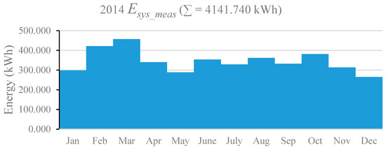
Figure 10.
Energy produced from a real 3 kW PV system in 2014.
Table 11.
Validation results of Esys with different types of PV inverter efficiencies.
5. Conclusions
In this paper, experimental work was done on four inverters with different sizes and technologies to investigate the suitability of the application of ηEURO in the Equatorial climate due to the overrated nature of ηmax. PVAS simulation results using a recalculated ηEURO of the four inverters under an Equatorial irradiance profile showed nonconformance to the ηEURO, as stated in each of the inverters’ datasheets. This is expected since that PV inverter’s weighted efficiency is influenced by irradiance and different climatic region will have its own irradiance profile. Hence, ηEQUA was developed to better represent the actual weighted efficiency of PV inverter in the equatorial region. This finding was further validated when its Esys_calc was compared with Esys_meas of a real grid-connected PV system. The comparison shows that Esys_calc with ηEQUA instead of ηEURO or ηmax matched the real system Esys_meas more closely. Thus, it is hoped that the use of ηEQUA instead of the current practice of ηmax in the Esys calculation will better indicate the expected output from a PV system installed and therefore will accurately specify the correct ROI period for the system owner.
Author Contributions
All authors contributed equally to this work. All authors have read and agreed to the published version of the manuscript.
Funding
This research was funded by Ministry of Higher Education Malaysia (MoH) through Fundamental Research Grant Scheme (FRGS) with ref. no. FRGS/1/2014/TK06/UTEM/03/2. It was also co-funded by the Malaysia Rising Star Award (MRSA) grant from the Ministry of Education Malaysia (MoE) and managed by the Research Management Center, Universiti Teknologi Malaysia, under the Vot No.130000.7823.4F919.
Acknowledgments
This paper is the output of the research collaboration between the Universiti Teknikal Malaysia Melaka (UTeM) and the Universiti Teknologi Malaysia (UTM).
Conflicts of Interest
The authors declare no conflict of interest.
References
- Kalogirou, S.A. Solar Economic Analysis. In Solar Energy Engineering, 2nd ed.; Elsevier Science Publishing Co Inc.: Waltham, MA, USA, 2014; pp. 701–734. [Google Scholar]
- Omar, A.M.; Shaari, S.; Sulaiman, S.I. Grid-Connected Photovoltaic Power Systems Design; Sustainable Energy Development Authority Malaysia (SEDA): Putrajaya, Malaysia, 2012; pp. 73–76. [Google Scholar]
- Clean Energy Council. Grid-Connected Solar PV Systems (No Battery Storage)-Design Guidelines for Accredited Installers; Clean Energy Council: Melbourne, Australia, 2012; Issue 6. [Google Scholar]
- Tropical Weather Station, Smart Grid Solar Photovoltaic (SGPV), Energy and Power Systems Group, Centre of Electrical, Robotics and Industrial Automation (CERIA), Universiti Teknikal Malaysia Melaka. Available online: http://ceria.utem.edu.my/lab-spsg-home.html (accessed on 1 January 2015).
- Fang, H.; Li, J.; Song, W. Sustainable site selection for photovoltaic power plant: An integrated approach based on prospect theory. Energy Convers. Manag. 2018, 175, 755–768. [Google Scholar] [CrossRef]
- IEC. IEC 61683: Photovoltaic Systems—Power Conditioners—Procedure for Measuring Efficiency; IEC: Geneva, Switzerland, 1999. [Google Scholar]
- CENELEC. EN 50530: Overall Efficiency of Grid-Connected Photovoltaiv Inverters; CENELEC: Brussels, Belgium, 2010. [Google Scholar]
- Bower, W.; Whitaker, C.; Erdman, W.; Behnke, M.; Fitzgerald, M. Performance Test Protocol for Evaluating Inverters Used in Grid-Connected Photovoltaic Systems. Sandia National Laboratory Technical Report. Available online: https://www.gosolarcalifornia.ca.gov/equipment/documents/2004-11-22_Test_Protocol.pdf (accessed on 24 December 2019).
- Bletterie, B.; Brundlinger, R.; Lauss, G. On the Characterisation of PV Inverter’s Efficiency—Introduction to the Concept of Achievable Efficiency. Prog. Photovolt. Res. Appl. 2011, 19, 423–435. [Google Scholar] [CrossRef]
- Haberlin, H.; Borgna, L.; Kaempfer, M.; Zwahlen, U. Total Efficiency Htot—A New Quantity for Better Characterization of Grid-connected PV Inverters. In Proceedings of the 20th European Photovoltaic Solar Energy Conference (EUPVSEC), Barcelona, Spain, 6–10 June 2005; pp. 1–4. [Google Scholar]
- Salam, Z.; Rahman, A.A. Efficiency for Photovoltaic Inverter: A Technological Review. In Proceedings of the IEEE Conference on Energy Conversion (CENCON), Johor Bahru, Malaysia, 13–14 October 2014; pp. 175–180. [Google Scholar]
- Hotopp, R. Private Photovoltaic-Stromerzeugung-Sanlagen im Netzparallelbetrieb, 2; Auflage, RWE Energie AG: Essen, Germany, 1991. [Google Scholar]
- Burger, B.; Schmidt, H.; Goeldi, B.; Bletterie, B.; Bruendlinger, R.; Haberlin, H.; Baumgartner, F.; Klein, G. Are We Benchmarking Inverters on the Basis of Outdated Definitions of the European and CEC Efficiency? In Proceedings of the European Photovoltaic Solar Energy Conference (EUPVSEC), Hamburg, Germany, 21–25 September 2014; pp. 3638–3643. [Google Scholar]
- Photon.info Laboratory. Inverter Tests. Available online: http://www.photon.info/en/inverter-tests (accessed on 1 March 2016).
- Islam, S.; Woyte, A.; Belmans, R.; Heskes, P.J.M.; Rooij, P.M. Investigating Performance, Reliability and Safety Parameters of Photovoltaic Module Inverter: Test Results and Compliances with the Standards. Renew. Energy 2006, 31, 1157–1181. [Google Scholar] [CrossRef]
- Newmiller, J.; Erdman, W.; Stein, J.S.; Gonzalez, S. Sandia Inverter Performance Test Protocol Efficiency Weighting Alternatives. In Proceedings of the IEEE 40th Photovoltaic Specialist Conference (PVSC), Denver, CO, USA, 8–13 June 2014; pp. 897–900. [Google Scholar]
- Ongun, I.; Ozdemir, E. Weighted Efficiency Measurement of PV Inverters: Introducing ηIZMIR. J. Optoelectron. Adv. M 2013, 15, 550–554. [Google Scholar]
- Peel, M.C.; Finlayson, B.L.; McMahon, T.A. Updated World Map of the Koppen-Geiger Climate Classification. Hydrol. Earth Syst. Sci. 2007, 11, 1633–1644. [Google Scholar] [CrossRef]
- Kalathil, A.; Krishnamurthy, H. Quantification of Solar Inverter Efficiency for Indian Tropical Climatic Conditions. In Proceedings of the IEEE Region 10 Humanitarian Technology Conference (R10 HTC), Chennai, India, 6–9 August 2014; pp. 14–18. [Google Scholar]
- IEC. IEC 61724: Photovoltaic System Performance Monitoring-Guidelines for Measurement, Data Exchange and Analysis; IEC: Brussels, Belgium, 1998. [Google Scholar]
- Australian Technical Guidelines for Monitoring and Analysing Photovoltaic Systems, Version 1; Australian PV Institute: Sydney, Australia, 2013.
- Pillai, G.; Pearsall, N.; Putrus, G.; Anand, R.S.; Perumal, R.P. Performance Assessment of Grid-connected Photovoltaic Inverters based on Field Monitoring in India. In Proceedings of the IEEE 5th International Symposium on Power Electronics for Distributed Generation Systems (PEDG), Galway, Ireland, 24–27 June 2014; pp. 1–8. [Google Scholar]
- Borhanazad, H.; Mekhilef, S.; Saidur, R.; Boroumandjazi, G. Potential Application of Renewable Energy in for Rural Electrification in Malaysia. Renew. Energy 2013, 59, 210–219. [Google Scholar] [CrossRef]
- Ishaque, K.; Salam, Z.; Lauss, G. The performance of perturb and observe and incremental conductance maximum power point tracking method under dynamic weather conditions. Appl. Energy 2014, 119, 228–236. [Google Scholar] [CrossRef]
- Ramli, M.Z.; Salam, Z. Performance Evaluation of DC Power Optimizer (DCPO) for Photovoltaic (PV) System during Partial Shading. Renew. Energy 2019. [Google Scholar] [CrossRef]
- Burger, B.; Ruther, R. Inverter Sizing of Grid-connected Photovoltaic Systems in the Light of Local Solar Resource Distribution Characteristics and Temperature. Sol. Energy 2006, 80, 32–45. [Google Scholar] [CrossRef]
© 2019 by the authors. Licensee MDPI, Basel, Switzerland. This article is an open access article distributed under the terms and conditions of the Creative Commons Attribution (CC BY) license (http://creativecommons.org/licenses/by/4.0/).