
Application of Headspace-SIFT-MS to Direct Analysis of Hazardous Volatiles in Drinking Water


Abstract
:
1. Introduction
2. Materials and Methods
2.1. Target Compounds, Working Solutions, and Test Samples
2.2. Instrumentation
2.3. Method Development
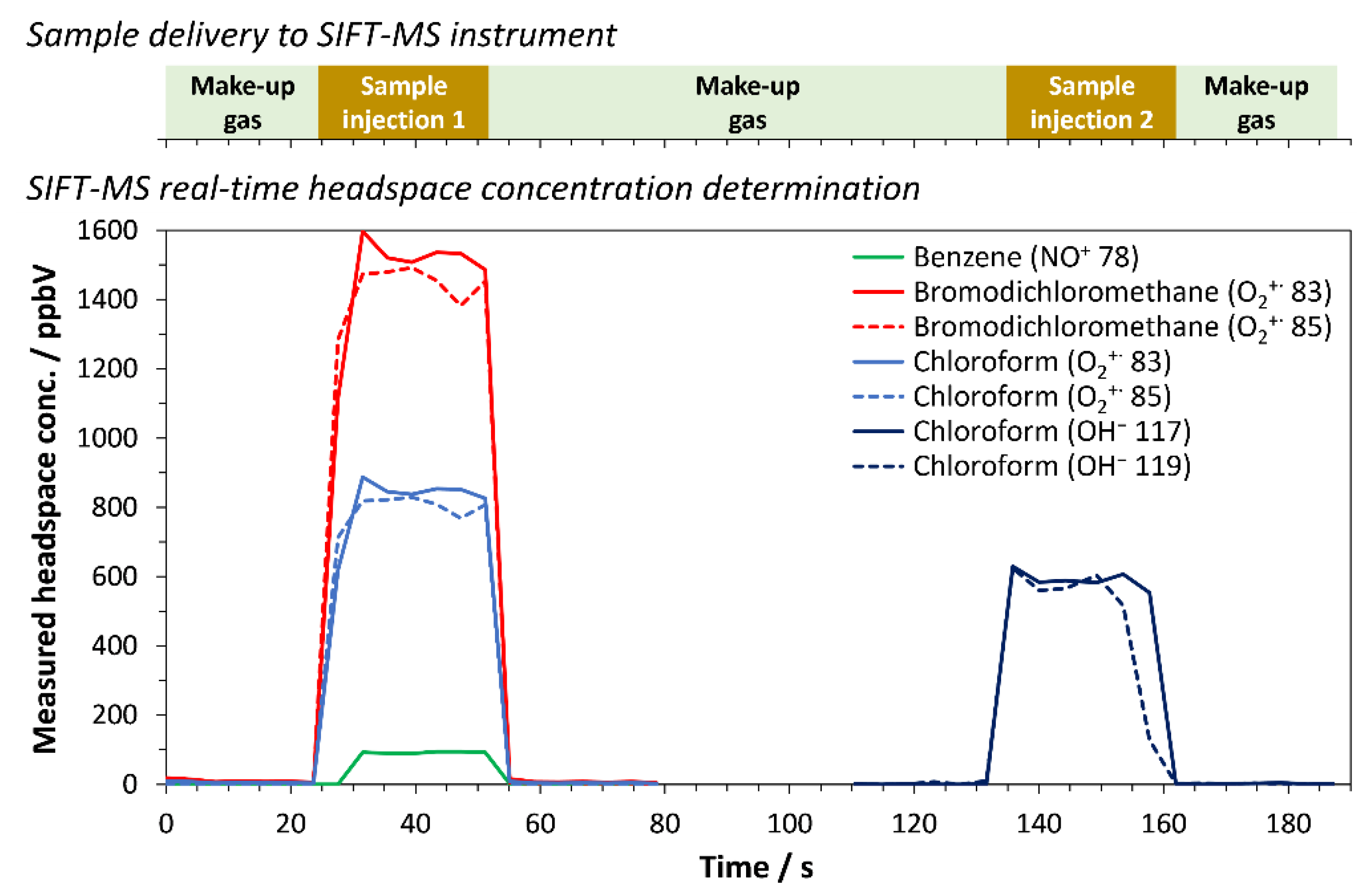
2.3.1. SIFT-MS Method
2.3.2. Headspace Analysis Optimization
3. Results
3.1. Specificity
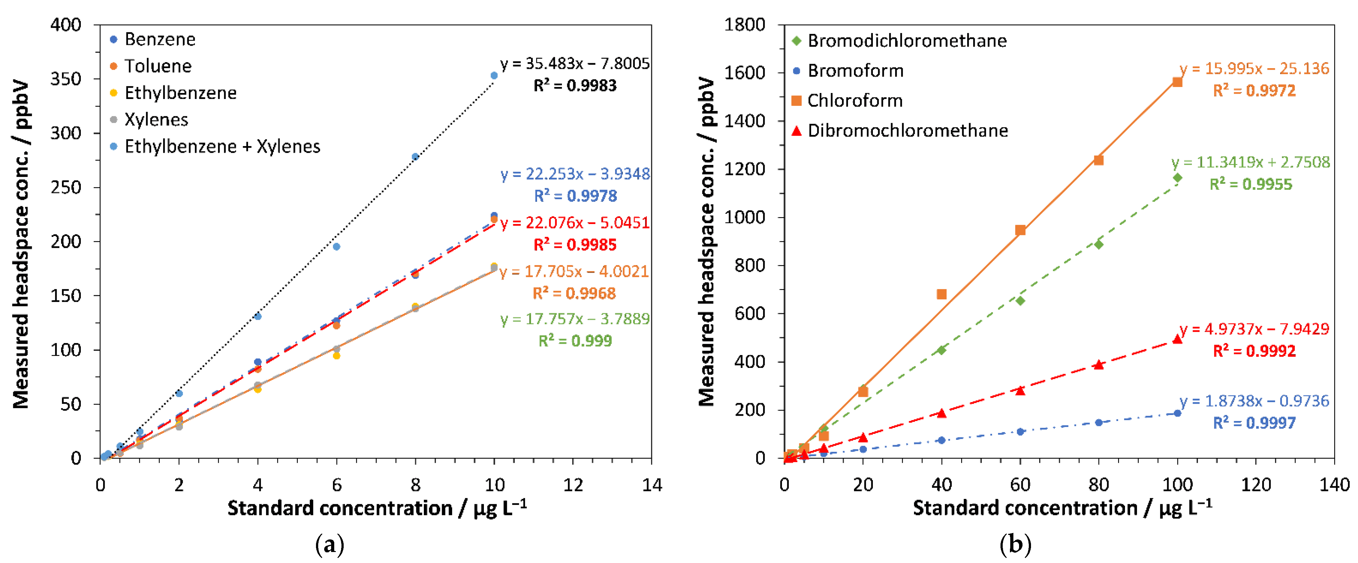
3.2. Linearity
3.3. Limit of Quantitation (LOQ) and Range
3.4. Precision
3.5. Accuracy and Recovery
3.6. Robustness
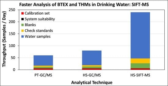
4. Discussion
Supplementary Materials
Author Contributions
Funding
Data Availability Statement
Conflicts of Interest
References
- United States Government. Code of Federal Regulations: Title 40, Part 141—National Primary Drinking Water Regulations (40 FR 59570. 1975. Available online: https://www.ecfr.gov/current/title-40/chapter-I/subchapter-D/part-141 (accessed on 8 July 2022).
- European Union. Directive (EU) 2020/2184 of the European Parliament and of the Council of 16 December 2020 on the quality of water intended for human consumption (recast) (Text with EEA relevance). Off. J. Eur. Union 2020, L 435, 1–62. Available online: https://eur-lex.europa.eu/eli/dir/2020/2184/oj (accessed on 8 July 2022).
- United States Environmental Protection Agency. National Primary Drinking Water Regulations. 2022. Available online: https://www.epa.gov/ground-water-and-drinking-water/national-primary-drinking-water-regulations (accessed on 8 July 2022).
- United States Environmental Protection Agency. National Primary Drinking Water Regulations. EPA 816-F-09-004; Maximum Contaminant Level (MCL). 2009. Available online: https://www.epa.gov/sites/default/files/2016-06/documents/npwdr_complete_table.pdf (accessed on 8 July 2022).
- United States Environmental Protection Agency. Method 524.3, Revision 1: Measurement of Purgeable Organic Compounds in Water by Capillary Column Gas Chromatography/Mass Spectrometry, EPA 815-B-09-009. 2009. Available online: https://www.nemi.gov/methods/method_summary/10417/ (accessed on 8 July 2022).
- United States Environmental Protection Agency. Method 524.4, Revision 1: Measurement of Purgeable Organic Compounds in Water by Gas Chromatography/Mass Spectrometry Using Nitrogen Purge Gas, EPA 815-R-13-002. 2013. Available online: https://www.regulations.gov/document/EPA-HQ-OW-2013-0300-0065 (accessed on 8 July 2022).
- Perkins, M.J.; Langford, V.S. Application of routine analysis procedures to a direct mass spectrometry technique: Selected ion flow tube mass spectrometry (SIFT-MS). Rev. Sep. Sci. 2021, 3, e21003. [Google Scholar] [CrossRef]
- McEwan, M.J. Direct analysis mass spectrometry. In Ion Molecule Attachment Reactions: Mass Spectrometry; Fujii, T., Ed.; Springer: New York, NY, USA, 2015; pp. 263–317. [Google Scholar]
- Taylor, A.J.; Beauchamp, J.D.; Langford, V.S. Non-destructive and high-throughput—APCI-MS, PTR-MS and SIFT-MS as methods of choice for exploring flavor release. In Dynamic Flavor: Capturing Aroma Release Using Real-Time Mass Spectrometry; Beauchamp, J.D., Ed.; American Chemical Society: Washington DC, USA, 2021; pp. 1–16. [Google Scholar] [CrossRef]
- Beale, R.; Liss, P.S.; Dixon, J.L.; Nightingale, P.D. Quantification of oxygenated volatile organic compounds in seawater by membrane inlet proton transfer reaction/mass spectrometry. Anal. Chim. Acta 2011, 706, 128–134. [Google Scholar] [CrossRef] [PubMed]
- Zou, X.; Kang, M.; Li, A.-Y.; Shen, C.-Y.; Chu, Y.-N. Spray inlet proton transfer reaction mass spectrometry (SI-PTR-MS) for rapid and sensitive online monitoring of benzene in water. Anal. Chem. 2016, 88, 3144–3148. [Google Scholar] [CrossRef]
- Zou, X.; Kang, M.; Wang, H.; Huang, C.; Shen, C.; Chu, Y. Rapid and sensitive on-line monitoring 6 different kinds of volatile organic compounds in aqueous samples by spray inlet proton transfer reaction mass spectrometry (SI-PTR-MS). Chemosphere 2017, 177, 217–223. [Google Scholar] [CrossRef]
- Alexandrou, L.D.; Meehan, B.J.; Morrison, P.D.; Jones, O.A.H. A new method for the fast analysis of trihalomethanes in tap and recycled waters using headspace gas chromatography with micro-electron capture detection. Int. J. Environ. Res. Public Health 2017, 14, 527. [Google Scholar] [CrossRef]
- Hastie, C.; Thompson, A.; Perkins, M.J.; Langford, V.S.; Eddleston, M.; Homer, N. Selected ion flow tube-mass spectrometry (SIFT-MS) as an alternative to gas chromatography/mass spectrometry (GC/MS) for the analysis of cyclohexanone and cyclohexanol in plasma. ACS Omega 2021, 6, 32818–32822. [Google Scholar] [CrossRef]
- Perkins, M.J.; Langford, V.S. Multiple headspace extraction-selected ion flow tube mass spectrometry (MHE-SIFT-MS). Part 1: A protocol for method development and transfer to routine analysis. Rev. Sep. Sci. 2022, 4, e22001. [Google Scholar] [CrossRef]
- Perkins, M.J.; Langford, V.S.; McEwan, M.J. High-throughput analysis of volatile compounds in air, water and soil using SIFT-MS. Curr. Trends. Mass. Spectrom. 2018, 37, 24–29. [Google Scholar]
- Lee, S.-H.; Shin, E.-J.; Zoh, K.-D.; Kang, Y.-S.; Choi, J.-W. Direct mass spectrometry with online headspace sample pretreatment for continuous water quality monitoring. Water 2020, 12, 1843. [Google Scholar] [CrossRef]
- Perkins, M.J.; Langford, V.S. Standard validation protocol for selected ion flow tube mass spectrometry methods applied to direct headspace analysis of aqueous volatile organic compounds. Anal Chem. 2021, 93, 8386–8392. [Google Scholar] [CrossRef] [PubMed]
- Florida Department of Environmental Protection. Chapter 62-302: Surface Water Quality Standards. Available online: https://www.epa.gov/sites/default/files/2014-12/documents/fl_section62-302.pdf (accessed on 29 August 2022).
- Smith, D.; Španěl, P. Selected ion flow tube mass spectrometry (SIFT-MS) for on-line trace gas analysis. Mass Spec. Rev. 2005, 24, 661–700. [Google Scholar] [CrossRef] [PubMed]
- Smith, D.; McEwan, M.J.; Španěl, P. Understanding gas phase ion chemistry is the key to reliable selected ion flow tube-mass spectrometry analyses. Anal. Chem. 2020, 92, 12750–12762. [Google Scholar] [CrossRef] [PubMed]
- Hera, D.; Langford, V.S.; McEwan, M.J.; McKellar, T.I.; Milligan, D.B. Negative reagent ions for real time detection using SIFT-MS. Environments 2017, 4, 16. [Google Scholar] [CrossRef]
- Prince, B.J.; Milligan, D.B.; McEwan, M.J. Application of selected ion flow tube mass spectrometry to real-time atmospheric monitoring. Rapid Commun. Mass Spectrom. 2010, 24, 1763–1769. [Google Scholar] [CrossRef]
- Wagner, R.L.; Farren, N.J.; Davison, J.; Young, S.; Hopkins, J.R.; Lewis, A.C.; Carslaw, D.C.; Shaw, M.D. Application of a mobile laboratory using a selected-ion flow-tube mass spectrometer (SIFT-MS) for characterisation of volatile organic compounds and atmospheric trace gases. Atmos. Meas. Tech. 2021, 14, 6083–6100. [Google Scholar] [CrossRef]
- Milligan, D.B.; Francis, G.J.; Prince, B.J.; McEwan, M.J. Demonstration of selected ion flow tube MS detection in the parts per trillion range. Anal. Chem. 2007, 79, 2537–2540. [Google Scholar] [CrossRef] [PubMed]
- Španěl, P.; Smith, D. SIFT studies of the reactions of H3O+, NO+ and O2+• with several aromatic and aliphatic hydrocarbons. Int. J. Mass Spectrom. 1998, 181, 1–10. [Google Scholar] [CrossRef]
- Syft Technologies Limited. SIFT-MS Compound Library; Syft Technologies Limited: Christchurch, New Zealand, 2013. [Google Scholar]
- Španěl, P.; Smith, D. Selected ion flow tube studies of the reactions of H3O+, NO+, and O2+• with some chloroalkanes and chloroalkenes. Int. J. Mass Spectrom. 1999, 184, 175–181. [Google Scholar] [CrossRef]
- Perkins, M. Speciation of Dichloromethane and Chloroform Using Negative Ion SIFT-MS, Anatune Application Note AS233. 2020. Available online: https://anatune.co.uk/application-notes/speciation-of-dichloromethane-and-chloroform-using-negative-ion-sift-ms/ (accessed on 2 July 2022).
- Thomas, R.; Liu, Y.; Mayhew, C.A.; Peverall, R. Selected ion flow tube studies of the gas phase reactions of O−, O2− and OH− with a variety of brominated compounds. Int. J. Mass Spectrom. Ion Proc. 1996, 155, 163–183. [Google Scholar] [CrossRef]
- Španěl, P.; Smith, D. Advances in On-line Absolute Trace Gas Analysis by SIFT-MS. Curr. Anal. Chem. 2013, 9, 525–539. [Google Scholar] [CrossRef]
- Smith, D.; Španěl, P. Ambient analysis of trace compounds in gaseous media by SIFT-MS. Analyst 2011, 136, 2009–2032. [Google Scholar] [CrossRef] [PubMed]
- Langford, V.S.; Billiau, C.; McEwan, M.J. Evaluation of the efficacy of SIFT-MS for speciation of wastewater treatment plant odors in parallel with human sensory analysis. Environments 2020, 7, 90. [Google Scholar] [CrossRef]
- Hua, G.; Yeats, S. Control of trihalomethanes in wastewater treatment. Fla. Water Res. J. 2010, 4, 6–12. [Google Scholar]
- Baumbach, J.I.; Stelemann, S.; Xie, Z.; Schmidt, H. Detection of the gasoline components methyl tert-butyl ether, benzene, toluene, and m-xylene using ion mobility spectrometers with a radioactive and UV ionization source. Anal. Chem. 2003, 75, 1483–1490. [Google Scholar] [CrossRef]
- Bettenhausen, C.A. Finding benzene everywhere we look. Chem. Eng. News 2022, 100, 24–26. [Google Scholar] [CrossRef]

| Name | CAS No. | EU Limit [2] | US Limit [1] | Florida Limit [19] | Supplier | Purity |
|---|---|---|---|---|---|---|
| Benzene | 71-43-2 | 1 | 5 | 2 | Fluka (St. Louis, MO, USA) | >99.9% |
| Ethylbenzene | 100-41-4 | N/A | 700 | 80 | Sigma Aldrich (St. Louis, MO, USA) | 99.8% |
| Toluene | 108-88-3 | N/A | 1000 | 56 | Aldrich | 99% |
| Xylene (sum of isomers; m- used *) | 108-38-3 | N/A | 10,000 | N/A | Sigma Aldrich | >99% |
| Bromodichloromethane | 75-27-4 | ** | 0 *** | 2.1 | Sigma Aldrich | ≥97% |
| Bromoform | 75-25-2 | ** | 0 *** | 15 | Sigma Aldrich | 99% |
| Chloroform | 67-66-3 | ** | 70 *** | 60 | Sigma Aldrich | >99% |
| Dibromochloromethane | 124-48-1 | ** | 60 *** | 1.8 | Sigma Aldrich | 98% |
| Compound, Molecular Formula | Reagent Ion | Product Ion m/z | Product Ion Formula | Ion Signal Ratios | Reference |
|---|---|---|---|---|---|
| Benzene, C6H6 | NO+ | C6H6+ | 78 | 76% | [26] |
| Bromodichloromethane, CHBrCl2 | O2+• | CH35Cl2+ | 83 | 56% | This work |
| O2+• | CH35Cl37Cl+ | 85 | 38% | This work | |
| Bromoform, CHBr3 | O2+• | CH79Br2+ | 171 | 25% | [27] |
| O2+• | CH79Br81Br+ | 173 | 50% | [27] | |
| O2+• | CH81Br2+ | 175 | 25% | [27] | |
| Chloroform, CHCl3 | O2+• | CH35Cl2+ | 83 | 56% | [28] |
| O2+• | CH35Cl37Cl+ | 85 | 38% | [28] | |
| OH− | C35Cl3+ | −117 | 42% | [29] | |
| OH− | C35Cl237Cl+ | −119 | 42% | [29] | |
| Dibromochloromethane, CHBr2Cl | O2+• | CH79Br 35Cl+ | 127 | 38% | This work |
| O2+• | CH35Cl37Cl+ | 129 | 50% | This work | |
| Ethylbenzene, C8H10 | NO+ | C8H10+ | 106 | 100% | [26] |
| O2+• | C7H7+ | 91 | 70% | [26] | |
| O2+• | C8H10+ | 106 | 30% | [26] | |
| Toluene, C7H7 | NO+ | C7H8+ | 92 | 100% | [26] |
| Xylene (all isomers; m- used), C8H10 | NO+ | C8H10+ | 106 | 100% | [26] |
| O2+• | C7H7+ | 91 | 20% | [26] | |
| O2+• | C8H10+ | 106 | 80% | [26] |
| Parameter | General-Purpose Aqueous Headspace Analysis [18] | High-Sensitivity Aqueous Headspace Analysis (This Study) |
|---|---|---|
| SIFT-MS sample analysis time | 240 s | 190 s |
| SIFT-MS product ion dwell time | 200 ms | 200 ms |
| Incubation time | 20 min | 20 min |
| Incubation temperature | 60 °C | 75 °C |
| Vial size | 20 mL | 20 mL |
| Volume of aqueous used | 10 mL | 10 mL |
| Headspace syringe volume | 2.5 mL (2 injections) ** | 2.5 mL (2 injections) ** |
| Syringe temperature | 150 °C | 150 °C |
| Headspace injection rate | 50 μL s−1 | 100 μL s−1 |
| Add NaCl | 10% (1 g in 10 mL) | 10% (1 g in 10 mL) |
| Quality control | Single point analysis, with cross-checks as required (6 repl. calibration standards at 1 ppm solution) | Single point analysis, with cross-checks as required (3 repl. calibration standards at 5 or 50 µg L−1 for BTEX or THMs, respectively |
| Solution Conc./μg L−1 | Replicate No./Statistical Parameter | Benzene | Toluene | Ethylbenzene * | Xylenes * |
|---|---|---|---|---|---|
| 0.1 | 1 | 0.810 | 0.990 | 0.720 | 0.730 |
| 2 | 0.880 | 0.530 | 0.727 | 0.595 | |
| 3 | 1.08 | 0.820 | 0.570 | 0.530 | |
| Mean | 0.923 | 0.780 | 0.672 | 0.619 | |
| SD | 0.114 | 0.190 | 0.073 | 0.083 | |
| %RSD | 12.4 | 24.3 | 10.8 | 13.5 | |
| 0.2 | 1 | 3.31 | 2.26 | 2.04 | 1.46 |
| 2 | 3.40 | 1.98 | 2.39 | 1.45 | |
| 3 | 2.79 | 2.08 | 2.24 | 1.59 | |
| Mean | 3.17 | 2.11 | 2.22 | 1.50 | |
| SD | 0.269 | 0.116 | 0.146 | 0.062 | |
| %RSD | 8.5 | 5.5 | 6.6 | 4.2 | |
| 0.5 | 1 | 4.53 | 4.63 | 2.71 | 3.32 |
| 2 | 3.94 | 3.89 | 3.34 | 3.45 | |
| 3 | 4.29 | 4.07 | 2.81 | 3.01 | |
| Mean | 4.25 | 4.20 | 2.95 | 3.26 | |
| SD | 0.242 | 0.315 | 0.277 | 0.186 | |
| %RSD | 5.7 | 7.5 | 9.4 | 5.7 |
| Solution Conc./μg L−1 | Replicate No./Statistical Parameter | Bromodichloromethane * | Bromoform | Chloroform | Dibromochloromethane |
|---|---|---|---|---|---|
| 1 | 1 | 24.3 | 0.207 | 7.12 | 2.35 |
| 2 | 33.4 | 2.02 | 6.77 | 2.20 | |
| 3 | 31.6 | 0.877 | 7.27 | 1.38 | |
| Mean | 29.8 | 1.03 | 7.05 | 1.97 | |
| SD | 3.94 | 0.747 | 0.209 | 0.424 | |
| %RSD | 13.2 | 72.3 | 3.0 | 21.5 | |
| 2 | 1 | 22.0 | 3.17 | 15.6 | 4.57 |
| 2 | 21.7 | 3.13 | 16.7 | 5.45 | |
| 3 | 18.4 | 2.76 | 15.1 | 5.14 | |
| Mean | 20.7 | 3.02 | 15.8 | 5.05 | |
| SD | 1.61 | 0.184 | 0.674 | 0.365 | |
| %RSD | 7.8 | 6.1 | 4.3 | 7.2 | |
| 5 | 1 | 36.9 | 6.69 | 33.8 | 15.3 |
| 2 | 44.2 | 6.79 | 32.6 | 17.0 | |
| 3 | 34.1 | 6.97 | 35.0 | 15.6 | |
| Mean | 38.4 | 6.81 | 33.8 | 16.0 | |
| SD | 4.27 | 0.115 | 0.959 | 0.741 | |
| %RSD | 11.1 | 1.7 | 2.8 | 4.6 |
| Solution Conc./μg L−1 | Replicate No./Statistical Parameter | Benzene | Toluene | Ethylbenzene * | Xylenes * |
|---|---|---|---|---|---|
| 1 | 1 | 17.2 | 16.4 | 13.3 | 11.7 |
| 2 | 15.8 | 15.3 | 13.3 | 12.5 | |
| 3 | 13.2 | 13.2 | 10.9 | 11.7 | |
| 4 | 14.9 | 15.1 | 13.1 | 11.8 | |
| 5 | 16.4 | 14.8 | 12.1 | 13.3 | |
| 6 | 15.4 | 15.5 | 11.2 | 12.4 | |
| Mean | 15.5 | 15.0 | 12.3 | 12.2 | |
| SD | 1.25 | 0.964 | 0.980 | 0.579 | |
| %RSD | 8.1 | 6.4 | 8.0 | 4.7 | |
| 5 | 1 | 95.9 | 94.8 | 74.4 | 79.9 |
| 2 | 98.8 | 100 | 80.7 | 77.3 | |
| 3 | 109 | 106 | 94.7 | 85.9 | |
| 4 | 97.8 | 104 | 77.0 | 82.3 | |
| 5 | 110 | 104 | 78.0 | 80.7 | |
| 6 | 102 | 108 | 81.3 | 77.8 | |
| Mean | 102 | 103 | 81.0 | 80.6 | |
| SD | 5.36 | 4.48 | 6.56 | 2.91 | |
| %RSD | 5.2 | 4.3 | 8.1 | 3.6 | |
| 9 | 1 | 196 | 197 | 158 | 156 |
| 2 | 196 | 192 | 160 | 158 | |
| 3 | 171 | 178 | 143 | 135 | |
| 4 | 201 | 199 | 157 | 157 | |
| 5 | 187 | 188 | 153 | 154 | |
| 6 | 209 | 205 | 162 | 165 | |
| Mean | 193 | 194 | 155 | 154 | |
| SD | 12.0 | 8.63 | 6.25 | 9.20 | |
| %RSD | 6.2 | 4.5 | 4.0 | 6.0 |
| Solution Conc./μg L−1 | Replicate No./Statistical Parameters | Bromodichloromethane * | Bromoform | Chloroform | Dibromochloromethane |
|---|---|---|---|---|---|
| 10 | 1 | 131 | 13.8 | 91.4 | 38.3 |
| 2 | 96.3 | 14.5 | 94.8 | 37.8 | |
| 3 | 108 | 12.5 | 85.4 | 34.8 | |
| 4 | 106 | 13.7 | 92.7 | 34.7 | |
| 5 | 107 | 13.5 | 89.3 | 37.7 | |
| 6 | 95.7 | 14.4 | 95.2 | 40.2 | |
| Mean | 107.3 | 13.7 | 91.5 | 37.2 | |
| SD | 11.7 | 0.647 | 3.39 | 1.96 | |
| %RSD | 10.9 | 4.7 | 3.7 | 5.3 | |
| 50 | 1 | 575 | 90.4 | 708 | 230 |
| 2 | 559 | 85.2 | 732 | 229 | |
| 3 | 666 | 105 | 737 | 280 | |
| 4 | 534 | 85.7 | 721 | 239 | |
| 5 | 721 | 88.4 | 740 | 254 | |
| 6 | 663 | 94.0 | 771 | 263 | |
| Mean | 620 | 91.4 | 735 | 249 | |
| SD | 67.4 | 6.63 | 19.5 | 18.7 | |
| %RSD | 10.9 | 7.3 | 2.7 | 7.5 | |
| 90 | 1 | 868 | 162 | 1458 | 428 |
| 2 | 1043 | 153 | 1373 | 434 | |
| 3 | 878 | 151 | 1108 | 382 | |
| 4 | 1030 | 154 | 1353 | 443 | |
| 5 | 820 | 155 | 1408 | 414 | |
| 6 | 1132 | 163 | 1478 | 477 | |
| Mean | 962 | 157 | 1363 | 430 | |
| SD | 113 | 4.47 | 122 | 28.7 | |
| %RSD | 11.7 | 2.9 | 9.0 | 6.7 |
| Amount/ μg L−1 | Benzene | Toluene | Ethylbenzene * | Xylenes * | Bromodichloromethane ** | Bromoform | Chloroform | Dibromochloromethane |
|---|---|---|---|---|---|---|---|---|
| Repl. 1 | <LOQ | <LOQ | <LOQ | <LOQ | 2.41 | 8.25 | <LOQ | 3.94 |
| Repl. 2 | 0.20 | <LOQ | <LOQ | <LOQ | 2.39 | 9.45 | <LOQ | 4.78 |
| Repl. 3 | <LOQ | <LOQ | <LOQ | <LOQ | 6.51 | 7.62 | <LOQ | 4.49 |
| Repl. 4 | <LOQ | <LOQ | <LOQ | <LOQ | 2.43 | 9.14 | <LOQ | 4.26 |
| Repl. 5 | <LOQ | <LOQ | <LOQ | <LOQ | 2.03 | 8.85 | <LOQ | 4.00 |
| Repl. 6 | <LOQ | <LOQ | <LOQ | <LOQ | <LOQ | 8.74 | <LOQ | 3.78 |
| Mean | N/A | N/A | N/A | N/A | 2.93 | 8.67 | N/A | 4.21 |
| SD | N/A | N/A | N/A | N/A | 1.66 | 0.83 | N/A | 0.42 |
| %RSD | N/A | N/A | N/A | N/A | 56.9 | 9.7 | N/A | 9.8 |
| Solution Conc./μg L−1 | Replicate No./Statistical Parameter | Benzene | Toluene | Ethylbenzene * | Xylenes * |
|---|---|---|---|---|---|
| 2.5 | 1 | 2.29 | 2.09 | 2.05 | 2.30 |
| 2 | 2.15 | 1.92 | 2.03 | 2.02 | |
| 3 | 2.26 | 2.02 | 2.14 | 2.12 | |
| Mean | 2.24 | 2.01 | 2.07 | 2.15 | |
| SD | 0.060 | 0.067 | 0.047 | 0.12 | |
| %RSD | 2.7 | 3.3 | 2.3 | 5.4 | |
| 5.0 | 1 | 4.81 | 4.83 | 4.37 | 5.18 |
| 2 | 4.66 | 4.18 | 4.61 | 4.97 | |
| 3 | 4.20 | 3.72 | 4.01 | 3.95 | |
| Mean | 4.56 | 4.24 | 4.33 | 4.70 | |
| SD | 0.26 | 0.45 | 0.25 | 0.54 | |
| %RSD | 5.7 | 10.7 | 5.7 | 11.5 | |
| 7.5 | 1 | 7.18 | 6.68 | 7.39 | 7.31 |
| 2 | 6.83 | 6.48 | 6.49 | 7.10 | |
| 3 | 7.24 | 6.68 | 6.57 | 7.88 | |
| Mean | 7.08 | 6.62 | 6.82 | 7.43 | |
| SD | 0.18 | 0.094 | 0.41 | 0.33 | |
| %RSD | 2.5 | 1.4 | 5.9 | 4.4 |
| Solution Conc./μg L−1 | Replicate No./Statistical Parameter | Bromodichloromethane * | Bromoform | Chloroform | Dibromochloromethane |
|---|---|---|---|---|---|
| 25 | 1 | 29.3 | 37.5 | 23.5 | 32.2 |
| 2 | 35.0 | 46.0 | 19.6 | 33.9 | |
| 3 | 30.4 | 33.9 | 21.1 | 29.9 | |
| Mean | 31.6 | 39.1 | 21.4 | 32.0 | |
| SD | 2.56 | 5.33 | 1.61 | 1.67 | |
| %RSD | 8.3 | 13.5 | 7.6 | 5.2 | |
| 50 | 1 | 112.2 ** | 64.4 | 29.8 ** | 58.6 |
| 2 | 59.2 | 62.0 | 45.6 | 53.6 | |
| 3 | 39.4 | 51.5 | 42.7 | 47.7 | |
| Mean | 70.3 | 59.3 | 39.4 | 53.3 | |
| SD | 30.7 | 5.69 | 6.86 | 4.56 | |
| %RSD | 43.7 | 9.6 | 17.4 | 8.6 | |
| 75 | 1 | 89.9 | 87.5 | 69.9 | 79.8 |
| 2 | 83.7 | 77.8 | 65.9 | 72.6 | |
| 3 | 86.4 | 77.0 | 70.4 | 79.8 | |
| Mean | 86.7 | 80.8 | 68.8 | 77.4 | |
| SD | 4.11 | 4.90 | 2.23 | 4.76 | |
| %RSD | 4.7 | 6.0 | 3.3 | 6.1 |
| Solution Conc./μg L−1 | Replicate No./Statistical Parameter | Benzene | Toluene | Ethylbenzene * | Xylenes * |
|---|---|---|---|---|---|
| 2.5 | 1 | 91.8 | 83.5 | 81.8 | 92.0 |
| 2 | 86.2 | 77.0 | 81.2 | 80.7 | |
| 3 | 90.4 | 80.9 | 85.5 | 84.9 | |
| Mean | 89.5 | 80.5 | 82.8 | 85.9 | |
| SD | 2.4 | 2.7 | 1.9 | 4.6 | |
| %RSD | 2.7 | 3.3 | 2.3 | 5.4 | |
| 5.0 | 1 | 96.2 | 96.6 | 87.4 | 103.7 |
| 2 | 93.3 | 83.5 | 92.2 | 99.4 | |
| 3 | 84.1 | 74.4 | 80.2 | 79.0 | |
| Mean | 91.2 | 84.8 | 86.6 | 94.0 | |
| SD | 5.2 | 9.1 | 5.0 | 10.8 | |
| %RSD | 5.7 | 10.7 | 5.7 | 11.5 | |
| 7.5 | 1 | 95.7 | 89.1 | 98.5 | 97.4 |
| 2 | 91.0 | 86.5 | 86.6 | 94.7 | |
| 3 | 96.5 | 89.1 | 87.6 | 105.0 | |
| Mean | 94.4 | 88.2 | 90.9 | 99.1 | |
| SD | 2.4 | 1.3 | 5.4 | 4.4 | |
| %RSD | 2.5 | 1.4 | 5.9 | 4.4 |
| Solution Conc./μg L−1 | Replicate No./Statistical Parameter | Bromodichloromethane * | Bromoform | Chloroform | Dibromochloromethane |
|---|---|---|---|---|---|
| 25 | 1 | 105.7 | 115.2 | 92.8 | 112.1 |
| 2 | 128.3 | 149.2 | 77.0 | 118.8 | |
| 3 | 109.9 | 100.9 | 83.3 | 102.9 | |
| Mean | 114.6 | 121.8 | 84.4 | 111.3 | |
| SD | 9.8 | 20.2 | 6.5 | 6.5 | |
| %RSD | 8.6 | 16.6 | 7.7 | 5.8 | |
| 50 | 1 | 218.4 ** | 111.4 | 59.0 ** | 108.7 |
| 2 | 112.6 | 106.7 | 90.5 | 98.7 | |
| 3 | 73.0 | 85.6 | 84.8 | 87.0 | |
| Mean | 134.7 | 101.2 | 78.1 | 98.1 | |
| SD | 61.4 | 11.2 | 13.7 | 8.9 | |
| %RSD | 45.6 | 11.1 | 17.6 | 9.0 | |
| 75 | 1 | 116.0 | 105.1 | 92.8 | 100.7 |
| 2 | 107.6 | 92.2 | 87.5 | 91.2 | |
| 3 | 111.3 | 91.1 | 93.5 | 100.8 | |
| Mean | 111.7 | 96.1 | 91.3 | 97.6 | |
| SD | 3.4 | 6.3 | 2.7 | 4.5 | |
| %RSD | 3.1 | 6.6 | 2.9 | 4.6 |
| Name | PT-GC/MS [6] * | HS-GC-μECD [13] | HS-SIFT-MS [17] | HS-SIFT-MS [18] | HS-SIFT-MS (This Study) |
|---|---|---|---|---|---|
| Benzene | 0.022 | 119 | 1.14 | 0.10 | |
| Ethylbenzene | 0.013 | 1.15 | 0.20 | ||
| Toluene | 0.034 | 133 | 1.15 | 0.10 | |
| Xylenes | 0.17, 0.037 ** | 1.16 | 0.10 | ||
| Bromodichloromethane | 0.027 | 0.32 | 1.0 | ||
| Bromoform | 0.021 | 0.47 | 110 | 2.0 | |
| Chloroform | 0.032 | 0.47 | 3.36 | 1.0 | |
| Dibromochloromethane | 0.016 | 0.35 | 2.0 |
Publisher’s Note: MDPI stays neutral with regard to jurisdictional claims in published maps and institutional affiliations. |
© 2022 by the authors. Licensee MDPI, Basel, Switzerland. This article is an open access article distributed under the terms and conditions of the Creative Commons Attribution (CC BY) license (https://creativecommons.org/licenses/by/4.0/).
Share and Cite
Perkins, M.J.; Langford, V.S. Application of Headspace-SIFT-MS to Direct Analysis of Hazardous Volatiles in Drinking Water. Environments 2022, 9, 124. https://doi.org/10.3390/environments9100124
Perkins MJ, Langford VS. Application of Headspace-SIFT-MS to Direct Analysis of Hazardous Volatiles in Drinking Water. Environments. 2022; 9(10):124. https://doi.org/10.3390/environments9100124
Chicago/Turabian StylePerkins, Mark J., and Vaughan S. Langford. 2022. "Application of Headspace-SIFT-MS to Direct Analysis of Hazardous Volatiles in Drinking Water" Environments 9, no. 10: 124. https://doi.org/10.3390/environments9100124
APA StylePerkins, M. J., & Langford, V. S. (2022). Application of Headspace-SIFT-MS to Direct Analysis of Hazardous Volatiles in Drinking Water. Environments, 9(10), 124. https://doi.org/10.3390/environments9100124