DEUFRABASE: A Simple Tool for the Evaluation of the Noise Impact of Pavements in Typical Road Geometries

Abstract

Traffic noise is considered by people as one of the most important sources of environmental discomfort. A way to limit the traffic noise is to reduce the noise emission, for example, by using specific low noise pavements, particularly in suburban areas. However, in real situations, it can be difficult to evaluate the impact of a given pavement, because it depends, for example, on the road geometry, the meteorological conditions, or the distance of the receiver position. Finally it can be difficult to select the most appropriate pavement for a given noise reduction objective. In this paper, a simple method is proposed to evaluate the noise impact of a pavement, in typical road geometries and environmental conditions. The proposed approach uses two databases, the first one based on measurements of emission spectra of road vehicles on several typical pavements, the second one made of pre-calculations of noise propagation for typical road configurations. Finally, the method is implemented in an interactive web tool, called DEUFRABASE, which allows one to obtain a fast estimation of the $L_{\mathrm{Aeq}}$ (1 h or 24 h) and $L_{\mathrm{den}}$ noise levels for various pavements and road configurations, as functions of the traffic flow and composition. By comparing the method with measurements, it is showed that the tool, although based on a restricted number of pavements and on several simplifications, can predict the noise impact of typical road configurations, with an acceptable error, most often less than 2 dB.

1. Introduction

Traffic noise is considered by people living in urban areas or next to high-trafficked suburban roads as one of the most important sources of environmental discomfort, with strong health effects [1]. Before acting on noise propagation between vehicles and housings by inserting noise barriers or reinforcing building façades, it is better to directly deal with the acoustic source for controlling and decreasing traffic noise. In this context, the development of optimized vehicle engines and road pavements, traffic management, as well as specific urban facilities, are relevant solutions [2].

In a practical point of view, the choice of a specific road pavement, in order to reach a given noise reduction at a given position (i.e., at a building facade for example), is not trivial, because it depends mainly on the road configuration, the traffic flow and composition, the nature of the soils around the road, the distance of the observation point, the meteorological conditions… The use of complex numerical methods (such as the boundary element method or the parabolic equation), although possible, is difficult to implement by road professionals, preferring faster and more functional tools, as close as possible to a practitioner’s real needs.

The present paper deals with this objective by proposing a simple and fast method to evaluate the noise impact of a given road pavement, in terms of regulatory environmental noise indicators, such as the day–evening–night A-weighted equivalent sound pressure level proposed in the European Directive 2002/49/EC, relating to the assessment and management of environmental noise [3]. The proposed approach is based on the coupling of two databases, one for describing the noise emission from several typical road pavements, and the other for applying the attenuation due to the noise propagation between the sound source and the receiver, for several road geometries and environments.

At this stage, it is important to specify that, since the subject of the study concerns the noise impact of road surfaces, the proposed methodology focuses on typical traffic flow of suburban areas, and in particular, considering vehicle speeds where rolling noise is predominant. In addition, only ‘basic’ geometries are considered, representative of national roads or motorways, in a semi-open field. The aim of the methodology detailed in the present paper is not to assess the impact of a road infrastructure on the population, particularly in urban areas, as it could be envisaged using a traditional but more complex and time consuming noise prediction method, such as the CNOSSOS method [4].

From the initial authors’ development [5], the method, which is detailed in Section 2, has been updated to provide more functionality, thanks to a new web online tool implementation called DEUFRABASE (Section 3). In addition, a deeper validation of the method is detailed (Section 4), using in situ measurements as references, showing a good behaviour of the proposed methodology.

2. Principle of the Method

The method is based on the calculation of the A-weighted equivalent sound level ($L_{\mathrm{Aeq}}$) in an open-field (including the attenuation due to the propagation in various road geometries) function of the pass-by maximum sound pressure level $L_{\mathrm{A},\max }$ that has been measured on a given pavement. It allows the calculation of the following indicators:

• $L_{\mathrm{Aeq},1\mathrm{h}}$, which is the A-weighted equivalent sound pressure level based on the 1 hour-traffic of passenger cars (PC) and heavy trucks (HT),
• $L_{\mathrm{Aeq},24\mathrm{h}}$, which is the A-weighted equivalent sound pressure level based on the traffic distribution of PC and HT over the 24 h of a day,
• $L_{\mathrm{den}}$, which is the day–evening–night A-weighted equivalent sound pressure level, calculated from the $L_{\mathrm{Aeq},24\mathrm{h}}$.

These indicators can be computed for each situation (geometry, meteorological conditions, road traffic), for different road pavements that are considered in the database, from the knowledge of some information [6]:

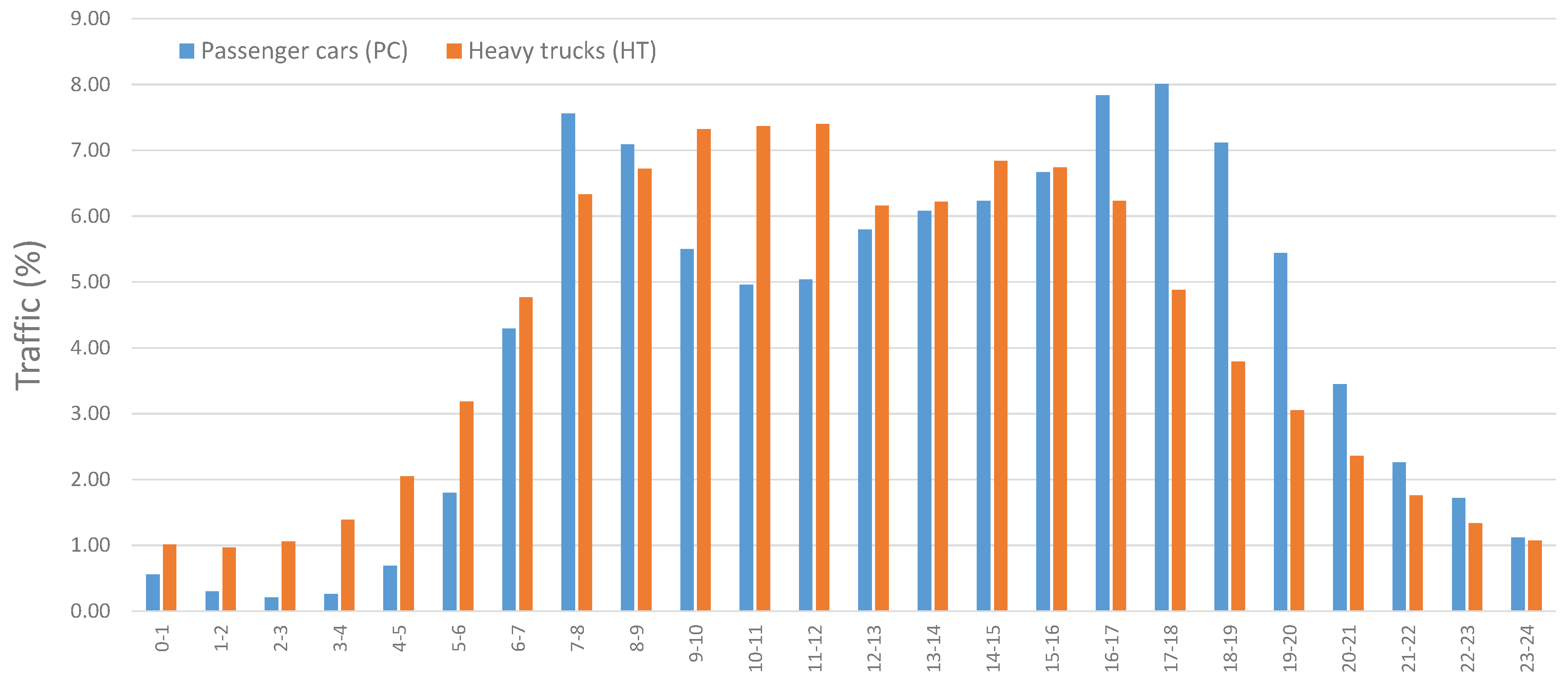
• the hourly-traffic distribution during the three periods of a full day: [6:00–18:00] for the daytime period, [18:00–22:00] for the evening period and [22:00–6:00] for the night period. In the present approach, to be as close as possible to real configurations, two main vehicle classes are considered; the passenger cars (PC) and the heavy trucks (HT), defined by their traffic distribution $n_{\mathrm{PC}}$ and $n_{\mathrm{HT}}$, respectively,
• the number and the width of traffic lanes,
• the reference speed of each vehicle class $V_{\mathrm{ref}}$ (90 or 110 km/h for PC and 80 km/h for HT),
• the A-weighted pass-by maximum sound pressure level $L_{\mathrm{A},\max }$ for PC and HT vehicles (in global and third octave values) measured at a reference microphone, according to the International Organization for Standardization (ISO) statistical pass-by (SPB) method [7] (7.50 m from the right lane axis and 1.20 m above the ground),
• typical road geometries with different ground parameters,
• different meteorological conditions.

2.1. Sound Pressure Level Calculation

A general representation of the situation can be summarized on Figure 1, where the vehicle is assumed to be an equivalent spherical point source S. Let’s consider the A-weighted pass-by maximum sound pressure level $L_{\mathrm{A},\max ,V_{\mathrm{ref}}}\left(D_{\mathrm{ref}}\right)$, measured at a reference speed $V_{\mathrm{ref}}$ and at the reference microphone $R_{\mathrm{ref}}$ located at a distance $D_{\mathrm{ref}}$ from the source S, in accordance to the ISO standard 11819-1 [7]. Thus, the A-weighted pass-by maximum sound pressure level $L_{\mathrm{A},\max ,V_{\mathrm{ref}}}\left(D_{\mathrm{obs}}\right)$ at a determined receiver $R_{\mathrm{obs}}$ (the observation point) located at a distance $D_{\mathrm{obs}}$ from the source S, can be calculated, at the same speed $V_{\mathrm{ref}}$, according to the following equation:

$$L_{\mathrm{A},\max ,V_{\mathrm{ref}}}\left(D_{\mathrm{obs}}\right)=L_{\mathrm{A},\max ,V_{\mathrm{ref}}}\left(D_{\mathrm{ref}}\right)+\mathrm{Attenuation},$$

(1)

with $D_{\mathrm{ref}}$ the distance between the reference position $R_{\mathrm{ref}}$ and the source S, defined as:

$$D_{\mathrm{ref}}=\sqrt{d_{\mathrm{ref}}^2+{\left(z_{\mathrm{ref}}-h_S\right)}^2},$$

(2)

and $D_{\mathrm{obs}}$ the distance between the observation point $R_{\mathrm{obs}}$ and the source S, defined as:

$$D_{\mathrm{obs}}=\sqrt{d_{\mathrm{obs}}^2+{\left(h_{\mathrm{obs}}-h_S\right)}^2},$$

(3)

where $d_{\mathrm{ref}/\mathrm{obs}}$ are the horizontal distances from the sound source S to the location of the reference/observation points respectively, $h_{\mathrm{obs}}$ the height of the observation point $R_{\mathrm{obs}}$ above the ground and $z_{\mathrm{ref}}$ the height of the reference receiver $R_{\mathrm{ref}}$ above the pavement.

The way to calculate the ‘attenuation’ term in Equation (1) depends on the complexity of the cross section of the road, the presence of an impedance discontinuity close to the pavement and micro-meteorological conditions [8,9]. For simple cases, for instance such as flat dense or porous ground with or without impedance discontinuity and with or without positive vertical sound celerity profile, ray tracing analytical models have been used. Using this approach, heterogeneous grounds as well as noise barriers [10] with homogeneous and favorable meteorological conditions can be easily investigated. For more complex configurations, such as embankment and depressed roads, or roads with a noise barrier, with or without impedance discontinuity, specific numerical approaches have been considered; the boundary element method (BEM) [11,12] can be applied to very complex shapes, such as a non-flat ground with a noise barrier; the parabolic equation (PE) formulation [13] is more appropriate in order to consider noise propagation above a ground with impedance discontinuities and topographical irregularities, both in a turbulent and refractive atmosphere.

The ‘attenuation’ term in Equation (1) can be expressed by the following equation:

$$\mathrm{Attenuation}=\mathrm{Attenuation}\left(R_{\mathrm{obs}}\right)-\mathrm{Attenuation}\left(R_{\mathrm{ref}}\right)-20{log}_{10}\frac{D_{\mathrm{obs}}}{D_{\mathrm{ref}}}-{\mathrm{Att}}_{\mathrm{air}}\left(D_{\mathrm{obs}}\right)+{\mathrm{Att}}_{\mathrm{air}}\left(D_{\mathrm{ref}}\right).$$

(4)

The two first ‘attenuation’ terms correspond to the attenuation due to propagation, calculated using the procedures detailed above. Due to the convention, these attenuation terms are considered as positive values. Since these attenuation terms have been calculated relatively to free field, they require to be corrected by the free field propagation (third term). The two last terms ${\mathrm{Att}}_{\mathrm{air}}$ are due to the atmospheric attenuation (temperature T = 20 °C, relative humidity H = 60%) calculated according to the ISO standard 9613-1 [14].

The ‘attenuation’ term is evaluated for typical road geometries and specific meteorological conditions (see Section 2.2.1), according to the most suitable acoustic propagation method. Results are then stored in an ’attenuation’ database, which is used later in the DEUFRABASE tool (see Section 3). This pre-calculation allows us to obtain results instantly, which would not be possible if the calculation of the attenuation had to be integrated into the tool.

Finally, the A-weighted equivalent sound level $L_{\mathrm{Aeq}}\left(R_{\mathrm{obs}}\right)$ at the receiver $R_{\mathrm{obs}}$ during a given period T can be calculated using the following equation [15], for a given PC or HT vehicle:

$$L_{\mathrm{Aeq}}\left(R_{\mathrm{obs}}\right)=L_{\mathrm{A},\max ,V_{\mathrm{ref}}}\left(D_{\mathrm{obs}}\right)+10{log}_{10}\left(\frac{\pi D_{\mathrm{obs}}}{V_{\mathrm{ref}}T}\right).$$

(5)

As suggested by the notation in this last equation, this relationship is only valid if the speed $V_{\mathrm{ref}}$, that is considered in the second right member, corresponds to the velocity of the traffic flow when measuring the $L_{\mathrm{A},\max ,V_{\mathrm{ref}}}$ (first right member). However, a speed correction is proposed at Section 3.3.2 for considering a speed that could be different than the reference ones.

The $L_{\mathrm{Aeq}}$ sound pressure level at a given receiver for a typical traffic flow of PC and HT on the three periods of a day (the day ‘d’ for $T$ = [6:00–18:00], the evening ‘e’ for $T$ = [18:00–22:00] and the night ‘n’for $T$ = [22:00–6:00]), can be obtained by summing the respective contribution of each vehicle as follow:

$$L_{\mathrm{d},\mathrm{e},\mathrm{n}}\equiv L_{\mathrm{Aeq}}[T=\mathrm{d},\mathrm{e},\mathrm{n}]=10{log}_{10}\left\{\frac{1}{T}\left(n_{\mathrm{PC}}\times {10}^{0.1\times L_{\mathrm{Aeq},\mathrm{PC}}\left[T\right]}+n_{\mathrm{HT}}\times {10}^{0.1\times L_{\mathrm{Aeq},\mathrm{HT}}\left[T\right]}\right)\right\},$$

(6)

where $n_{\mathrm{PC}/\mathrm{HT}}$ are the number of vehicles in the traffic flow during the period T and $L_{\mathrm{Aeq},\mathrm{PC}/\mathrm{HT}}$ the equivalent sound pressure levels at the receiver $R_{\mathrm{obs}}$, for the PC and HT respectively.

Afterwards, the common European noise indicator $L_{\mathrm{den}}$ [3] is obtained by summing all noise contributions on each period of the day ($L_{\mathrm{d}}$), evening ($L_{\mathrm{e}}$) and night ($L_{\mathrm{n}}$), including a weighting of $+5$ dB for the evening and $+10$ dB for the night:

$$L_{\mathrm{den}}=10{log}_{10}\left(\frac{12}{24}{10}^{0.1\times L_{\mathrm{d}}}+\frac{4}{24}{10}^{0.1\times \left(L_{\mathrm{e}}+5\right)}+\frac{8}{24}{10}^{0.1\times \left(L_{\mathrm{n}}+10\right)}\right).$$

(7)

2.2. Input Parameters

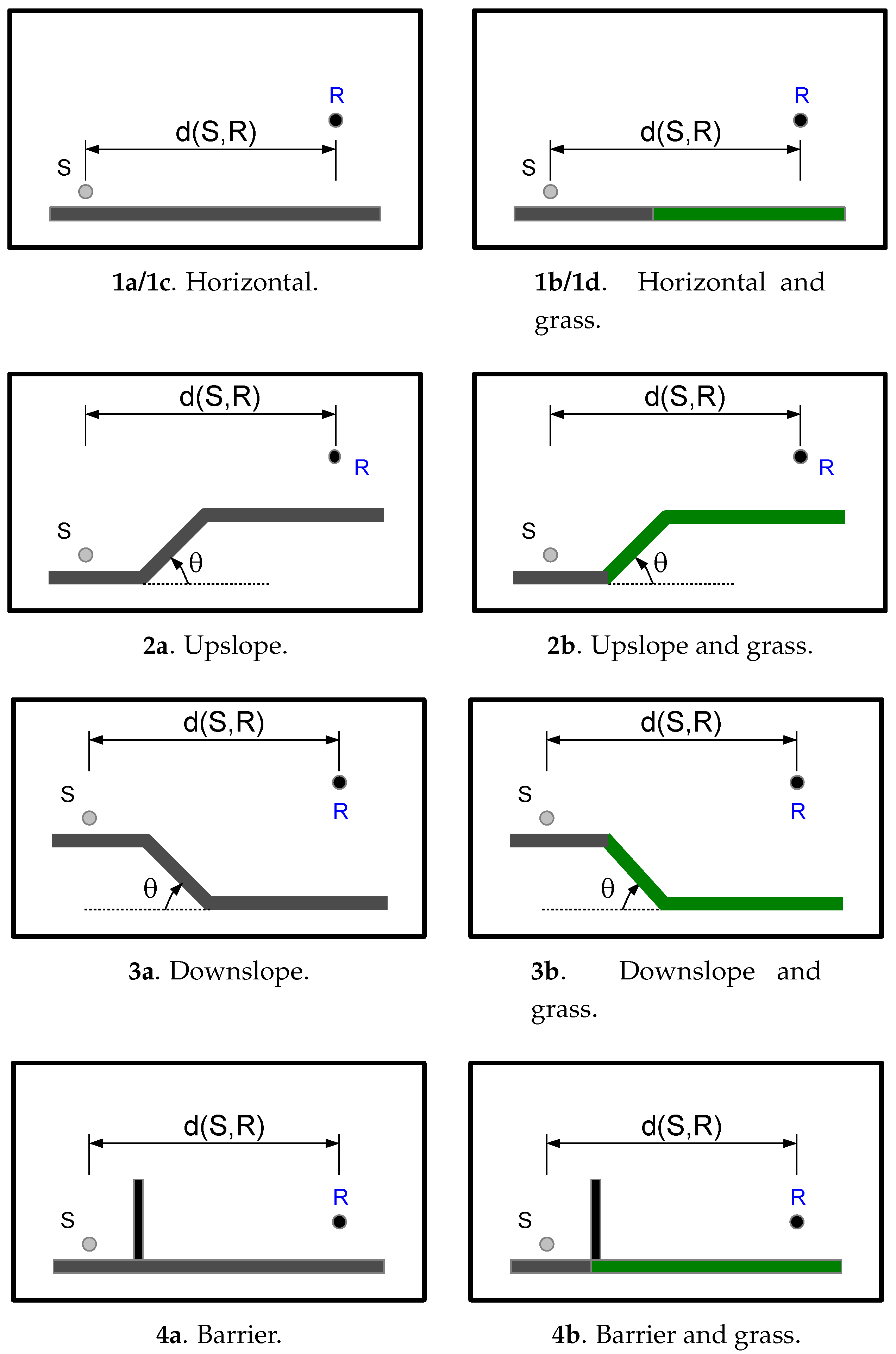
2.2.1. Road Configurations

For the results produced by the proposed tool to be relevant and usable, it is important that the available road geometries be as realistic as possible, particularly in terms of road cross-sections, neighboring grounds and meteorological conditions. Thus, eight realistic road geometries are proposed (see Figure 2 and

Table 1. Geometrical road configurations. Distances d and heights h are given in meters (m). Propagation above a ‘dense’ ($Z\to +\infty$) or ‘porous’ ($Z_{\mathrm{PA}}$) pavement, at ‘short’ (7.50 m, 50 m) or ‘long’ distances (100 m, 200 m), with ($Z_1$ and $Z_2$) or without ($Z_2=Z_1$) an impedance ‘discontinuity’; with or without ‘gradient’ (celerity profile), with or without ‘up-slope’ or ‘down-slope’ (slope defined by the angle $\theta$ and the height $h_{\mathrm{slope}}$), with or without a ‘barrier’ (height $h_{\mathrm{barrier}}$). See Figure 2 for corresponding geometries.

Geometry	${\mathit{Z}}_1$	$\mathbf{\partial }\mathit{c}/\mathbf{\partial }\mathit{h}$	${\mathit{h}}_{\mathit{R}}$	$\mathit{d}(\mathit{S},\mathit{R})$	${\mathit{Z}}_2$	$\mathit{d}(\mathit{S},\mathbf{disc})$	$\mathit{d}(\mathit{S},\mathbf{slope})$	${\mathit{h}}_{\mathbf{slope}}$	$\mathbf{\theta }$ (deg)	$\mathit{d}(\mathit{S},\mathbf{barrier})$	$\mathit{d}(\mathbf{barrier},\mathit{R})$	${\mathit{h}}_{\mathbf{barrier}}$
1a (dense, short)	$\to +\infty$	0	1.20	7.50	-	-	-	-	-	-	-	-
1a (porous, short)	$Z_{\mathrm{PA}}$	0	1.20	7.50	-	-	-	-	-	-	-	-
1b (dense, discontinuity, short)	$\to +\infty$	0	1.20	7.50	$Z_{\mathrm{grass}}$	4	-	-	-	-	-	-
1b (porous, discontinuity, short)	$Z_{\mathrm{PA}}$	0	1.20	7.50	$Z_{\mathrm{grass}}$	4	-	-	-	-	-	-
1c (dense, long)	$\to +\infty$	0	2	200	-	4	-	-	-	-	-	-
1c (dense, long, gradient)	$\to +\infty$	0.25	2	200	-	4	-	-	-	-	-	-
1c (porous, long)	$Z_{\mathrm{PA}}$	0	2	200	$Z_{\mathrm{PA}}$	4	-	-	-	-	-	-
1c (porous, long, gradient)	$Z_{\mathrm{PA}}$	0.25	2	200	$Z_{\mathrm{PA}}$	4	-	-	-	-	-	-
1d (dense, discontinuity, long)	$\to +\infty$	0	2	200	$Z_{\mathrm{grass}}$	4	-	-	-	-	-	-
1d (dense, discontinuity, long, gradient)	$\to +\infty$	0.25	2	200	$Z_{\mathrm{grass}}$	4	-	-	-	-	-	-
1d (porous, discontinuity, long)	$Z_{\mathrm{PA}}$	0	2	200	$Z_{\mathrm{grass}}$	4	-	-	-	-	-	-
1d (porous, discontinuity, long, gradient)	$Z_{\mathrm{PA}}$	0.25	2	200	$Z_{\mathrm{grass}}$	4	-	-	-	-	-	-
2a (dense, upslope, short)	$\to +\infty$	0	2	50	-	-	-	-	-	-	-	-
2a (dense, upslope, long, gradient)	$\to +\infty$	0.25	2	100	-	-	-	-	-	-	-	-
2b (dense, discontinuity, upslope, short)	$\to +\infty$	0	2	50	$Z_{\mathrm{grass}}$	4	4	+1.5	8	-	-	-
2b (dense, discontinuity, upslope, long, gradient)	$\to +\infty$	0.25	2	100	$Z_{\mathrm{grass}}$	4	4	+1.5	8	-	-	-
2b (porous, discontinuity, upslope, short)	$Z_{\mathrm{PA}}$	0	2	50	$Z_{\mathrm{grass}}$	4	4	+1.5	8	-	-	-
2b (porous, discontinuity, upslope, long, gradient)	$Z_{\mathrm{PA}}$	0.25	2	100	$Z_{\mathrm{grass}}$	4	4	+1.5	8	-	-	-
3a (dense, downslope, short)	$\to +\infty$	0	2	50	-	-	4	-1.5	8	-	-	-
3a (dense, downslope, long, gradient)	$\to +\infty$	0.25	2	100	-	-	4	-1.5	8	-	-	-
3b (dense, downslope, discontinuity, short)	$\to +\infty$	0	2	50	$Z_{\mathrm{grass}}$	4	4	-1.5	8	-	-	-
3b (dense, downslope, discontinuity, long, gradient)	$\to +\infty$	0.25	2	100	$Z_{\mathrm{grass}}$	4	4	-1.5	8	-	-	-
3b (porous, downslope, discontinuity, short)	$Z_{\mathrm{PA}}$	0	2	50	$Z_{\mathrm{grass}}$	4	4	-1.5	8	-	-	-
3b (porous, downslope, discontinuity, long, gradient)	$Z_{\mathrm{PA}}$	0.25	2	100	$Z_{\mathrm{grass}}$	4	4	-1.5	8	-	-	-
4a (dense, barrier)	$\to +\infty$	0	3	40	-	-	-	-	-	4	36	2
4b (dense, barrier, discontinuity)	$\to +\infty$	0	3	40	$Z_{\mathrm{grass}}$	4	-	-	-	4	36	2
4b (porous, barrier, discontinuity)	$Z_{\mathrm{PA}}$	0	3	40	$Z_{\mathrm{grass}}$	4	-	-	-	4	36	2

), including acoustics propagation over a flat ground, the presence of a barrier or a down/up-slope, with or without an impedance discontinuity asphalt/grass. For long range propagation (i.e., for source-receiver distances above 100 m), a celerity profile is also considered, and corresponds to a condition favouring the propagation of noise towards the observation point (i.e., a ‘favourable’ condition for acoustic propagation, which is a penalizing condition for a resident).

Each road geometry is defined by specific acoustic absorption parameters; the ground impedance Z for locally reacting surfaces are estimated by the Delany and Bazley one-parameter ($\sigma$) model [16]. For a porous asphalt (PA) surface, the phenomenological three parameter ($\sigma$, $\Omega$ and $q^2$) model [17] is used; parameters $\sigma$, $\Omega$ and $q^2$ are the specific airflow resistivity (in kNsm⁻⁴), the porosity and the tortuosity, respectively.

In the present study, the following parameters have been considered:

• for grassy soils ($Z_{\mathrm{grass}}$): $\sigma =200$ kNsm⁻⁴,
• for porous asphalts ($Z_{\mathrm{PA}}$): $\sigma =10$ kNsm⁻⁴, $\Omega =25$%, $q^2=3.5$,
• for dense pavements, the impedance Z is considered as infinite ($Z\to +\infty$).

The source height $h_S$ is fixed to 0.05 m for all configurations, according to the estimated source height for a road vehicle [18].

Meteorological conditions are considered through the vertical sound velocity gradient $\partial c/\partial h$; $\partial c/\partial h=0$ corresponds to a homogeneous condition, occurring at sunset and sunrise periods (this condition is considered all over the daytime period); $\partial c/\partial h=0.25$ corresponds to a ‘favourable’ condition, mainly occurring during night time (rather strong effect).

2.2.2. Pavement Data

Table 2. Pavement database: $L_{\mathrm{A},\max }$ sound levels for road vehicles, at 90 or 110 km/h (PC) and 80 km/h (HT). French and German pavements are noted with the FR and GE notations respectively. The numbers after the pavement description corresponds to the minimum/maximum size of the aggregates. In addition, the ‘type’ defines the porosity properties; ‘Type 1’ means a porosity $\Omega$ lower or equal than 15% and ‘Type 2’ a porosity means $\Omega$ between 15% and 25%. As an example, ‘VTAC 0/6 Type 2’ corresponds to a very thin asphalt concrete (VTAC) with aggregate sizes between 0 and 6 mm and a porosity close to 20%.

Country	Description	Name	PC 90 km/h ${\mathit{L}}_{\mathbf{A},\mathbf{max}}$	PC 110 km/h ${\mathit{L}}_{\mathbf{A},\mathbf{max}}$	HT 80 km/h ${\mathit{L}}_{\mathbf{A},\mathbf{max}}$
FR	PA 0/6	Porous asphalt 0/6	72.8	75.4	80.3
GE	PA 0/8	Porous asphalt 0/8	79.0	81.0	85.3
GE	TLPA 0/8	Twin layer porous asphalt 0/8	75.9	77.4	81.7
FR	PA 0/10	Porous asphalt 0/10	74.2	76.8	82.0
FR	PA 0/14	Porous asphalt 0/14	76.1	78.7	83.9
FR	VTAC 0/6 – Type 1	Very thin asphalt concrete 0/6—Type 1	74.9	77.5	82.8
FR	VTAC 0/6 – Type 2	Very thin asphalt concrete 0/6—Type 2	73.4	76.0	81.4
FR	UTAC 0/6	Ultra thin asphalt concrete 0/6	74.1	76.7	83.5
FR	VTAC 0/8 – Type 1	Very thin asphalt concrete 0/8—Type 1	76.2	78.8	82.6
FR	TAC 0/10	Thin asphalt concrete 0/10	77.6	80.2	85.6
FR	VTAC 0/10 – Type 1	Very thin asphalt concrete 0/10—Type 1	79.0	81.6	85.2
FR	VTAC 0/10 – Type 2	Very thin asphalt concrete 0/10—Type 2	75.3	77.9	82.6
FR	UTAC 0/10	Ultra thin asphalt concrete 0/10	78.3	81.0	84.4
FR	VTAC 0/14	Very thin asphalt concrete 0/14	80.4	83.0	86.2
FR	DAC 0/10 (Ref)	Dense asphalt concrete 0/10	78.0	80.6	85.4
FR	DAC 0/14	Dense asphalt concrete 0/14	80.0	82.7	86.2
FR	SMA 0/5 ln	Low noise stone mastic asphalt 0/5	78.7	80.9	88.7
FR	SMA 0/8 ln	Low noise stone mastic asphalt 0/8	78.7	80.5	87.1
FR	SMA 0/8 S	Special stone mastic asphalt 0/8	80.1	81.9	85.9
GE	SMA 0/11	Stone mastic asphalt 0/11	81.8	83.9	88.3
GE	SMA 0/11 S	Special stone mastic asphalt 0/11	81.4	83.4	87.5
FR	CASS	Cold applied slurry surfacing	78.6	81.2	85.3
FR	SD 6/10	Surface dressing 6/10	80.0	82.6	85.9
FR	SD 10/14	Surface dressing 10/14	82.1	84.7	86.4
GE	GA 0/5	Mastic asphalt 0/5	81.8	83.1	88.6
GE	GA 0/5 ln	Low noise mastic asphalt 0/5	81.7	82.6	87.0
GE	CC	Cement concrete	81.2	83.8	87.5
GE	CC	Cement concrete	83.0	84.4	90.9
GE	CC 0/16 Kamm	Cement concrete treated with jute-cloth	80.9	82.7	87.9
GE	EAC 0/5	Exposed aggregate concrete 0/5	82.1	83.6	90.4
GE	EAC 0/8	Exposed aggregate concrete 0/8	82.6	84.9	88.7
GE	CCST 0/16	Cement concrete treated with synthetic turf	81.6	83.6	89.7

shows pavement surfaces that have been introduced in database of noise emission. Because the proposed method was developed in the framework of a French–German cooperation (DEUFRAKO), the database focuses on French and German typical pavements.

For building this noise database emission, the average $L_{\mathrm{A},\max }$ values (spectra in third octave bands) have been measured at the reference point (7.50 m, 1.20 m), following the standard statistical pass-by (CPB) approach [7], on several roads covered with the different pavements. In order to consider the two main road categories (national roads and highways, i.e., with suburban speeds), two average reference speeds ($V_{\mathrm{ref}}$) have been considered for the passenger cars (90 and 110 km/h), and one reference speed for the heavy trucks (80 km/h).

Although the emission database is based on relatively old noise emission measurements, most of the pavements presented in the database are still widely used, including recent renovation and construction projects. However, using the proposed tool (see Section 3), users have also the possibility to consider their own pavement information, by uploading a specific file according to a given format, which contains the noise emission spectra for both the HT and PC vehicles, at the reference speeds 80 km/h and 90/110 km/h respectively. This functionality thus makes it possible to consider new road pavements, whose acoustic properties would be very different from those of the current database, and lastly to compare it with more traditional pavements.

2.2.3. Traffic Data

In order to evaluate the hourly $L_{\mathrm{Aeq}}$ sound level, it is necessary to have hourly traffic data of passenger cars and heavy trucks. Although it is possible to use specific traffic data (see Section 3), the user also has the possibility to use typical road traffic distributions, which have been obtained on the basis of traffic measurements in France and Germany, on weekdays.

These measurements on ($2\times 1$) and ($2\times 2$) lane roads provide information on the typical distribution of vehicles on each lane (see

Table 3. Traffic classes.

Number of Vehicles per Lane	Percentage of HT	Distribution of Vehicles	Global Traffic ($2\times 1$)	Global Traffic ($2\times 2$)
20,000	10%	PC: 18,000 HT: 2000	40,000	80,000
20,000	15%	PC: 17,000 HT: 3000	40,000	80,000
10,000	10%	PC: 9000 HT: 1000	20,000	40,000
10,000	15%	PC: 8500 HT: 1500	20,000	40,000

and

Table 4. Vehicle distribution per lane.

Number of Lanes	PC Distribution per Lane	HT Distribution per Lane
($2\times 1$)	100%	100%
($2\times 2$)	Slow lane: 50% – Fast lane: 50%	Slow lane: 90% – Fast lane: 10%

), allowing to calculate the $L_{\mathrm{Aeq},1\mathrm{h}}$ sound level.

In the case of a $L_{\mathrm{Aeq},24\mathrm{h}}$ or $L_{\mathrm{den}}$ calculations, traffic data are applied over the 24 h of the day. In this case, the daily volumes of traffic (PC and HT) for each hour are defined as the average values between the German and French traffic volume, for PC and HT respectively. The average German traffic was calculated as the mean value of nine different motorway observation points, while the average French traffic is based on twenty seven observation points around the Nantes (French city) ring road. Average values for PC and HT are shown on Figure 3 and detailed at

Table 5. Average daily traffic distribution per 1 h period (in %); passenger cars (PC) and heavy trucks (HT).

Hourly Period	PC (in %)	HT (in %)
0–1	0.56	1.01
1–2	0.30	0.97
2–3	0.21	1.06
3–4	0.26	1.39
4–5	0.69	2.05
5–6	1.80	3.18
6–7	4.29	4.77
7–8	7.56	6.33
8–9	7.09	6.72
9–10	5.50	7.32
10–11	4.96	7.37
11–12	5.04	7.40
12–13	5.80	6.16
13–14	6.08	6.22
14–15	6.23	6.84
15–16	6.67	6.74
16–17	7.84	6.23
17–18	8.01	4.88
18–19	7.12	3.79
19–20	5.44	3.05
20–21	3.45	2.36
21–22	2.26	1.76
22–23	1.72	1.34
23–24	1.12	1.07
Total	100	100

. In Figure 3, one can distinguish, among other things, the morning and evening peak hours, which are quite similar in most western European countries.

3. Implementation of the Method

3.1. Calculation Tool

Since the beginning of the French–German cooperation, three releases of the method implementation (called DEUFRABASE) have been proposed. The present description concerns the last release (V3) developed by the Ifsttar institute. The main idea of the last method implementation was to propose a lightweight and efficient platform for the setup of input parameters and the rendering of results. Databases, a calculation program, and user interfaces were served through a static HyperText Transfer Protocol (HTTP) website [19]. The DEUFRABASE was made of a set of JavaScript Object Notation (JSON) files, which are human-readable and can be easily updated with a simple text editor. The calculation program was written into JavaScript, which can be interpreted by any web browser with a reasonable speed and on many operating systems. The graphical interface was written in HyperText Markup Language (HTML) and Cascading Style Sheets (CSS), which allowed an attractive and easily maintainable rendering.

In practice, the user had to follow three steps:

• select a road configuration in a list (‘Geometry’ tab of the web tool), as defined in Table 1;
• select one or more road pavements in a list (‘Pavement’ tab). The pavement list displayed depended on the selected road configuration at the first step (i.e., dense or porous road surface). At this step, the user had the possibility to consider his own noise emission data, at the condition that it respects the proposed JSON file format and the measurement conditions (CPB method). Note that the user can also consider emission data that would have been measured at other traffic speeds, by ‘bypassing’ the expected data in the file for each reference speed (for example, by associating the expected values at 90 km/h for a PC, with data measured at another speed);
• define the traffic flow and composition, as well as the number of lanes (‘Traffic’ tab). Depending the noise indicator to be calculated ($L_{\mathrm{Aeq},1\mathrm{h}}$ or $L_{\mathrm{Aeq},24\mathrm{h}}$/$L_{\mathrm{den}}$), the user had to provide the traffic distribution of a given hour or for each of the 24 h periods. At this step, the user also had the possibility to use the proposed average daily traffic distribution or his own data.

Once the three steps were completed, the results were given in terms of $L_{\mathrm{Aeq},1\mathrm{h}}$ or $L_{\mathrm{Aeq},24\mathrm{h}}$/$L_{\mathrm{den}}$. Additionally, the user could save/restore input data using a local JSON file and export results in a spreadsheet for extra processing.

3.2. General Considerations

For the sake of simplification, several points have been considered in the calculation:

• the calculation of the ‘attenuation’ term in Equation (5) between the reference receiver $R_{\mathrm{ref}}$ and the receiver $R_{\mathrm{obs}}$ located far away were always carried out with respect to the median axis of the right traffic lane,
• because the traffic is distributed among the different lanes (two or four depending on the road configuration), a set of excess attenuation relative to free field and geometrical attenuation should have been estimated for all the respective traffic lanes, which was not the case in the present version of the DEUFRABASE. This assumption induced a small over-estimation of the resulting $L_{\mathrm{Aeq}}$ or $L_{\mathrm{den}}$. Moreover, considering the accuracy of the average $L_{\mathrm{A},\max }$ values for each pavement with respect to the measured $L_{\mathrm{A},\max }$ distribution (±3 dB), the uncertainties on the $L_{\mathrm{Aeq}}$ or $L_{\mathrm{den}}$ estimations were inside the $L_{\mathrm{A},\max }$ range of variation. Thus, this small over-estimation was acceptable and can be credited to the local residents, which consequently will be more protected when better effective means of traffic noise reduction will be installed, such as noise barriers or more efficient low noise pavements.
• For an observation point that is very close to a reflecting façade, the reflection effect ($+3$ dB) should be introduced ‘manually’ by the user at the very end of the calculation (the DEUFRABASE tool does not consider this reflection effect).

3.3. Additional Calculations

As detailed in Section 2, indicators provided by this database are calculated according to the predefined hypotheses. However, these results can also be used for additional calculations or any other realistic situations. For instance, it was possible to estimate a $L_{\mathrm{A},\max }$ indicator from a measured $L_{\mathrm{Aeq},1\mathrm{h}}$ (Section 3.3.1) or a $L_{\mathrm{Aeq},1\mathrm{h}}$ for different vehicle speeds (Section 3.3.2).

3.3.1. $L_{\mathrm{A},\max }$ Calculations

Users can be interested in coming back to a $L_{\mathrm{A},\max }$ value at the reference microphone $R_{\mathrm{ref}}$ from the 1 h equivalent sound pressure level $L_{\mathrm{Aeq},1\mathrm{h}}$ calculated by the DEUFRABASE. In this case, one can use the following methodology, which is presented here both for $(2\times 1)$ lanes and $(2\times 2)$ lanes (Figure 4), for a single personal car at 90 km/h and 110 km/h and a single heavy truck at 80 km/h.

For a personal car at $V_{\mathrm{ref}}=90$ km/h, at the distance $D_{\mathrm{ref}}=D_{\mathrm{obs}}=7.50$ m (i.e., positioning the observation point at the reference position) and for a period of $T=1$ h, Equation (5) is written:

$$L_{\mathrm{A},\max ,\mathrm{DEUFRABASE},V_{\mathrm{ref}}}\left(D_{\mathrm{ref}}\right)=L_{\mathrm{Aeq},\mathrm{DEUFRABASE},V_{\mathrm{ref}}}\left(R_{\mathrm{ref}}\right)-10{log}_{10}\left(\frac{\pi D_{\mathrm{ref}}}{V_{\mathrm{ref}}T}\right),$$

(8)

leading to

$$L_{\mathrm{A},\max ,\mathrm{DEUFRABASE},V_{\mathrm{ref}}}\left(D_{\mathrm{ref}}\right)=L_{\mathrm{Aeq},\mathrm{DEUFRABASE},V_{\mathrm{ref}}}\left(R_{\mathrm{ref}}\right)+35.8\mathrm{dB}\left(\mathrm{A}\right),$$

(9)

where $L_{\mathrm{A},\max ,\mathrm{DEUFRABASE},V_{\mathrm{ref}}}$ is the result produced by the DEUFRABASE.

By default, the DEUFRABASE equally distributed all passenger cars (PC) in each direction. In the case of a $(2\times 1)$ lanes with one single PC per direction, thus two vehicles in total, the first vehicle will be located in the first lane (source S1) and the second one in the opposite lane (source S2). Consequently, the total $L_{\mathrm{A},\max ,\mathrm{DEUFRABASE},V_{\mathrm{ref}}}$ is given by (using the symbol ⨁ for a linear addition):

$$L_{\mathrm{A},\max ,\mathrm{DEUFRABASE},V_{\mathrm{ref}}}=L_{\mathrm{A},\max }⨁\left[L_{\mathrm{A},\max }+20{log}_{10}\left(\frac{D\left(S_1,R_{\mathrm{ref}}\right)}{D\left(S_2,R_{\mathrm{ref}}\right)}\right)\right]\mathrm{dB}\left(\mathrm{A}\right),$$

(10)

thus

$$L_{\mathrm{A},\max ,\mathrm{DEUFRABASE},V_{\mathrm{ref}}}=L_{\mathrm{A},\max }⨁\left[L_{\mathrm{A},\max }-3.3\right]\mathrm{dB}\left(\mathrm{A}\right),$$

(11)

leading to

$$L_{\mathrm{A},\max }=L_{\mathrm{A},\max ,\mathrm{DEUFRABASE},V_{\mathrm{ref}}}-1.7\mathrm{dB}\left(\mathrm{A}\right).$$

(12)

Including Equation (9) in (12), one obtains:

$$L_{\mathrm{A},\max }=L_{\mathrm{Aeq},\mathrm{DEUFRABASE},V_{\mathrm{ref}}}\left(R_{\mathrm{ref}}\right)+34.1\mathrm{dB}\left(\mathrm{A}\right).$$

(13)

Practically, users had to carry out a simulation using a reference geometry (1a or 1b) with a corresponding pavement (dense or porous, respectively), then, to extract the $L_{\mathrm{Aeq},\mathrm{DEUFRABASE},V_{\mathrm{ref}}}$ (1 h) given by the DEUFRABASE and, lastly, to apply Equation (13) for each frequency band, in order to obtain the $L_{\mathrm{A},\max }$ for each frequency band. Then, the global value was obtained by linearly summing all frequency band contributions.

Similarly, for a passenger car with a reference speed of 110 km/h, Equation (13) becomes:

$$L_{\mathrm{A},\max }=L_{\mathrm{Aeq},\mathrm{DEUFRABASE},V_{\mathrm{ref}}}\left(R_{\mathrm{ref}}\right)+34.9\mathrm{dB}\left(\mathrm{A}\right).$$

(14)

For a heavy truck with a reference speed of 80 km/h, Equation (13) gives:

$$L_{\mathrm{A},\max }=L_{\mathrm{Aeq},\mathrm{DEUFRABASE},V_{\mathrm{ref}}}\left(R_{\mathrm{ref}}\right)+33.6\mathrm{dB}\left(\mathrm{A}\right).$$

(15)

3.3.2. Speed Correction

By default, the DEUFRABASE calculation considered passenger cars for two reference speeds (90 and 110 km/h) and heavy trucks for one reference speed (80 km/h). However, it can be interesting to consider alternative speeds, for example, in order to compare the DEUFRABASE predictions to experimental data obtained with another PC speed, representative of a particular situation. In this paper, two corrections for the $L_{\mathrm{Aeq},\mathrm{DEUFRABASE}}$ (1 h) are given:

• changing the PC speed $V_{\mathrm{PC},\mathrm{ref}}$ to $V_{\mathrm{PC},\mathrm{new}}$, without changing the HT speed (80 km/h),
• changing both the PC and HT speeds, $V_{\mathrm{PC},\mathrm{ref}}$ to $V_{\mathrm{PC},\mathrm{new}}$ and $V_{\mathrm{HT},\mathrm{ref}}$ to $V_{\mathrm{HT},\mathrm{new}}$ respectively.

Changing the PC Speed

It is usual to consider that the rolling noise component of a given vehicle (PC or HT) is function of the logarithm of the vehicle speed (i.e., in function of $log\left(V\right)$) (see for example the French standard for calculating the road noise emission [20]). Thus, the change of speed from $V_{\mathrm{ref}}$ to $V_{\mathrm{new}}$ will produce a change of the equivalent sound pressure level of:

$$C_{\mathrm{PC}/\mathrm{HT}}=10{log}_{10}\left(\frac{V_{\mathrm{PC}/\mathrm{HT},\mathrm{new}}}{V_{\mathrm{PC}/\mathrm{HT},\mathrm{ref}}}\right).$$

(16)

For example, for a PC reference speed of 90 km/h and a new speed of 100 km/h, the correction will be 0.46 dB(A).

In a first case, where the PC speed was only modified, considering the sound pressure level $L_{\mathrm{Aeq},1\mathrm{h},\mathrm{ref},\mathrm{PC}}$ and $L_{\mathrm{Aeq},1\mathrm{h},\mathrm{ref},\mathrm{HT}}$ of the traffic flow at the reference speeds, for the PC and the HT respectively, the ‘new’ full equivalent sound pressure level (due to the change of speed) will be given by:

$$L_{\mathrm{Aeq},1\mathrm{h},\mathrm{new}}=10{log}_{10}\left[{10}^{\left(L_{\mathrm{Aeq},1\mathrm{h},\mathrm{ref},\mathrm{PC}}+C_{\mathrm{PC}}\right)/10}+{10}^{L_{\mathrm{Aeq},1\mathrm{h},\mathrm{ref},\mathrm{HT}}/10}\right],$$

(17)

which can be compared to the reference $L_{\mathrm{Aeq},1\mathrm{h},\mathrm{ref}}$ value, without speed correction (i.e., with the reference speed):

$$L_{\mathrm{Aeq},1\mathrm{h},\mathrm{ref}}=10{log}_{10}\left[{10}^{L_{\mathrm{Aeq},1\mathrm{h},\mathrm{ref},\mathrm{PC}}/10}+{10}^{L_{\mathrm{Aeq},1\mathrm{h},\mathrm{ref},\mathrm{HT}}/10}\right].$$

(18)

Combining the two last equations to remove the HT term, we obtain:

$$L_{\mathrm{Aeq},1\mathrm{h},\mathrm{new}}=10{log}_{10}\left[{10}^{L_{\mathrm{Aeq},1\mathrm{h},\mathrm{ref}}/10}+\left({10}^{C_{\mathrm{PC}}/10}-1\right)\times {10}^{L_{\mathrm{Aeq},1\mathrm{h},\mathrm{ref},\mathrm{PC}}/10}\right].$$

(19)

In practice, in order to calculate the $L_{\mathrm{Aeq},1\mathrm{h},\mathrm{new}}$ (with the PC and HT contributions) with the new PC speed, it requires:

• firstly to compute the $L_{\mathrm{Aeq},1\mathrm{h},\mathrm{ref},\mathrm{PC}}$ alone, for the whole PC traffic flow, at the reference speed (i.e., without considering the HT contribution), using the DEUFRABASE,
• secondly, to compute the whole $L_{\mathrm{Aeq},1\mathrm{h},\mathrm{ref}}$ including both PC and HT contributions at the reference speeds, using the DEUFRABASE,
• lastly, to calculate the final $L_{\mathrm{Aeq},1\mathrm{h},\mathrm{new}}$ according to Equation (19).

Using the same approach (replacing PC by HT in the notations of Equation (19)), one can also consider a change of speed for the heavy truck.

Changing Both the PC and HT Speeds

When both PC and HT speeds change, following the same approach, two speed corrections must be considered, one for the PC ($C_{\mathrm{PC}}$) and one for the HT ($C_{\mathrm{HT}}$). Thus, the new equivalent sound pressure level will be given by:

$$\begin{array}{ccc}\hfill L_{\mathrm{Aeq},1\mathrm{h},\mathrm{new}}& =& 10{log}_{10}\left[{10}^{L_{\mathrm{Aeq},1\mathrm{h},\mathrm{ref}}/10}+\left({10}^{C_{\mathrm{PC}}/10}-1\right)\times {10}^{L_{\mathrm{Aeq},1\mathrm{h},\mathrm{ref},\mathrm{PC}}}\right.\hfill \\ & & \left.+\left({10}^{C_{\mathrm{HT}}/10}-1\right)\times {10}^{L_{\mathrm{Aeq},1\mathrm{h},\mathrm{HT}}/10}\right].\hfill \end{array}$$

(20)

Practically, to calculate the $L_{\mathrm{Aeq},1\mathrm{h},\mathrm{new}}$ (with the PC and HT contributions) with both new PC and HT speeds in the second case, it requires:

• firstly, to compute the $L_{\mathrm{Aeq},1\mathrm{h},\mathrm{ref},\mathrm{PC}}$ alone, for the whole PC traffic flow, at the reference speed, i.e., without considering the HT contribution, using the DEUFRABASE,
• secondly, to compute the $L_{\mathrm{Aeq},1\mathrm{h},\mathrm{ref},\mathrm{HT}}$ alone, for the whole HT traffic flow, at the reference speed, without considering the PC contribution (i.e., percentage of HT = 100%), using the DEUFRABASE,
• thirdly, to compute the whole $L_{\mathrm{Aeq},1\mathrm{h},\mathrm{ref}}$ including both PC and HT contributions at the reference speeds, using the DEUFRABASE,
• lastly, to calculate the final $L_{\mathrm{Aeq},1\mathrm{h},\mathrm{new}}$ according to Equation (20).

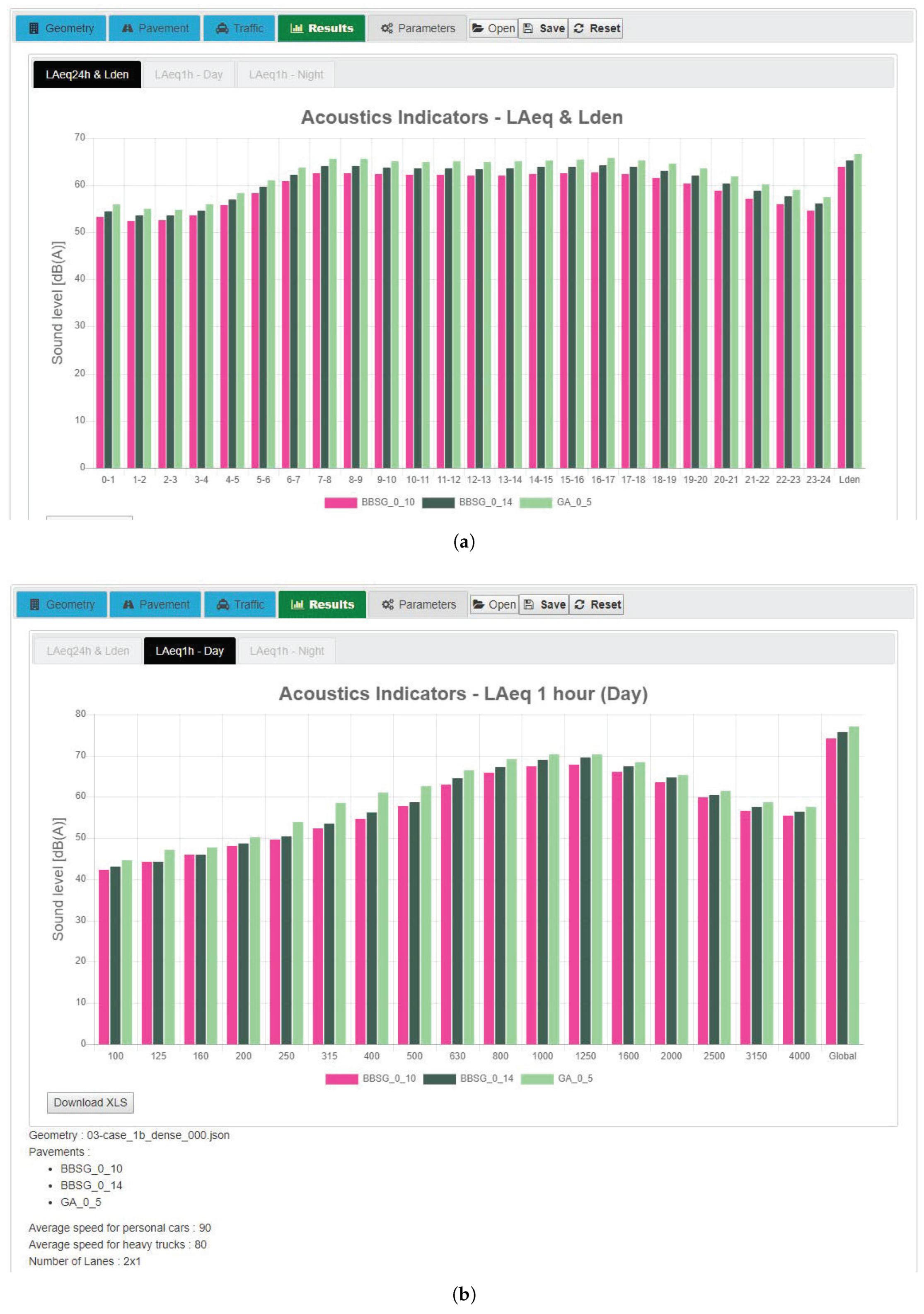
3.4. Example of DEUFRABASE Calculation

In this section, the use of the DEUFRABASE is illustrated on the basis of a realistic configuration. A ($2\times 1$) lanes road, made of a dense asphalt concrete (DAC) 0/14 pavement, was considered, with a traffic flow of 444/449 vehicles per hour for the PC on each lane (lane 1/lane 2), and 92/89 vehicles per hour for the HT. The road was bordered by grassland, creating a impedance discontinuity on the ground. The observation point was located at $7.50$ m from the right lane axis and 1.20 m above the ground, according to a CPB configuration. Thus, within the DEUFRABASE web tool (Figure 5):

• in the ‘Geometry’ tab, the configuration ‘1b, dense discontinuity, short’ is considered (see Table 1),
• in the ‘Pavement’ tab, the ‘BBSG 0/14’ pavement is selected in the database (i.e., the French name ’Béton Bitumineux Semi-Grenu (BBSG)’ of the DAC 0/14 pavement),
• in the ‘Traffic’ tab, the road traffic is distributed on both lanes, for PC and HT vehicles separately (by checking ’Your Own Traffic Data’ instead of using pre-defined data), with the reference speeds of 90 km/h and 80 km/h for the PC and HT respectively.

Finally, in the ’Results’ tab, the 24-h equivalent sound level and the day–evening–night can be displayed (Figure 5a, by considering the built-in hourly traffic distribution), as well as the 1 h equivalent sound level (Figure 5b). One of the DEUFRABASE functionalities was being able to compare several pavements for the same configuration, as illustrated at Figure 5 with two other pavements, the ’BBSG 0/10’ and the Gussasphalt (GA, German translation of ’Mastic asphalt’) ’GA 0/5’ asphalts.

In addition, because this example was based on a real configuration, one can also compared the DEUFRABASE results with the real measurements carried out for this configuration (see Section 4 for details concerning the experimental data for validation). However, because the measurements have been corrected to bring the PC speed to 100 km/h, one must also correct the DEUFRABASE results for this speed, according to the methodology proposed in the last Section 3.3.2 for the PC. In order to apply the speed correction, the DEUFRABASE results must be exported to a spreadsheet, to ‘manually’ apply Equation (19).

Table 6. Comparison of the data produced by the DEUFRABASE with measurements in the same road configuration. Since the measurements consider a PC traffic flow at 100 km/h, the DEUFRABASE results must be corrected from the reference speed of 90 km/h (ref) to 100 km/h (new).

	Measurement (${\mathit{V}}_{\mathbf{PC}}$ = 100 km/h)	DEUFRABASE Results
1/3 Octave Bands (Hz)	${\mathit{L}}_{\mathbf{Aeq}\mathbf{,}\mathbf{1}\mathbf{h}\mathbf{,}\mathbf{measure}}$ dB(A)	${\mathit{L}}_{\mathbf{Aeq}\mathbf{,}\mathbf{1}\mathbf{h}\mathbf{,}\mathbf{ref}}$ dB(A)	${\mathit{L}}_{\mathbf{Aeq}\mathbf{,}\mathbf{1}\mathbf{h}\mathbf{,}\mathbf{new}}$ dB(A)
100	48.4	43.1	43.4
125	51.5	44.2	44.4
160	52.0	46.0	46.2
200	53.8	48.6	48.8
250	57.8	50.5	50.7
315	62.4	53.5	53.6
400	62.1	56.2	56.3
500	63.2	58.8	58.9
630	67.4	64.6	64.7
800	68.3	67.2	67.3
1000	67.7	68.9	69.2
1250	68.1	69.5	69.8
1600	66.8	67.4	67.7
2000	64.7	64.7	65.0
2500	62.0	60.5	60.8
3150	60.0	57.5	57.8
4000	57.2	56.4	56.7
Global	76.2	75.7	75.9

gives the 1 h equivalent sound level obtained form the DEUFRABASE, before and after the speed correction, and shows the positive effect of the speed correction, and finally a very good agreement with the measurements (deviation is around 0.3 dB(A)).

4. Validation

Because the DEUFRABASE was based on databases and pre-calculation for specific roads configurations and propagation conditions, it seems very important to perform a large validation by comparison with in situ measurements. For this purpose, the proposed validation used measurements that have been carried out by the Ifsttar Institute (formerly LCPC) between 1990 and 1999, on 47 different road pavements, with impedance discontinuities (dense pavement/grass or porous pavement/grass), using the CPB method (7.50 m, 1.20 m). The road traffic was only composed of PC and HT, with an average speed around 100 km/h and 80 km/h respectively. For each measurement, several parameters were estimated:

• the exact number of PC and HT in each direction,
• the impedance characteristics of the different surfaces (road and close environment),
• the atmospheric conditions (temperature, wind direction and velocity),
• the vertical sound speed gradient $\partial c/\partial h$.

As detailed in

Table 7. Selected configurations for validation. Using the DEUFRABASE, several options are possible to evaluate the noise impact of a road configuration, depending on the nature of the input data. Input parameters can the one that are ‘measured’ or the one specified by the ‘database’. Speed correction, presented at Section 3.3.2, was applied on the DEUFRABASE results when necessary.

Configuration	Noise Level Results	Traffic Data	Emission Spectra	Impedance
Measurements	Measured	Measured	Measured	Measured
Prediction (worst)	DEUFRABASE	Measured	Database	Database
Prediction (intermediate)	DEUFRABASE	Measured	Measured	Database
Prediction (upper-intermediate)	DEUFRABASE	Measured	Database	Database (Similar)
Prediction (best)	DEUFRABASE	Measured	Measured	Database (Similar)

, in the framework of this validation, predictions using the DEUFRABASE can be performed in several ways:

• The a priori ‘worst’ prediction considered the real traffic data only, while the other parameters (emission spectra and impedance characteristics) can be selected in the database. In this case, all the 47 road pavements can lead to a comparison between measurements and DEUFRABASE predictions.
• The a priori ‘best’ prediction considered all real input parameters (traffic data, emission spectra and impedance characteristics). Thus, for this comparison, one must extract from the 47 road configurations, those whose impedance characteristics are ‘similar’ to the one in the DEUFRABASE. In this case, only 12 road configurations representative of the three main pavement classes (three with low noise, four with intermediate, and five noisy) can be retained. One can also consider the emission spectra given by the DEUFRABASE instead of the measured one, leading to a priori results that are a little less precise (‘upper-intermediate’).
• An ‘intermediate’ prediction was also possible, considering the real traffic data and the measured emission spectra, but using the impedance characteristics available in the DEUFRABASE. In this case, all the 47 road configurations can be considered for comparison.

The proposed validation has been performed both on spectra (Section 4.1) and $L_{\mathrm{Aeq},1\mathrm{h}}$ (Section 4.2) for various pavements and traffic conditions, and considering a speed correction for PC.

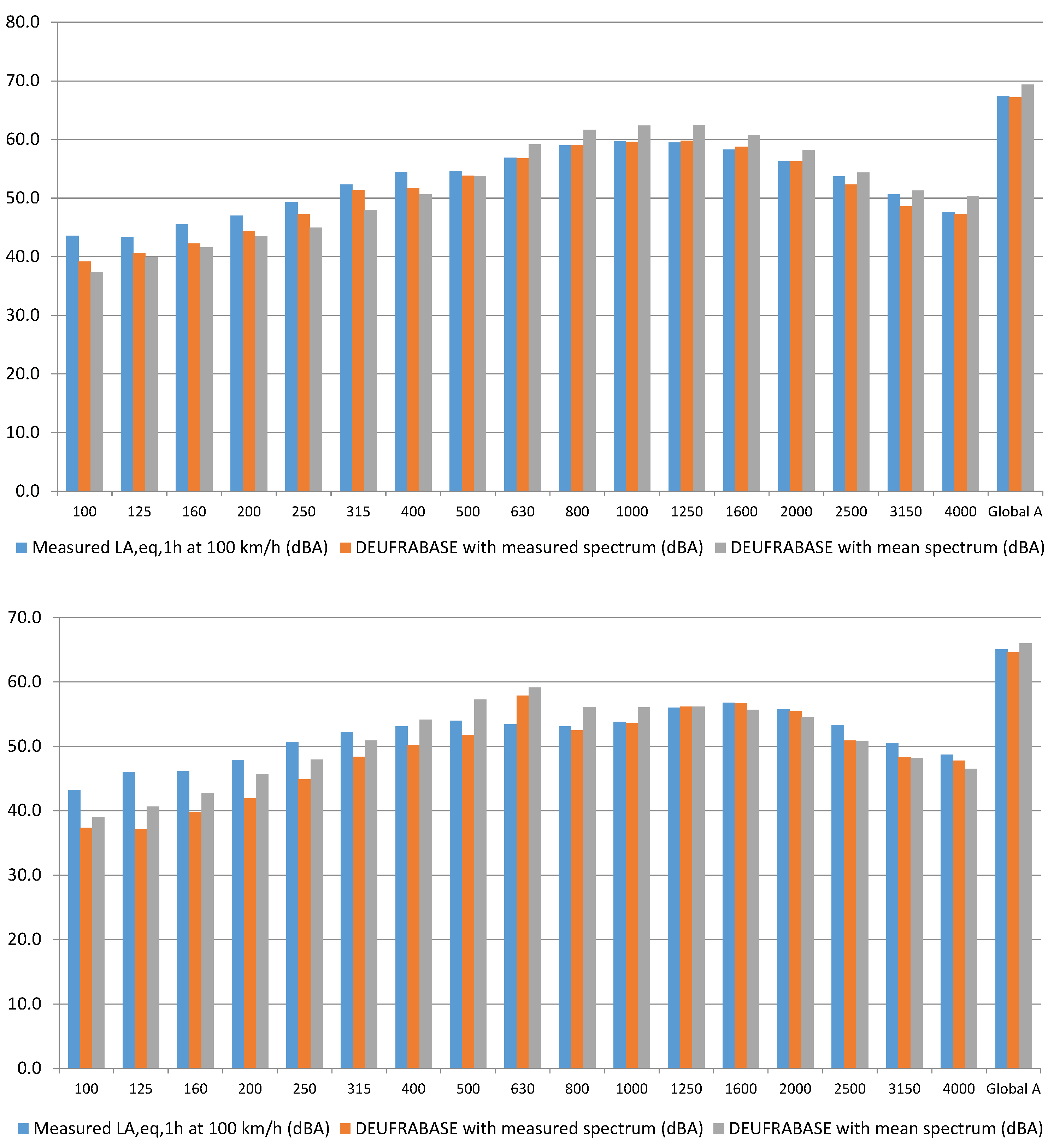
4.1. Spectral Validation

As an example, Figure 6 presents the comparison of the $L_{\mathrm{Aeq},1\mathrm{h}}$ spectrum between measurements and calculations performed with the DEUFRABASE, for a dense (DAC 0/10) pavement and for a low noise porous (PA 0/10) pavement. For the DAC 0/10, the traffic was composed of 244 vehicles with 32% of HT. For the PA 0/10, the traffic was composed of 459 vehicles with 14% of HT. In this first comparison, all the 47 road configurations are considered, using the ‘worst’ and the ‘intermediate’ DEUFRABASE predictions.

Analyzing these figures, one can conclude that:

• in global value, a very good agreement can be observed. The deviation being closed to one or two decibels;
• for each 1/3 octave band, one can note a rather good agreement between calculations and measurements above 500 Hz and particularly when considering the real measured 1/3 octave emission spectrum (red bars, ‘intermediate’ prediction) in the computation. When using an average pavement spectrum estimated from a rather large number of pavement samples for each family (gray bars, ‘worst’ prediction), which can be partially different of one particular measured pavement, the deviation is a little bit larger (around 2 dB(A)) but still acceptable. Below 500 Hz, more important differences occurred, especially for the porous asphalt. They can be explained for a small part by this difference between measured and averaged emission spectra and for a larger part by the fact that impedance values of surfaces located each side of the discontinuity, estimated from the input parameters detailed in Section 2.2.1, may slightly differ from the in situ values.

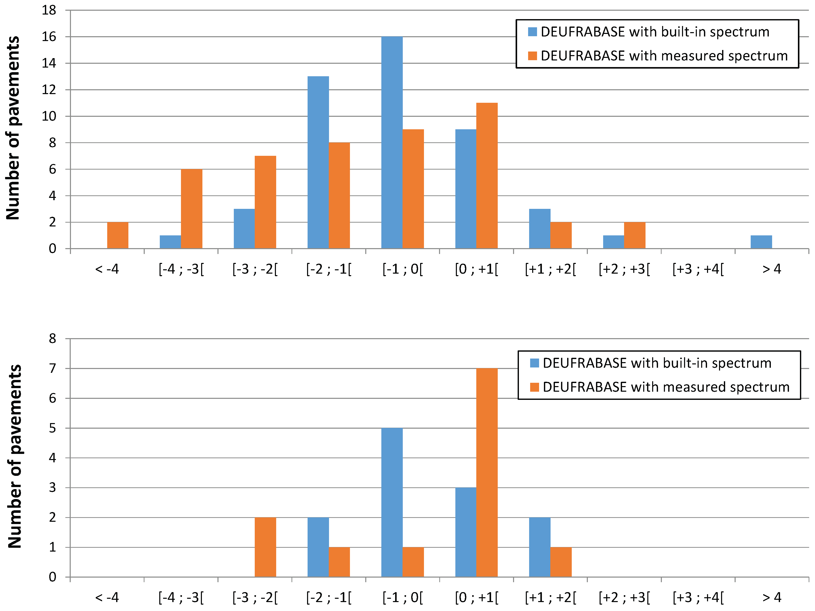
4.2. $L_{\mathrm{Aeq},1\mathrm{h}}$ Validation

Using the same approach, one can estimate the deviation between the DEUFRABASE calculations and the measured values for the $L_{\mathrm{Aeq},1\mathrm{h}}$ (in global), for all the pavements, in order to analyze the distribution of deviations. The comparison was carried out for the 47 road configurations (Figure 7, upper), considering the ‘worst’ and ‘intermediate’ predictions, and the 12 road configurations (Figure 7, lower), considering equivalent impedance characteristics (‘best’ and ‘upper-intermediate’ predictions).

Considering all the 47 road pavements (Figure 7, upper), one can observe that the deviations with the measurements are in order of ±1 dB(A) for 25/47 pavements (53%) (within ±2 dB(A) for 41/47 pavements (87%)), when using the emission spectrum from the DEUFRABASE. If the emission spectrum was the one that was measured, the deviation was around ±1 dB(A) for 42.6% of the road pavements (±2 dB(A) for 63.8%). This result shows that considering a priori better input data for the emission spectra did not increase significantly the quality of the prediction, on average.

On the other hand, when the measured impedance characteristics are as close as possible to the mean values predefined in the database (12 pavements, Figure 7, lower), the quality of prediction increases; deviations were within ±1 dB(A) for 8/12 pavements (67%) both for the measured and built-in emission spectra. One can note that, considering a deviation of ±2 dB(A), the results are better for the built-in data (100%) than for the measured spectrum (83.3%).

In conclusion, even with ‘mean values’ for the impedance and the road emission spectrum, the DEUFRABASE can predict the $L_{\mathrm{Aeq},1\mathrm{h}}$ noise level with a good accuracy as shown in the present case of 47 pavements, where 87% of comparisons are within ±2 dB(A). This result could eventually be improved if the real impedance characteristics are close enough to the predefined one, but not in significant proportions.

One can also remark that the DEUFRABASE tended to overestimate the real values (i.e., deviations are negative), which is however compatible with a usual safety margin to be taken in order to insure a better protection to the nearest residents.

5. Conclusions

In 2016, the European Commission wrote [21] that “Road traffic is the most dominant source of environmental noise in Europe. It is estimated that 125 million people are affected by noise levels from road traffic greater than 55 decibels (dB) $L_{\mathrm{den}}$, including more than 37 million exposed to noise levels above 65 dB $L_{\mathrm{den}}$”. With regard to the impact of road noise on health, reducing noise pollution is a major social issue. While solutions such as facade insulation and noise barriers help to reduce noise exposure, solutions that limit noise at the source are much more relevant. For road traffic, at suburban traffic speeds (typically above 50 km/h), rolling noise is the main source of noise pollution. Thus, in recent years, studies have focused on low noise pavements [22,23]. Generally, the acoustic characteristics of road pavements are mainly known in terms of pass-by maximum sound pressure levels $L_{\mathrm{A},\max }$ in the near field of the road or in terms of CPX index [24] in the tyre near field. Such measurements are essential but are not able to characterize the noise impact of a given pavement in the residents’vicinity. In this context, the initial goal of the present approach was to develop an operational tool to evaluate the noise impact of new (but not only) low-noise pavements, in comparison with traditional road surfaces. This tool has been implemented as a web service, called DEUFRABASE, that is freely available online [19].

The proposed approach uses two databases, the first one based on measurements of emission spectra of road vehicles on several typical pavements, and the second one made of pre-calculation of noise propagation around typical road configurations. Thus, on the basis of knowledge of the traffic flow, it allows one to obtain a fast evaluation of the noise impact of a given pavement in typical road configurations, in terms of $L_{\mathrm{Aeq}}$ (1 h or 24 h) and $L_{\mathrm{den}}$ noise levels, with a relevant accuracy.

The quality of the predictions must also be increased by considering, if available, the measured emission spectra and the details of the hourly traffic composition, instead of the pre-defined data. Considering the noise emission spectra, at this step, the tool is built from data that have been measured at reference speeds 90 and 110 km/h for passenger cars and 80 km/h for heavy trucks. Nevertheless, a speed correction is proposed in the present methodology, in order for the user to obtain an estimation of noise level indicators for other speeds. However, this speed correction is not directly implemented in the tool and requires an external processing by the user. In the future, one could proposed a built-in correction inside the tool, but also to consider noise emission spectra measured at speeds different from the reference ones. Note that the current version of the tool already allows one to upload noise emission spectra, allowing the user to test and compare their own values with the built-in data, including noise emission spectra that have been measured at specific speed.

Finally, the question of the applicability of the acoustic emission spectra of the current database, which are measured on the basis of conventional vehicles (with internal combustion engine), may legitimately arise in a context of gradual changes in the number of electric and hybrid vehicles in the road traffic flow. However, insofar as this tool focuses on assessing the noise impact of road surfaces (i.e., at suburban speeds, above 50 km/h), and because the contribution of rolling noise for new generation vehicles is equivalent to the one of more traditional vehicles [25], this database remains applicable. This is due, in particular, to the fact that the tyres that are fitted on electric/hybrid vehicles are currently identical to those fitted on traditional vehicles. However, the question may arise again when electric vehicles will use specific tyres. The DEUFRABASE can then be modified to integrate a ratio of electric/hybrid vehicles into the road traffic, as well as specific noise emission spectra.

References

1. World Health Organization. Environmental Noise Guidelines for the European Region; World Health Organization: Copenhagen, Denmark, 2018. [Google Scholar]
2. Ögren, M.; Molnár, P.; Barregard, L. Road traffic noise abatement scenarios in Gothenburg 2015–2035. Environ. Res. 2018, 164, 516–521. [Google Scholar] [CrossRef] [PubMed]
3. Directive 2002/49/EC of the European Parliament and of the Council of 25 June 2002 Relating to the Assessment and Management of Environmental Noise—Declaration by the Commission in the Conciliation Committee on the Directive Relating to the Assessment and Management of Environmental Noise. 2002. Available online: http://data.europa.eu/eli/dir/2002/49/oj/eng (accessed on 21 February 2019).
4. Kephalopoulos, S.; Paviotti, M.; Anfosso-Lédée, F. Common Noise Assessment Methods in Europe (CNOSSOS-EU); Publications Office of the European Union: Luxembourg, 2012. [Google Scholar] [CrossRef]
5. Berengier, M.; Droste, B.; Gauvreau, B.; Duhamel, D.; Auerbach, M. DEUFRABASE: A German-French acoustic database on road pavements. J. Acoust. Soc. Am. 2008, 123, 3391. [Google Scholar] [CrossRef]
6. Bérengier, M.; Pichaud, Y.; Le Fur, J.F. Effect of low noise pavements on traffic noise propagation over large distances: Influence of ground and atmospheric conditions. In Proceedings of the 29th International Congress on Noise Control Engineering, Nice, France, 27–31 August 2000. [Google Scholar]
7. International Organization for Standardization. Acoustics—Measurement of the Influence of Road Surfaces on Traffic Noise—Part 1: Statistical Pass-By Method; ISO 11819-1:1997; International Organization for Standardization: Geneva, Switzerland, 1997. [Google Scholar]
8. Bérengier, M.; Gauvreau, B.; Blanc-Benon, P.; Juvé, D. Outdoor Sound Propagation: A Short Review on Analytical and Numerical Approaches. Acta Acust. United Acust. 2003, 89, 980–991. [Google Scholar]
9. Bérengier, M.; Duhamel, D.; Gauvreau, B.; Droste, B.; Auerbach, M. A Benchmark on analytical and numerical models for road traffic noise propagation. In Proceedings of the 19th International Congress on Acoustics, Madrid, Spain, 2–7 September 2007. [Google Scholar]
10. Rasmussen, K.B. A note on the calculation of sound propagation over impedance jumps and screens. J. Sound Vib. 1982, 84, 598–602. [Google Scholar] [CrossRef]
11. Bonnet, M. Boundary Integral Equation Methods for Solids and Fluids; John Wiley: Hoboken, NJ, USA, 1999. [Google Scholar]
12. Anfosso-Lédée, F.; Dangla, P.; Bérengier, M. Sound propagation above a porous road surface with extended reaction by boundary element method. J. Acoust. Soc. Am. 2007, 122, 731–736. [Google Scholar] [CrossRef] [PubMed]
13. Lihoreau, B.; Gauvreau, B.; Bérengier, M.; Blanc-Benon, P.; Calmet, I. Outdoor sound propagation modeling in realistic environments: Application of coupled parabolic and atmospheric models. J. Acoust. Soc. Am. 2006, 120, 110–119. [Google Scholar] [CrossRef]
14. International Organization for Standardization. Acoustics—Attenuation of Sound during Propagation Outdoors—Part 1: Calculation of the Absorption of Sound by the Atmosphere; ISO 9613-1:1993; International Organization for Standardization: Geneva, Switzerland, 1993. [Google Scholar]
15. Bérengier, M.; Hamet, J. Acoustic classification of road pavements: Ranking differences due to distance from the road. Int. J. Heavy Veh. Syst. 1999, 6, 13. [Google Scholar] [CrossRef]
16. Delany, M.E.; Bazley, E.N. Acoustical properties of fibrous absorbent materials. Appl. Acoust. 1970, 3, 105–116. [Google Scholar] [CrossRef]
17. Bérengier, M.C.; Stinson, M.R.; Daigle, G.A.; Hamet, J.F. Porous road pavements: Acoustical characterization and propagation effects. J. Acoust. Soc. Am. 1997, 101, 155–162. [Google Scholar] [CrossRef]
18. Hamet, J.F.; Pallas, M.A.; Gaulin, D.; Bérengier, M. Acoustic modelling of road vehicles for traffic noise prediction: Determination of the sources heights. J. Acoust. Soc. Am. 1998, 103, 2919–2920. [Google Scholar] [CrossRef]
19. DEUFRABASE: A French-German Database for Road Noise Evaluation. Available online: http://deufrabase.ifsttar.fr/ (accessed on 21 February 2019).
20. Besnard, F.; Hamet, J.F.; Lelong, J.; Le Duc, E.; Guizard, V.; Fürst, N.; Doisy, S.; Dutilleux, G. Road Noise Prediction: 1-Calculating Sound Emission from Road Traffic; Sétra, Service d’études sur les transports, les routes et leurs aménagements: Bagneux, France, 2011. [Google Scholar]
21. Noise-Environment—European Commission. Available online: http://ec.europa.eu/environment/noise/europe_en.htm (accessed on 21 February 2019).
22. Skarabis, J.; Stöckert, U. Noise emission of concrete pavement surfaces produced by diamond grinding. J. Traffic Transp. Eng. (Engl. Ed.) 2015, 2, 81–92. [Google Scholar] [CrossRef] [Green Version]
23. Vaitkus, A.; Andriejauskas, T.; Vorobjovas, V.; Jagniatinskis, A.; Fiks, B.; Zofka, E. Asphalt wearing course optimization for road traffic noise reduction. Constr. Build. Mater. 2017, 152, 345–356. [Google Scholar] [CrossRef]
24. International Organization for Standardization. Acoustics—Measurement of the Influence of Road Surfaces on Traffic Noise—Part 2: The Close-Proximity Method; ISO 11819-2:2017; International Organization for Standardization: Geneva, Switzerland, 2017. [Google Scholar]
25. Pallas, M.A.; Bérengier, M.; Chatagnon, R.; Czuka, M.; Conter, M.; Muirhead, M. Towards a model for electric vehicle noise emission in the European prediction method CNOSSOS-EU. Appl. Acoust. 2016, 113, 89–101. [Google Scholar] [CrossRef] [Green Version]
Figure 1. General geometry of the problem: the sound source S is located at a height h S above the pavement; the reference receiver R ref is located at a height z ref above the ground and at a distance D ref from the source S (at a horizontal distance d ref from the source); the observation point R obs is located at a height z obs above the ground and at a distance D obs from the source S (at a horizontal distance d obs from the source).
Environments 06 00027 g001
Figure 2. Road geometries (see Table 1 for more details): S is the sound source (road traffic) and R the observation point. For each road configuration, the road pavement may be a dense or a porous asphalt. Note that cases (1a/1c) and (1b/1d) are the reference standardized configurations [7].
Environments 06 00027 g002
Figure 3. Average daily traffic distribution; passenger cars (PC) and heavy trucks (HT). See Table 5 for details.
Environments 06 00027 g003
Figure 4. Road configurations: ( 2 × 1 ) lanes (upper) and ( 2 × 2 ) lanes (lower). Location of the sound sources S 1 / S 2 on a 2-lanes road, and S 1 / S 2 and S 3 / S 4 on a 4-lanes road. The reference receiver is located at position R ref .
Environments 06 00027 g004
Figure 5. DEUFRABASE screenshots. Illustration of the results produced by the web tool (release V3). (a) L Aeq , 24 h and L den results. (b) L Aeq , 1 h results.
Environments 06 00027 g005
Figure 6. L Aeq , 1 h spectral comparison between DEUFRABASE calculations and measurements, in third octave band, for a dense asphalt (dense asphalt concrete (DAC) 0/10) pavement (upper) and a porous asphalt (porous asphalt (PA) 0/10) pavement (lower). DEUFRABASE predictions are based either using the mean emission spectrum (‘worst’ prediction) or using the measured spectrum (‘intermediate’ prediction).
Environments 06 00027 g006
Figure 7. Deviations from measurements, in dB(A), considering all the 47 road pavements (upper, i.e., ‘worst’ [built-in] and ‘intermediate’ [measured] predictions) and 12 ‘equivalent’ pavements (lower, i.e., ‘upper-intermediate’ [built-in] and ‘best’ [measured] predictions).
Environments 06 00027 g007