Statistical Facilitation in Environmental Science: Integrating Results from Complementary Statistical Analyses Can Improve Ecological Interpretations

Abstract

Professionals working in biological conservation seek to understand, manage, and restore populations of native organisms using many techniques. A common approach for this discipline is using long-term data collections to inform decision making. However, several quantitative issues complicate statistical analysis of monitoring datasets and can reduce the utility of results for conservation decision making. Integrating results from multiple analyses applied to the same dataset (i.e., approaching the same biological problem using different techniques) is one way to address concerns related to field data that violate statistical assumptions. This process allows data analysts, researchers, and managers to assemble insights based on the weight of evidence. Here we tested whether three different statistical techniques [(1) multiple logistic regression on original data, (2) multiple logistic regression on standardized data (i.e., mean of 0 and standard deviation of 1), and (3) random forest analysis] identified a similar hierarchy for selecting natural and anthropogenic habitat regressors. Our examination of how environmental variables affected Plains Minnow (Hybognathus placitus), a state-threatened fish, is relevant to other taxa and locations. We gained useful information from redundancies (i.e., agreements across analyses). New directions also emerged by addressing ambiguities (i.e., disagreements among results across analyses). When multiple analyses were integrated into one ecological story, a clearer interpretation emerged. Viewing different statistical tests as facilitators that provide mutual advantages can advance the understanding and application of statistical analyses applied to non-experimental field datasets.

1. Introduction

Overview. Data analysis is an essential component of environmental science, but quantitative challenges exist for conservation-related statistical analyses that use non-experimental monitoring datasets to assess the status of native and non-native organisms [1,2,3]. Biological conservation, a component of environmental science and conservation biology, is a discipline that seeks to understand, manage, and restore distributions of native organisms across state and regional spatial scales often through data-driven discovery [4,5]. However, data gaps, heterogeneity in underlying environmental conditions, violations of statistical assumptions, and other quantitative challenges can limit information gained from monitoring data collections [2,6]. Consequently, benefits to conservation that accrue from the identification of clear and actionable ecological interpretations can be limited [7,8]. Individual statistical analyses can address these quantitative challenges in different ways such that integrating results of multiple analyses undertaken on the same dataset can facilitate complementary insights. Our purpose is to illustrate the benefits of comparing and integrating outputs from three different statistical analyses that are each designed to prioritize influential environmental regressors for species distributions. We address this purpose by applying these different statistical analyses to the same dataset for the same organismal taxon to answer the same conservation question (i.e., which natural and anthropogenic habitat regressors are most useful for conservation?). We focus on the need to increase the ecological interpretation of these quantitative analyses in a way that helps on-the-ground managers make decisions [5].

Species Distribution Models. Species distribution models (SDMs) are essential statistical analyses for the quantitative assessment of plant and animal distributions [9,10]. Using classification algorithms for a binary response variable [1 (present) or 0 (absent)], SDMs can link data on locations of target taxa to multiple independent variables. The output of SDMs includes the identification of priority variables and predictions of the probability of organismal presence [11,12,13]. The extended statistical family of SDM models includes multiple logistic regression, generalized linear models, generalized additive models, classification and regression trees, random forest analysis, max-ent, and myriad other modeling options [14,15,16]. SDMs are widely used and have been developed for organisms in terrestrial [17,18], freshwater [19,20], and marine [21,22] ecosystems. The extensive peer-reviewed SDM literature includes reviews [22,23]; disciplinary syntheses [24,25]; identification of gaps in existing techniques [26,27,28]; and suggested model improvements [29,30,31]. As a substantial strength for biological conservation, SDMs often address the information needs of managers (e.g., distribution, presence, absence of taxa of interest) at the relevant spatial scales needed to make local, state, and regional management decisions. However, usefulness may be impacted by the quantitative limitations of any data analysis (e.g., sampling bias, knowledge gaps, and unsampled covariates).

Quantitative Challenges of Large-scale Monitoring Datasets. The utility of applying SDMs to biodiversity monitoring data depends on incorporating appropriate caveats that acknowledge the inevitable violations of statistical assumptions [32,33]. First, sample sizes can be limited when examining endangered, threatened, or species of greatest conservation need. For example, few available field sites may exist where these uncommon organisms are present, and rare species can require different methods of capture [34,35,36]. Second, spatial scales can affect physical and biological patterns of variability [6,37,38,39]. As a result, logistical limitations of personnel and budget can adversely affect large-scale, mixed-scale, and hierarchical sampling (i.e., we can sample often or we can sample across a broad scale, but doing both is increasingly difficult). Third, spatial scales can influence spatial heterogeneity [40,41], such that representative sampling is more difficult in large, natural systems with high habitat heterogeneity in which specific underlying conditions are often unknown [42]. Fourth, regardless of the statistical or study design and rigor of the sampling regime, some assumptions of statistical analysis (e.g., correlations among variables; irregular distributions) often remain unaddressed [7,8,43,44]. As a result of these limitations, among others, statistical results based on monitoring data can be ecologically ambiguous, inconsistent across studies, or uninterpretable, which reduces their utility for the effective conservation of environmental resources [2].

Statistical Analyses That We Compare and Integrate. Multiple logistic regression on original data, multiple logistic regression on standardized data (i.e., mean of 0 and standard deviation of 1), and random forest analysis are three different methods for analyzing species distributions that are used in biological conservation [45,46,47,48]. The underlying processes of these statistical analyses differ, but all three analyses make predictions about presence-absence outcomes and can be used to separate influential from extraneous variables. In ecology [49,50], social science [51,52,53], genetics [54], medicine [55,56], and analytics [57,58], logistic regression and random forest analyses have been compared. However, none of these comparisons have integrated the outputs of multiple analyses to show what is learned or missed by each analysis, as we do here.

Multiple Logistic Regression. Multiple logistic regression analyses on original and standardized data are established statistical analyses with well-documented foundations that have been used extensively in environmental science and resource conservation since their development over five decades ago [59,60,61]. Using the logit link function to transform observed presence-absences into odds of outcome [62,63], multiple logistic regression analysis uses binomially distributed responses to estimate unknown parameters and predict probability of outcomes [64]. Multiple logistic regression can provide reliable point estimations and related estimates of variability using maximum likelihoods for linearized data [62]. The long historical development of multiple logistic regression has led to the evolution of sophisticated procedures for model checking and diagnostics, as well as for comparisons of independent variable strength, direction, and effect size [64]. Although multiple logistic regression does not require a Gaussian (normal) distribution or homogeneity of variance (Table 1, criteria 1–2), multiple logistic regression makes assumptions about independence, linearity, measurement error, outliers, and multicollinearity (Table 1, criteria 3–7) that, if violated, can affect the accuracy of the results [64,65,66]. Nevertheless, multiple logistic regression (on original and standardized data) is a powerful, time-tested statistical analysis that has been used on a variety of taxa to address a range of biological conservation questions [67,68,69]. Multiple logistic regression has many advantages and often can be more interpretable than more complex analyses (Table 1, criteria 8–12).

Table 1. Comparison of assumptions and other considerations for multiple logistic regression and random forest analysis related to 12 criteria.

			Assumptions and Considerations
No.	Criteria		Multiple Logistic Regression		Random Forest Analysis
			Assumptions
1	Distribution		No assumption of underlying normality exists, but the dependent variable must be binary and residuals must be binomially distributed		No assumptions exist about underlying distribution including normality
2	Homogeneity of Variance		None		None
3	Independence		Data and errors are assumed to be independent (IID—identical, independently distributed). Analysts using multiple logistic regression may be able to address violations of independence by adding random effects, covariance components, and other advanced features that have been developed for multiple logistic regression		Data and errors are assumed to be independent (IID—identical, independently distributed). Flexibility in modeling approaches of random forest analysis may or may not address correlation, covariance, and interactions
4	Linearity		Multiple logistic regression assumes that there is a linear relationship between the independent variables and the log-odds (logit) of the outcome (not the outcome itself)		None. Random forest can model many types of relationships
5	Measurement Without Error		Measurement without error is an assumption of multiple logistic regression that is typically not met for field data		This is an assumption for random forest analysis, but random forest is more robust to violations of this assumption than multiple logistic regression due to bagging procedures
6	Outliers		Extreme values can alter outcomes of multiple logistic regression		Highly robust to extreme values but analysts need to check consequences of violations of this assumption
7	No Multicollinearity		Correlations among independent variables (multicollinearity) affects outcomes so analysts using multiple logistic regression must test for and avoid multicollinearity		No multicollinearity is an assumption of random forest analysis, but random forest analysis can be robust to multicollinearity (although analysts should always check to make sure there is minimal impact)
			Other Considerations
8	Overfit		Analyst’s views on this issue vary, but MLR may be less likely to overfit as variables are often selected a priori.		Analyst’s views on this issue vary, but RF may be more likely to be overfit IF the random forest model is used to determine which variables are useful
9	Parsimonious		Often a priority		Random forest analysis uses bagging and hyperparameter tuning, so parsimony is not a priority in the same way in random forest analysis as it is in multiple logistic regression
10	Metrics and Generality		Multiple evaluation metrics exist to assess generality of the analysis output (β, P, 95% CI, OR)		Creates and tests many trees so that the resulting forest is less likely to reflect non-general results
11	Prediction		Can be very effective in creating a predictive model		Often performs best for prediction
12	Ecological Interpretability		Multiple logistic regression is often easier to interpret and better informs analyst’s understanding of the relationships among independent and dependent variables		Ecological interpretation for random forest analysis varies with analyst and dataset but the output of random forest can be harder to interpret ecologically and variable behavior within the model can be opaque

Random Forest Analysis. Random forest analysis is a more recently developed statistical technique that blends linear and nonparametric approaches to predict outcomes for a single response variable using multiple independent variables. Random forest models are powerful prediction tools because model outputs are based on numerous individual trees [63,70]. Specifically, using bagging (i.e., aggregating), random forest analysis creates many regression trees for a wide range of bootstrap samples, then averages prediction, accuracy, and purity across all trees in the forest. The resulting ensemble of trees, in conjunction with the tuning of hyperparameters (regularization) for number of trees, tree depth, and variables to try per node, can reduce the likelihood of overfitting or misspecification compared with a single tree [63,71]. Random forest analysis also provides insights on variable importance and relationships among variables through partial dependency plots, receiver output characteristic curves (ROCs), and calculations of area under these curves (AUCs) [63,70]. Random forest analyses have substantial flexibility because of limited assumptions (e.g., Table 1, criteria 4–7; [49,72,73]), and are widely used in ecology [19,46,74].

Objectives. Here we address four objectives. First, we test whether three different statistical techniques identify a similar hierarchy for nine natural and anthropogenic habitat regressors. We chose these statistical analyses because multiple logistic regression on both original and standardized data [75,76,77] and random forest analyses [78,79,80] are commonly used in ecology and conservation. Second, we compare outcomes of these analyses to quantify how “redundant” results (i.e., the same outcomes in all analyses) strengthen confidence in ecological trends and how addressing and resolving “ambiguous” results (i.e., conflicting outcomes across analyses) identifies new directions. Third, we demonstrate how other types of statistical analyses (e.g., accuracy estimates, spatial prediction maps) can further inform the ecological interpretation of all statistical analyses that we examine here. Fourth, we highlight information that can be gained by integrating insights from all statistical analyses into one ecological story. In ecology, facilitation (an interaction where the presence of one entity enhances another without adverse consequences to the original entity) is increasingly viewed as a process that improves our understanding of relationships [81]. Viewing different statistical tests as facilitators that provide mutual advantages encourages data analysts to check for consistency, generality, utility, and ecological believability.

2. Materials and Methods

Study Taxon. Plains Minnow (Hybognathus placitus) is a Kansas state threatened taxon [82,83] that can serve as a general model of native prairie fish conservation. Plains Minnow presently has a much-reduced state-wide geographic range [84,85] and is currently only common in two south-central river basins in Kansas, USA (Lower Arkansas; Cimarron; [86]). Plains Minnow is a small-bodied (<127 mm maximum length), short-lived (0–2 yrs), Great Plains stream fish that consumes a generalist diet, and has early (mostly at 1 yr), infrequent reproduction (once or twice in a lifetime) [87,88]. Plains Minnow is common in medium to large rivers [89,90] and is most often associated with small substrate (e.g., sand; [91,92,93]). Plains Minnow adults spawn in the water column [92,94,95] where their semi-buoyant, non-adhesive eggs remain suspended during development [88,96]. Even though taxon-specific research on many specific anthropogenic threats is lacking, in general, native prairie fish are assumed to be adversely affected by residential and commercial development, agriculture, modification of natural systems via dams, water withdrawal, invasive species, habitat alteration, and climate change [97,98,99,100,101,102]. In Kansas, a restoration program for Plains Minnow is underway, which can benefit from foundational knowledge that will emerge from the analyses undertaken here.

Fish Data. We analyzed fish samples from the Kansas Department of Wildlife and Parks Stream Assessment and Monitoring Program database (8844 unique sample sites within all 12 major river basins). Fish data included historical specimens, ongoing fish community monitoring, and sampling from field research permits. Plains Minnow was present at 750 sample sites in this database. We transformed abundance records into presence-absence of sampled species because different methods were used across samples.

Environmental Data. We used regressors from nine ecological categories: (1) discharge, (2) substrate (% sand), (3) stream depth (m), (4) sinuosity (curviness), (5) land use, agriculture (% crop cover), (6) land use, development (%), (7) grassland (%), (8) dam characteristics (percent dam-free upstream area), and (9) gradient (m/m). Corresponding to the latitude and longitude at which fish samples were collected, we wrangled values for these physical and impact data from existing GIS datasets: (1) National Hydrography Database Plus Volume 2 [103]; (2) Soil Survey Geographic Database—SSURGO [104]; (3) National Anthropogenic Barrier Dataset—NABD [105,106]; (4) Cropscape—Cropland Data Layer (CDL), National Land Cover Database (NLCD) [107,108].

Data Cleaning. Originally, we had 750 Plains Minnow presence sites, but we removed records that had one or more missing GIS values such that a complete set of regressor data was available at 589 Plains Minnow presence sites. To avoid zero-inflation, we balanced the number of presence and absence sites by randomly removing absences to equal the number of presence sites (n = 589 Plains Minnow presence sites; 589 Plains Minnow absence sites). Predictor variables in a single model formula were not strongly correlated (Pearsons < 0.70). We used the same fish and GIS data to address the same common conservation question for each of our three statistical analyses.

Multiple Logistic Regression and Standardized Multiple Logistic Regression (Objective 1). For multiple logistic regression, we assumed a logistic distribution of errors appropriate for our presence-absence data. Parameters were estimated using a maximum likelihood function with a generalized linear model [109]. In the standardized multiple logistic regression analysis, the original regressor data were standardized to a mean of 0 and standard deviation of 1, allowing slopes (β) and odds ratios (ORs) to be compared across individual regressors.

Four evaluation criteria aided statistical and ecological interpretations of multiple regressions. For both original and standardized data, these evaluation criteria included: (1) significant p-values (≤0.05); (2) 95% confidence interval that does not include zero; (3) direction and size (standardized data only) of slope estimates (β), and (4) the size of odds ratios (ORs). A significant p-value indicated that the slope of the relationship between the probability of fish presence (Y axis) and the independent regressor (X axis) is different than zero (i.e., different from a horizontal or null relationship). A 95% confidence interval that does not include zero is a related check on whether the relationship between response and regressor differs from the null. In multiple logistic regression, the slope (β) is the change in the log-odds of the outcome (probability of presence) for a one-unit increase in the independent regressor variable. The odds ratio (OR) is the change in the odds of the outcome (presence, absence) for a one-unit increase in a predictor variable. An OR > 1 indicates that an increased likelihood of an outcome (presence) occurs with a one-unit increase in the predictor; an OR < 1 indicates a decreased likelihood of an outcome (presence) occurs with a one-unit increase in the predictor; and an OR = 1 indicates no effect of the predictor on the response.

Regression Visualizations (Objective 1). For both types of multiple logistic regression analyses, variable-specific marginal effects plots helped to visualize the relationship between the predicted probability of Plains Minnow presence (Y axis) and a specific regressor (X axis) when all other independent variables in the model were held constant. Because these plots are similar for multiple logistic regression on the original data and standardized multiple logistic regressions, only plots for the original data are shown here.

Random Forest Analyses (Objective 1). Random forest analysis is a commonly used ensemble-based classification method that is effective with large datasets [110]. Focused results can emerge when the variables for inclusion are thoughtfully chosen and hyperparameters are tuned, as performed here. The hyperparameter governing the number of subsampled predictors (mtry, randomForest package [111] was tuned using cross-validation across regressors [111,112]. Based on the results of the cross-validation, the mtry value corresponding to the lowest error rate with the least number of variables was selected [63,112]. In addition to the mtry hyperparameter, ntree (i.e., the number of individual trees in the forest) was set at the minimum number of trees to produce a stable error rate based on the visual inspection of the error rate as a function of n trees [63].

Random Forest Visualizations (Objective 1). The relative impact of individual variables in the random forest analysis was evaluated in the following two ways when the exclusion of each variable was systematically considered: (1) mean decrease in accuracy and (2) mean decrease in the Gini index [70,113]. Although less common in the literature, the Gini index explained the change in node/tree purity, which can be an impactful source of variability in the random forest analysis. Plots of both metrics provided general rankings of variable impact decreasing from right to left on the visualizations. Partial dependency plots of both raw breakpoint and LOESS-smoothed responses visualized the relationship between the predicted probability of Plains Minnow fish presence (Y axis) and the specific regressor (X axis).

Identifying Similarities and Reconciling Differences Between Analyses (Objective 2). If the three analyses differed in the prioritization of an independent variable, we evaluated four objective hypotheses to understand why these analyses that addressed similar questions differed. These hypotheses were as follows: H₁: multiple logistic regression provides inaccurate information; H₂: random forest provides inaccurate information; H₃: both analyses are incorrect; and H₄: both analyses provide useful and complementary information.

When the multiple logistic regression and random forest analyses’ outputs did not agree for a variable, we repeated each analysis with thoughtfully collected modifications of the regressor. These modifications included removing extreme points (if appropriate), applying a log transformation (if appropriate), or adding a quadratic (squared) term (if appropriate). For the original and modified variables, we compared regressor ranking, model accuracy, and shapes of the relationship between the probability of fish presence and regressor to gain more information about ambiguity across models. For brevity, we only show results of extreme value removal and quadratic transformations.

Other Complementary Analyses—Accuracy Assessment (Objective 3). Confusion matrices offer additional metrics for model accuracy (percent of true predictions in total samples). To create a confusion matrix for the multiple logistic regression model on original data, we used a 10 k-fold cross validation (caret and tidyverse, [114,115,116,117]). A confusion matrix for the random forest analysis was created post hoc using the out-of-bag error rate, i.e., the error rate of the predictions from the test datasets after being fit to the trained models [71,113]. For both analyses, receiver operating characteristic (ROC) curves, based on true and false positive rates, assisted in visualizing model performance. A ROC baseline represents no predictive power; a ROC that approaches a 100% true positive rate and 0% false positive rate identifies a better model performance.

Other Complementary Analyses—Comparing Prediction Maps (Objective 3). Maps of predictions across Kansas from both multiple logistic regression (original data) and random forest were generated using ArcGIS Pro version 3.4.3 [118]. Predictions from multiple logistic regression were stored as percentages reflecting the predicted probability of Plains Minnow presence. In contrast, predictions from random forest analysis were stored as binary classifications such that any site with greater than 50% predicted presence was classified as a 1 and any site with less than 50% predicted presence was classified as 0. These visualizations of predictions made comparisons of prioritized stream sites from analyses accessible. The different statistical approaches led to varying levels of detail (grain) in revealing the probability of presence at a given locale. The cartographic addition particularly exemplified differences and complementary views for guiding future conservation efforts while considering geographical allocation of resources.

3. Results

Multiple Logistic Regression Results (Objective 1). In the multiple logistic regression analysis on original data, five independent variables most strongly affected the probability of Plains Minnow presence. These five significant variables for which confidence intervals did not include zero were as follows: (1) stream depth, (2) percent grassland, (3) percent dam-free upstream area, (4) percent sand, and (5) gradient (Table 2). Of these, stream depth, percent grassland, percent dam-free upstream area, and percent sand had positive slopes (p ≤ 0.05; Table 2), and gradient had a significant negative slope (p ≤ 0.05; Table 2).

Table 2. Multiple logistic regression results (on original data) using the environmental regressors stream depth (estimated in meters), grassland (% in catchment), dam-free (% of upstream area free of dams), percent sand (% catchment), gradient (m/m), discharge (August, average cubic feet per second), development (% open space in catchment), crop cover (% in catchment), and sinuosity (locally averaged estimates). The response variable is probability of Plains Minnow (Hybognathus placitus) presence. Accuracy = 89%. Bolded entries with an asterisk indicate significance (p ≤ 0.05). * p ≤ 0.05 Column headings are common metrics associated with the analysis (β = parameter estimate of the slope; SE = standard error, CI = 95% confidence interval, Z = Z statistic; p = probability of a horizontal line or no effect).

			CI
Variable Name	β	SE	Lower	Upper	Z	p		Odds Ratio
(Intercept)	−9.77	2.25	−14.27	−5.45	−4.35	0.00	*	0.00
Depth	0.48	0.12	0.25	0.71	4.08	0.00	*	1.61
Grassland	0.04	0.01	0.03	0.05	7.76	0.00	*	1.04
Dam-Free	0.04	0.01	0.03	0.05	7.04	0.00	*	1.04
Sand	0.04	0.01	0.03	0.05	6.98	0.00	*	1.04
Gradient	−210.63	52.56	−321.77	−114.62	−4.01	0.00	*	0.00
Discharge	0.00	0.00	0.00	0.00	1.53	0.13		1.00
Development	−0.03	0.03	−0.10	0.03	−0.99	0.32		0.97
Crop Cover	0.00	0.01	−0.01	0.02	0.53	0.60		1.00
Sinuosity	0.03	0.07	−0.11	0.18	0.43	0.67		1.03

Standardized Logistic Regression Results (Objective 1). When regressor data were standardized, the same five regressors were significant and had 95% confidence intervals that did not cross 0 (Table 3). In addition, standardization differentiated the relative magnitude of the slopes for all five significant regressors (magnitude of β). Using the odds ratio to quantify the effect size of individual variables, increasing percent grassland, percent dam-free upstream area, percent sand, and stream depth by 1 standardized unit increased the probability of Plains Minnow presence 4.31, 3.82, 2.83, and 2.77 times, respectively (Table 3). As gradient increased by one standardized unit, the probability of Plains Minnow presence was reduced by about half (Table 3; OR = 0.48).

Table 3. Standardized multiple logistic regression results that included the following environmental regressors: grassland (% in catchment), dam-free (% of upstream area free of dams), percent sand (% catchment), stream depth (estimated in meters), gradient (m/m), discharge (August average, cubic feet per second), development (% open space in catchment), crop cover (% in catchment), and sinuosity (locally averaged estimates). The response variable is probability of Plains Minnow (Hybognathus placitus) presence. Accuracy = 89%. Bolded entries with an asterisk are significant (p ≤ 0.05). Column headings are common metrics associated with the analysis (β = parameter estimate of the slope; SE = standard error, CI = 95% confidence interval, Z = Z statistic; p = probability of a horizontal line or no effect.

			CI
Variable Name	β	SE	Lower	Upper	Z	p		Odds Ratio
(Intercept)	−0.10	0.10	−0.29	0.10	−0.95	0.34		0.91
Grassland	1.46	0.19	1.10	1.84	7.76	0.00	*	4.31
Dam-Free	1.34	0.19	0.98	1.73	7.04	0.00	*	3.82
Sand	1.04	0.15	0.75	1.34	6.98	0.00	*	2.83
Depth	1.02	0.25	0.53	1.51	4.08	0.00	*	2.77
Gradient	−0.74	0.19	−1.14	−0.40	−4.01	0.00	*	0.48
Discharge	0.26	0.17	−0.09	0.57	1.53	0.13		1.29
Development	−0.16	0.16	−0.47	0.14	−0.99	0.32		0.86
Crop Cover	0.07	0.13	−0.19	0.33	0.53	0.60		1.07
Sinuosity	0.05	0.11	−0.16	0.26	0.43	0.67		1.05

Multiple Logistic Regression—Marginal Effects Plots (Objective 1). Marginal effects visualizations reinforced the trends described above. The probability of Plains Minnow presence increased as percent grassland, percent dam-free upstream area, percent sand, and stream depth increased (Figure 1A–D). Although Plains Minnow presence was inversely associated with gradient (Figure 1E), four aspects of the gradient plot indicate that this trend merited additional scrutiny [i.e., (i) a limited data range for both X and Y axes, (ii) high variation especially at higher regressor values, (iii) several extreme values (X axis), and (iv) a very large β value]. Marginal effects plots for the variables discharge, development, crop cover, and sinuosity showed highly variable responses (Figure 1F–I).

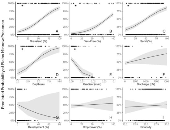
Figure 1. Marginal effects plots of environmental regressors (X axis) from top multiple logistic regression model (original data), including (A) grassland (% in catchment); (B) percent dam-free upstream area (% of upstream area free of dams), (C) percent sand (% catchment), (D) stream depth (estimated in meters), (E) gradient (m/m), (F) discharge (August average, cubic feet per second), (G) development (% open space in catchment), (H) crop cover (% in catchment), and (I) sinuosity (locally averaged estimates). The response variable is predicted probability of Plains Minnow (Hybognathus placitus) presence. An asterisk in the upper left hand corner corresponds to p-values in Table 2. Black dots are data points, the black line is the model estimate and gray shading indicates variability produced by the model from the data.

Random Forest—Variable Importance Results (Objective 1) (Table 3). Removing gradient, percent dam-free upstream area, and, to a lesser degree, percent grassland decreased the accuracy of trees in the random forest analysis, indicating that these three regressor variables strongly influenced the probability of Plains Minnow presence (Figure 2A). Removing development, crop cover, sinuosity, stream depth, percent sand, and discharge had more limited effects on accuracy (Figure 2A). Excluding gradient also decreased the Gini index, indicating that the inclusion of this regressor increased node purity and helped create a better model (Figure 2B). To a lesser degree, trees that lacked percent dam-free upstream area, and percent grassland also experienced reductions in the Gini index. Removing development, crop cover, sinuosity, stream depth, percent sand, and discharge had little impact on node purity (Figure 2B).

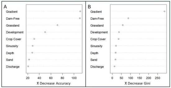
Figure 2. Variable importance of environmental regressors from a random forest analysis. Variables are ranked by (A) mean decrease in accuracy and (B) mean decrease in the Gini index. Variables include gradient (m/m), percent dam-free upstream area (% of upstream area free of dams), percent grassland (% in catchment), development (% open space in catchment), crop cover (% in catchment), sinuosity (locally averaged estimates), stream depth (estimated in meters), sand (% catchment), and discharge (August average, cubic feet per sec). Open circles show model parameter estimates.

Specific evaluation rules-of-thumb have not been developed for random forest analysis, but by combining accuracy and Gini index plots (Figure 2A,B), we can create the following hierarchy for our nine regressors (most to least impactful): gradient, percent dam-free upstream area, percent grassland, development, crop cover, sinuosity, stream depth, percent sand, discharge. Of these, gradient, percent dam-free upstream area, and percent grassland were most consistently influential in our random forest model.

Random Forest—Partial Dependency Plots (Objective 1). Partial dependency plots depicted the shape of relationships among the predicted probability of Plains Minnow presence and individual regressors for random forest analysis. LOESS-smoothed responses identified an increasing non-linear relationship between the predicted probability of Plains Minnow presence and three independent regressors (percent grassland, percent upstream dam-free area, percent sand) (Figure 3A–C, dotted line). The relationship between the predicted probability of Plains Minnow presence and stream depth was convex (Figure 3D, hump-shaped). Relationships between the predicted probability of fish presence and gradient, development, and crop cover identified inverse thresholds (Figure 3E,G,H). For variables of lesser relative impact, the probability of fish presence increased with discharge and sinuosity (Figure 3F,I).

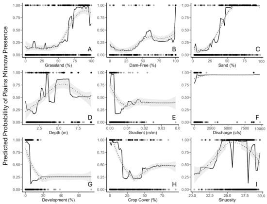
Figure 3. Partial dependency plots of predictions for environmental regressors from random forest analysis, including (A) grassland (% in catchment); (B) percent dam-free upstream area (% of upstream area free of dams); (C) percent sand (% catchment); (D) stream depth (estimated in meters); (E) gradient (m/m); (F) discharge (August average cubic feet per second), (G) development (% open space in catchment), (H) crop cover (% in catchment), and (I) sinuosity (locally averaged estimates). The response variable (Y axis) is probability of Plains Minnow (Hybognathus placitus) presence in Kansas. Black dots at the top and bottom of each plot represent presence-absence data points. Unaltered model trends are displayed by a solid black line, and LOESS-smoothed trends are shown by dotted line with model error in gray. Data correspond to Figure 2.

Identifying Similarities in the Output of the Statistical Analyses (Objective 2). The results reported above identified two useful similarities in trends across analyses. These redundancies increased confidence in our ecological interpretation of which regressors were most influential in determining Plains Minnow presence. First, for all three statistical analyses, plots agreed on the general direction of select relationships. Specifically, all analyses showed a general positive (increasing) relationship between the predicted probability of Plains Minnow presence and percent grassland, percent dam-free upstream area, percent sand, and a negative (inverse) relationship between the predicted probability of Plains Minnow presence and gradient (Figure 1A–C, Figure 2A–C and Figure 3A–C). Second, all three analyses identified the same three variables as influential (percent grassland, percent dam-free upstream area, gradient; Table 2 and Table 3; Figure 1).

Resolving Ambiguity Among Analyses to Better Understand Data Trends (Objective 2). Four ambiguities (inconsistencies) emerged across analyses. First, by providing a quantitative comparison of specific evaluation criteria (β, OR), unlike other analyses, standardized multiple logistic regression facilitated the comparison of regressor slopes (Table 2, β). For example, standardized multiple logistic regression was the only analysis to quantify that percent grassland (β = 1.46 standardized) and percent dam-free upstream area (β = 1.34 standardized) were more influential than percent sand (β = 1.04 standardized) and stream depth (β = 1.02 standardized). Multiple logistic regression on original data did not identify this distinct hierarchy that allowed effect sizes to be compared nor did random forest. Second, the impact of percent sand and stream depth differed between the multiple logistic regressions and the random forest analysis. Specifically, stream depth was significant and had high ranks (ranks 1, 4, Table 2 and Table 3) in the multiple logistic regressions, but was not highly influential in the random forest analysis (rank 7, Figure 2A,B). Similarly, percent sand was significant and had high ranks in both multiple logistic regressions (tied for rank 2, Table 2; rank 3, Table 3), but did not have a high ranking in the random forest analyses (rank 8, Figure 2). Third, the probability of Plains Minnow had a linear relationship with stream depth in the multiple logistic regressions, but had a convex (hump-shaped) relationship in the random forest analysis. Fourth, the impact of gradient differed among analyses. Specifically, gradient was the most influential regressor in the random forest analyses but was only one of five significant regressors in the two multiple logistic regressions.

Resolving Ambiguity Among Analyses—Stream Depth. Adjusting the metric used for stream depth by adding a second squared parameter (stream depth, stream depth²) increased agreement in variable impact and in the shapes of the relationship between independent and dependent variables across multiple logistic regression and random forest analyses (Figure 4A–D). Compared with the original multiple logistic regression relationship between the predicted probability of Plains Minnow presence and stream depth (Rank 4 of 9, Figure 4A), adding a squared parameter created a convex relationship between the predicted probability of Plains Minnow presence and stream depth, which increased the rank of this regressor (ranks 1, 2 of 10, Figure 4B). For the random forest analysis, quadratic parameterization of stream depth changed the shape of the relationship slightly but increased the ranks of this regressor somewhat (original: rank 8 of 9, Figure 4C; reparametrized: ranks 5–7 of 10, Figure 4D). Thus, the rank of stream depth and shape of the relationship between the probability of presence of Plains Minnow and stream depth converged between the different analyses when a squared term for stream depth was added.

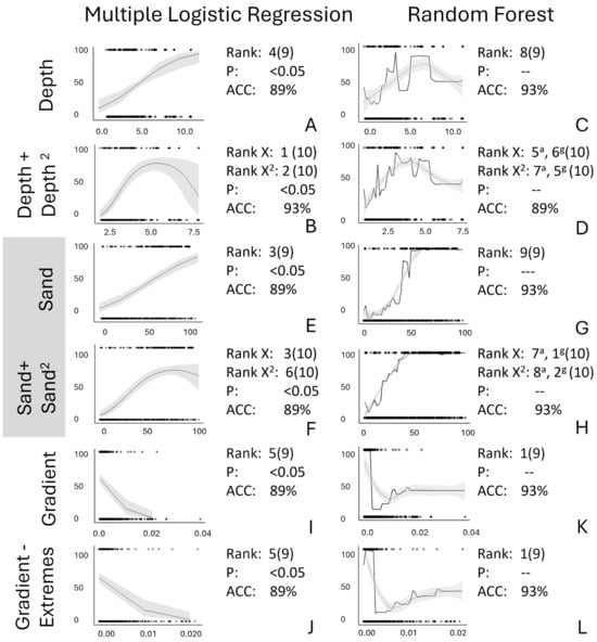
Figure 4. Relative to original model output (A,C,E,G,I,K), shown are effects of various data alterations (B,D,F,H,J,L) for partial dependency plots from multiple logistic regression (A,B,E,F,I,J) and marginal effects plots from random forest analyses (C,D,G,H,K,L). In all figures, the Y axis is probability of presence of Plains Minnow (Hybognathus placitus). On the X axis are data related to (A–D) stream depth, (E–H) percent sand, and (I–L) gradient. The rank, significant p-value for β, and accuracy (ACC) are also shown. (A,C,E,G,I,K) use original data variables. (B,D,F,H) use a quadratic transformation; (J,L) have extreme points removed. Log transformations provided little new information. In panels (D,H), the superscripts a and g indicate ranks based on both accuracy and Gini index metrics. Unaltered model trends are displayed by a solid black line, and LOESS-smoothed trends are shown by dotted line with model error shown with gray shading.

Resolving Ambiguity Among Analyses—Percent Sand. Adding a quadratic term for percent sand also explained some, but not all, discrepancies in the variable impact between multiple logistic regression and random forest (Figure 4E–H). Relative to the original linear relationship between the predicted probability of Plains Minnow presence and percent sand in the multiple logistic regression (rank 3 of 9, Figure 4E), a quadratic term added a convex threshold at extremely high values of percent sand but did not change the relative rank (ranks 3, 6 of 10, Figure 4F). For the random forest analysis, the original relationship between the predicted probability of Plains Minnow presence and percent sand (rank 9 of 9, Figure 4G) changed slightly and increased the variable ranking of some percent sand rankings when a quadratic term for percent sand was added (rankings 1, 2, 7, 8 of 10, Figure 4H). Exploration of this variable did not answer all questions about the behavior of the predicted probability of presence for Plains Minnow and percent sand, but comparing these four plots stimulated the examination of the role of non-linear relationships.

Resolving Ambiguity Among Analyses—Gradient. Adjusting the distribution of the gradient data by removing extreme points or applying a log transformation did not resolve inconsistencies between multiple logistic regression and random forest analyses (Figure 4I–L). Relative to the original multiple logistic regression model (rank 5 of 9, Figure 4I), removing extreme points from the gradient data did not increase the ranking of gradient in the multiple logistic regression or change the shape of the linear relationship between the predicted probability of fish presence and gradient (rank 5 of 9, Figure 4J). Similarly, relative to the original random forest model (rank 1 of 9, Figure 4K), removing extreme points did not change the high variable rank for gradient or alter the negative threshold curve (rank 1 of 9, Figure 4L).

Other Analyses That Complement All Analyses Tested—Accuracy (Objective 3). Both models had high prediction accuracy (Figure 5). Our multiple logistic regression model generated 89% accuracy and 90% precision (Figure 5A); our random forest analysis had 93% accuracy and 91% precision (Figure 5B). Both models predicted fewer false presences than absences. The random forest model (Figure 5B) produced fewer misclassified observations overall than multiple logistic regression (Figure 5A). ROC curves from both models performed with a predictive power substantially higher than the baseline (Figure 5C,D), but the random forest model had a slightly greater area under the curve (Figure 5D) than the multiple logistic regression (Figure 5C). Confusion matrices helped interpret each analysis and facilitated a useful comparison across analyses.

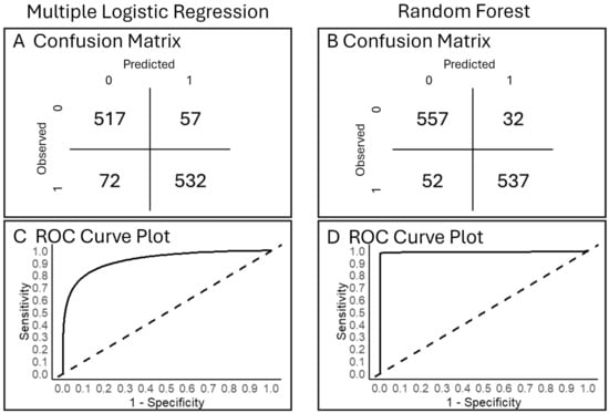
Figure 5. For (A,C) multiple logistic regression and (B,D) random forest models for probability of Plains Minnow presence, shown are (A,B) confusion matrices. (C,D) Receiver operating characteristic (ROC) curves. In (C,D), solid lines show the tradeoff between true positive rate and false positive rate across all possible classification probability thresholds; the dotted lines are the expected null specificity/sensitivity. The space above and to the left of the dotted line indicates better model performance than the null.

Other Analyses That Complement All Analyses Tested—Spatial Prediction Maps (Objective 3). Model prediction maps differed between statistical analyses in a way that showed additional unique advantages of each approach (Figure 6) and the benefits of integrating both analyses. The spatial presentation of multiple logistic regression predictions showed a state-wide gradient of low to high likelihood of Plains Minnow presence (Figure 6A). For example, sites with 88–100% predicted probability of presence occurred along the northeast border of Kansas in the Missouri River and in southern Kansas within the Lower Arkansas and Cimmaron river basins. Random forest analysis predictions were presented with binary symbology to reflect the prediction cutoffs as opposed to a gradient (Figure 6B). Most sites for which the random forest model predicted the presence of Plains Minnow occurred in the Lower Arkansas and Cimmaron river basins. Presence-absence maps from the random forest model gave easy-to-process guidance and may be better suited for quick decision making. Multiple logistic regression prediction maps identified a wider gradation of promising stream sites that can drive thoughtful in-depth discussions of locations on which to focus for sampling or restoration. Agreement in likelihood of fish presence in a region or at particular sites increases confidence in allocating resources for sampling, while disagreements may highlight a loss of historical populations due to habitat degradation and possible needs for restoration. Interpreting prediction maps from both analyses together can provide even more utility than using either approach alone.

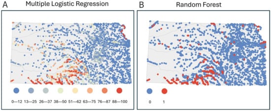
Figure 6. Modeled spatial predictions of probability of Plains Minnow presence based on (A) multiple logistic regression and (B) random forest analysis. Dot colors indicate probability of Plains Minnow (Hybognathus placitus) presence.

4. Discussion

Take Home Message 1—Strengths of Each Analysis (Objective 1): Multiple Logistic Regression. A major strength of multiple logistic regression (both on original and standardized data) is the existence of a suite of quantitative evaluation metrics for each regressor (P, 95% CI, β direction—magnitude, OR [119,120]). Each evaluation metric has an associated rule-of-thumb, based on supporting evidence, that guides the interpretation of the statistic. As a result, multiple researchers and managers can consistently form a shared consensus about relative variable impact using these rules-of-thumb for evaluation criteria. The resulting variable hierarchy can be either categorical (significant or not significant) or regressor rankings (1, 2, 3). In both of our multiple logistic regression analyses, all evaluation metrics provided consistent ecological information about the most influential regressors, which allowed us to construct a categorical hierarchy (i.e., significant: percent grassland, percent dam-free upstream area, stream depth, percent sand, gradient; non-significant: all others).

A related strength for multiple logistic regression is that, because of these agreed-upon rules-of-thumb for multiple evaluation metrics, underlying relationships can be easier to interpret in multiple logistic regression than in more complex analyses [49,53]. In particular, the relative variable impact of ecological variables can assist researcher-manager teams to prioritize future field studies and relevant monitoring collections by proposing key relationships and allocating limited resources. Furthermore, the estimates and confidence intervals from unstandardized multiple logistic regression processes offer the benefit of direct ecological translation through retaining real-world units of measurement for each environmental variable. The easy-to-understand output from this form of the model creates advantages for proposing management action and conserving key habitat conditions.

Strengths of Each Analysis (Objective 1): Random Forest Analysis. Random forest analysis also has substantial strengths for predicting ecological distributions. First, random forest compiles predictions from many trees, which makes the statistical procedure more robust to deviations in statistical assumptions than multiple logistic regression. Although our accuracy statistics were similarly high across analyses, elsewhere random forest analysis can provide higher accuracy [50,52,55,57]. Second, random forest analysis provides two metrics to evaluate relative variable impact: an accuracy metric and the Gini index (number of data points that belong to a single class at a given node). The random forest goal of achieving maximum purity (i.e., highest percentage of a single class relative to all classes) at a given node (i.e., a split or decision point) from the root (i.e., the starting point or the entire dataset) to the terminal node (i.e., leaf node or final decision) provides useful information on the data quality. In our random forest analysis, these two metrics supported the conclusion that specific individual regressors (gradient, percent dam-free upstream area, and to a lesser extent percent grassland) strongly influenced the predicted probability of Plains Minnow presence. Third, random forest analysis is more flexible in modeling trends compared with multiple logistic regression. For example, random forest analysis can model non-linear trends [63]. This flexibility provided substantial advantages for understanding the roles of percent depth and percent sand on Plains Minnow distribution.

Take Home Message 2—Weaknesses of Each Analysis (Objective 1): Multiple Logistic Regression. Multiple logistic regression analysis (on original and standardized data) has strengths but also offers some concerns that need careful consideration in statistical and ecological interpretation [65,120,121,122]. First, p-values are approximations and can be influenced by non-normal variable distributions and outliers. Exact p-values are unreliable with field data, but general p-values, as we present here, helped us prioritize regressors to consider first [123]. Second, multiple logistic regression can only detect select trends because this analysis assumes linearity of independent variables and log-odds of the dependent variable [64,65,66]. In our results, we observed that non-linear relationships for percent sand and stream depth could only be addressed in multiple logistic regression by transformation or parametrization prior to model fitting, which is inherently handled by default in random forest. Third, multiple logistic regression is sensitive to violations of many statistical assumptions (Table 1; criteria 4–7; [119,121,124]).

Weaknesses of Each Approach (Objective 1): Random Forest. Random forest analysis also has concerns that require careful consideration in statistical and ecological interpretation [125,126]. First, we found that random forest currently lacks quantitative rules-of-thumb to help analysts interpret a commonly agreed-upon set of regressor priorities. This makes ecological interpretations of variable impact more subjective. For example, does the intermediate accuracy value for percent development indicate that this regressor is worthy of additional examination or not (Figure 2A)? Does the intermediate Gini index for percent dam-free upstream area and percent grassland indicate that a concern exists with the purity of the summary tree or not (Figure 2B)? Second, we found, as have others, that understanding how variables and variable relationships contribute to predictions can be difficult because of the model complexity [126]. Hence, ground truthing the model to assess whether underlying relationships make ecological sense is often not possible. Meaningful application to conservation can be ineffective when data analysts cannot explain the underlying drivers of trends to managers and the public. Third, we found that influential points in non-linear trends identified by random forest analysis need to be interpreted carefully and verified empirically. Peaks, valleys, and thresholds that create non-linear relationships can change dramatically with small changes in the data or with different modeling tools/programs.

Take Home Message 3—Redundancies are Useful (Objective 2). We gained useful information about where and why target fish were present or absent by examining redundancies that emerged when multiple analyses agreed about specific variables. All three analyses identified percent grassland, percent dam-free upstream area, and gradient as influential. Similarly, all three analyses identified consistent directions in the relationships between the probability of Plains Minnow presence with gradient (negative), percent grassland (positive), percent dam-free upstream area (positive), and percent sand (positive). These points of agreement across analyses increased our confidence in the statistical and ecological interpretations of relationships. As an ecological benefit, our researcher-manager team gained useful information for the habitat associations of and threats to Plains Minnow, from which further conservation research and species protection policies can develop. Especially when gaps exist in large datasets, redundancy across analyses provides a strong foundation on which to build.

Take Home Message 4—Ambiguities Across Analyses Can Guide Future Directions (Objective 2). New directions emerged by addressing ambiguities upon which analyses did not agree (Table 2 and Table 3 vs. Figure 2; Figure 1 vs. Figure 3). Substantial differences between multiple logistic regression and random forest existed for the variable impact of stream depth and percent sand. Multiple linear regression identified these variables as influential (p ≤ 0.05, confidence intervals that do not include zero), whereas random forest did not rank these regressors high based on accuracy or node purity. Furthermore, the shape of response trends for these two variables differed across analyses in that random forest predicted non-linear responses and multiple logistic regression did not. These inconsistencies forced us to re-examine stream depth and percent sand. In so doing, we discovered that a quadratic function increased convergence in relationship shape and rank among analyses for stream depth, and a non-linear relationship may improve fit and convergence for percent sand. This hump-shaped response indicates that whether the regressor has a positive or negative relationship with fish presence depends on the position of the X value relative to the Y maximum. Thus, ecologically, we learned that particular ranges of conditions may be highly influential for understanding regressor–fish relationships (e.g., thresholds, peaks, and valleys).

Ambiguities in how multiple logistic regression and random forest evaluated gradient provided a different lesson. Removing extreme points or applying transformations to the gradient dataset intensified rather than reduced the differences in variable impact between multiple logistic regression and the random forest analysis. Although we could not get relationships and ranks for gradient to agree across analyses, this ambiguity forced us to scrutinize the underlying data from an ecological perspective. Kansas is a relatively low gradient state [127]. Although an east-to-west elevation gradient exists (200–1200 m), the eastern and central regions of the state where most wetted streams occur are less variable (200–600 m; [128]). Thus, differences between high and low gradient stream sites in Kansas are small. Because the hotspot of current Plains Minnow populations in south-central Kansas has a non-representative gradient distribution, this variable likely represents a statistically significant but ecologically irrelevant trend.

Across all ambiguities, disagreement among models often highlighted a need for reformulating variables to capture non-linear relationships. Comparing changes in model outputs after thoughtfully adjusting data (via changes in distributional characteristics or using different variable transformations) may (stream depth, partial—percent sand) or may not (gradient, partial—percent sand) align the outputs of different statistical analyses. The presence of two parameters that need to be interpreted together (X, X²) can add to the complexity of understanding regressors that are represented by quadratic relationships (i.e., stream depth, percent sand). For all ambiguities, comparing responses across statistical models provided useful statistical and ecological information about variable behavior and showed that the different analyses complemented each other (Objective 2, H₄).

Addressing Assumptions and Other Considerations. Field data will never meet all statistical assumptions. Thus, any statistical analysis of monitoring data needs to explicitly and realistically assess the impact of the unavoidable violation of statistical assumptions. If too many assumptions are violated, statistical outcomes may be adversely affected. Some criteria, such as the lack of assumptions about the normality of the underlying distribution or homogeneity of variance, are benefits for all analyses we examined (Table 1, criteria 1, 2). All analyses, including those we compared here, require data points to be independent unless strictly accounted for, which further complicates ecological interpretation (Table 1, criterion 3; [63,124,129]). Some criteria provide advantages for random forest. For random forest, no assumption exists about linearity, but in multiple logistic regression, the log-odds transformation of the dependent variable is assumed to be a linear function of the independent variables (Table 1, criterion 4; [63,65]). As another advantage, random forest makes limited assumptions related to measurement error, outliers, and multicollinearity (Table 1, criteria 5–7; [126,129,130]). Some considerations provide advantages for multiple logistic regression. For example, multiple logistic regression may be less likely to overfit models because a parsimonious approach is often favored (Table 1, criteria 8–9; [65,112,119,120,121,122,124,126,129,130]). Some criteria, such as the need for high quantities of data, can be disadvantages for both analyses [125]. Some considerations can be either advantages or disadvantages depending on the overarching question addressed and whether the analysis is used solely for prediction or for both understanding and prediction (Table 1, criteria 10–12; [131,132]). Problematic violations of statistical assumptions potentially can be identified in exploratory plots such that extreme points that cause problems can be removed and useful transformations can be applied prior to data analysis. Realistically, however, for analyses that use large monitoring datasets, a large number of data conditions could violate assumptions of statistical analyses, and these potential violations may or may not change the outcomes of analyses. For this reason, we propose that an across-analysis comparison, as we identify here, can serve as a practical post-analysis check for issues that may have been overlooked or which were not initially considered to be problematic.

In summary, we conclude that, although restricted by many assumptions (Table 1, criteria 4–7), the output of multiple logistic regression may be more focused and interpretable because of clear evaluation metrics (Table 1, criteria 10, 12). On the other hand, random forest can model a wider variety of relationships (Table 1, criterion 4), be more robust to underlying data issues (Table 1, criteria 5–7), and be a superior prediction tool (Table 1, criterion 11; [49]), but also can produce complex outcomes that make understanding mechanisms underlying predictions difficult to interpret (Table 1; criterion 12). The process that we describe here for comparing the output of multiple tools is one way to ground truth the consequences (insignificant to severe) of potential violated assumptions.

What We Learned From Comparing Then Integrating Multiple Analyses (Objective 4). Our approach demonstrated several ways that useful information can be gained if multiple analyses are integrated into one ecological story rather than considering each individual analysis as a stand-alone snapshot of a complex and uncertain reality. First, redundancy (i.e., repeating the same ecological question with a different statistical technique) can erroneously be viewed as a waste of effort, but redundancy in results across similar analyses enhanced our confidence that percent grassland and percent dam-free upstream area consistently and strongly influenced the presence of Plains Minnow. From this, we can prioritize with our agency partners future research and management to protect and mitigate impacts on the species’ native prairie stream habitat. Second, exploring ambiguities (i.e., competing answers provided by different analyses) is often not valued, because clear answers are preferred in research, management, grant review, and journal article publication. However, exploring ambiguities that emerged across analyses provided useful insights. For example, we learned that the relationships between the presence of Plains Minnow and stream depth and percent sand were likely non-linear. Examining ambiguities also revealed that gradient was probably ecologically irrelevant regardless of why analyses disagreed. Examining ambiguities, especially in non-linear trends, can guide future activities such as identifying specific values for environmental conditions to sample in future empirical studies (e.g., location and magnitude of peaks, valleys, inflection points, and thresholds for non-linear variables). Redundancies and ambiguities would not have been identified if we had not compared results across analyses.

Ecological Insights Gained About the Plains Minnow. Peer-reviewed field studies on the ecology of Plains Minnow in the United States Great Plains are limited [85,133,134,135,136,137,138,139]. Many existing studies of Plains Minnow in the United States Great Plains confirm the adverse effect of dams [85,133,135,138,139]. However, much of the existing United States Great Plains literature on Plains Minnow does not assess the role of the widely available natural and anthropogenic habitat variables that we examined here (e.g., depth, sinuosity, land type, gradient, whole drainage flow).

Many of the existing peer-reviewed studies on Plains Minnow focus on adverse and unnatural flow patterns, water withdrawals, and flow fragmentation related to poor water management practices [85,134,135,137,138,139,140,141]. These studies using site-specific flow data unquestionably add to our knowledge base. However, flow data used in these studies are often either (a) not from the specific times and places at which fish were sampled (i.e., limited to or extrapolated from stream gages at a few specific sites) or (b) are not available for the times and places that most fish are surveyed (i.e., site specific flow data are not generalizable to new locations and a broader scale). For example, widely available flow data such as that from NHDPlus estimate discharge or velocity in the entire catchment above a sample site and are useful for hydrological models but not for describing the flow conditions that fish experience at specific sites. Thus, regardless of the analysis tool used, a mismatch often exists for Plains Minnow and other prairie stream fish studies between fish-relevant, site-specific flow data and the state-wide scale at which conservation decisions are required.

Our Primary Take-Away and Recommendation. For field data that often violate assumptions of common statistics, our data strongly support our primary take-away that a single statistical analysis alone does not provide the ecological insights needed to plan future research or execute specific management actions. It is the integration of results from multiple analyses on the same dataset that identified accumulated points of agreement on which to build (redundancies) and future data needs (directions that emerge from addressing ambiguities). Our study showed a detailed comparison of common analysis tools applied to an extensive state survey dataset. Our most useful insights address consistency and inconsistency among analyses. As such, we propose that our process for evidence-driven assessment of strengths and weaknesses is useful for many species analyses for which survey data are available.

What is Needed: Realistic Expectations. We hope our paper serves as a reminder about the goals, achievements, and challenges of data-driven environmental field studies. At best, a single field research study contributes limited answers about the complexity and dynamism that natural systems exhibit. For most natural systems, we do not know the “true” underlying processes that drive a system or have “correct” estimates of relevant parameters for populations and communities. Thus, realistically we cannot assess whether we are “right or wrong” in the conclusions that we draw in a single study. All members of the environmental profession could benefit from merging our current rigorous quantitative quest for evidence-based understanding of natural systems through data collection analysis with more realistic expectations that also emphasize what is not yet known. This more realistic set of expectations will still celebrate the new insights that are identified from specific research and management datasets but will also provide a broader context that stresses gaps and clarifies constraints in interpretation. As a result, the combined body of relevant environmental field studies can better guide connected future activities that accumulate knowledge.

What Is Needed: Successful Disciplinary Interpretation of Statistical Patterns. The discipline of applied statistics provides tools to help environmental scientists understand natural and disturbed environmental patterns, but simply using these tools on environmental data is not a useful conservation endpoint. Thus, interpretation of the ecological meaning of complex statistics should be an overarching goal of applied statistical analysis. At present, a structured pathway to turn statistical results into disciplinary understanding is poorly defined. In many university training programs, emerging professionals become skilled at running and reporting output from sophisticated statistical analyses. Interpreting what complex analyses mean for individual disciplines, like ecology, is often missing from our current professional toolbox. Without clear pathways for interpretation that identify both advances and caveats, applying our analytical skills to practical targets such as watershed management and species protection policies will be difficult. Showing where the analyses agree (redundancies) and where biologists should be skeptical about trends (ambiguities) is a first step in developing this practical roadmap for ecological interpretation.

5. Conclusions

Our one-story approach builds on the strength of each analysis while minimizing their weaknesses. As one example, strengths of multiple logistic regression (i.e., multiple evaluation metrics with evidence-based rules-of-thumb that can make ecological interpretation more generalizable and straightforward) counterbalance a weakness of random forest (i.e., subjective metric evaluation criteria and complex underlying relationships that can make models hard to interpret and ground truth). As a second example, a strength of random forest (i.e., a sophisticated underlying algorithm allows the modeling of linear and non-linear relationships with few assumptions) offsets a weakness of multiple logistic regression (i.e., a high number of restrictive assumptions that prevent direct modeling of non-linear relationships). Thus, one way to test the rigor and relevance of results for the analysis of natural field data, which often violate statistical assumptions, is to compare and integrate the ecological interpretations of multiple analyses, as we do here. Utilizing insights from multiple analyses to create one ecological story enhances the value of take-homes compared with either analysis alone.

References

- Bolker, B.M.; Brooks, M.E.; Clark, C.J.; Geange, S.W.; Poulsen, J.R.; Stevens, M.H.H.; White, J.S.S. Generalized linear mixed models: A practical guide for ecology and evolution. Trends Ecol. Evol. 2009, 24, 127–135. [Google Scholar] [CrossRef]
- Lindenmayer, D.B.; Likens, G.E. Adaptive monitoring: A new paradigm for long-term research and monitoring. Trends Ecol. Evol. 2009, 24, 482–486. [Google Scholar] [CrossRef] [PubMed]
- Counihan, T.D.; Bouska, K.L.; Brewer, S.K.; Jacobson, R.B.; Casper, A.F.; Chapman, C.G.; Waite, I.R.; Sheehan, K.R.; Pyron, M.; Irwin, R.E.R.; et al. Identifying monitoring information needs that support the management of fish in large rivers. PLoS ONE 2022, 17, e0267113. [Google Scholar] [CrossRef] [PubMed]
- Soulé, M. What is conservation biology? Ceylon J. Sci. Biol. Sci. 1985, 35, 727–734. [Google Scholar]
- Robinson, J.G. Conservation biology and real-world conservation. Conserv. Biol. 2006, 20, 658–669. [Google Scholar] [CrossRef]
- Bisson, P.; Hillman, T.; Beechie, T.; Pess, G. Managing expectations from intensively monitored watershed studies. Fisheries 2024, 49, 8–15. [Google Scholar] [CrossRef]
- Olsen, A.R.; Sedransk, J.; Edwards, D.; Gotway, C.A.; Liggett, W.; Rathbun, S.; Reckhow, K.H.; Yyoung, L.J. Statistical issues for monitoring ecological and natural resources in the United States. Environ. Monit. Assess. 1999, 54, 1–45. [Google Scholar] [CrossRef]
- Biber, E. The challenge of collecting and using environmental monitoring data. Ecol. Soc. 2013, 18, 14. [Google Scholar] [CrossRef]
- Guisan, A.; Thuiller, W. Predicting species distribution: Offering more than simple habitat models. Ecol. Lett. 2005, 8, 993–1009. [Google Scholar] [CrossRef]
- Guillera-Arroita, G.; Lahoz-Monfort, J.J.; Elith, J.; Gordon, A.; Kujala, H.; Lentini, P.E.; McCarthy, M.A.; Tingley, R.; Wintle, B.A. Is my species distribution model fit for purpose? Matching data and models to applications. Glob. Ecol. Biogeogr. 2015, 24, 276–292. [Google Scholar] [CrossRef]
- Elith, J.; Leathwick, J.R. Species distribution models: Ecological explanation and prediction across space and time. Annu. Rev. Ecol. Evol. Syst. 2009, 40, 677–697. [Google Scholar] [CrossRef]
- Dormann, C.F.; Schymanski, S.J.; Cabral, J.; Chuine, I.; Graham, C.; Hartig, F.; Kearney, M.; Morin, X.; Römermann, C.; Schröder, B.; et al. Correlation and process in species distribution models: Bridging a dichotomy. J. Biogeogr. 2012, 39, 2119–2131. [Google Scholar] [CrossRef]
- Vasconcelos, R.N.; Cantillo-Pérez, T.; Franca Rocha, W.J.S.; Aguiar, W.M.; Mendes, D.T.; de Jesus, T.B.; de Santana, C.O.; de Santana, M.M.M.; Oliveira, R.P. Advances and challenges in species ecological niche modeling: A mixed review. Earth 2024, 5, 963–989. [Google Scholar] [CrossRef]
- Gastón, A.; García-Viñas, J.I. Modelling species distributions with penalised logistic regressions: A comparison with maximum entropy models. Ecol. Model. 2011, 222, 2037–2041. [Google Scholar] [CrossRef]
- Valavi, R.; Elith, J.; Lahoz-Monfort, J.; Guillera-Arroita, G. Flexible species distribution modelling methods perform well on spatially separated testing data. Glob. Ecol. Biogeogr. 2023, 32, 369–383. [Google Scholar] [CrossRef]
- Ramampiandra, E.C.; Scheidegger, A.; Wydler, J.; Schuwirth, N. A comparison of machine learning and statis-tical species distribution models: Quantifying overfitting supports model interpretation. Ecol. Model. 2023, 481, 110353. [Google Scholar] [CrossRef]
- Chen, J.; Zhang, Z.; Yu, M.; Su, Y.; Dai, R.; Zhan, M.; Zhang, X.; Xu, H.; Wei, Q.; Fan, W.; et al. Multidimensional niche advantages reveal how the red fox stands out in mesopredator release within terrestrial island habitats. Glob. Ecol. Conserv. 2025, 62, e03714. [Google Scholar] [CrossRef]
- Braham, M.A.; Brandes, D.; Poessel, S.A.; Duerr, A.E.; Miller, T.A.; Sur, M.; Hall, J.C.; Brandt, J.; Uyeda, L.; Astell, M.; et al. Aeroecology drives seasonal movements and predicts future distributions of a critically endangered terrestrial bird. Curr. Biol. 2025, 35, 3750–3758.e5. [Google Scholar] [CrossRef]
- Talarico, L.; Catucci, E.; Martinoli, M.; Scardi, M.; Tancioni, L. Modelling Salmo trutta complex spatial distribution in central Italy: A random forest approach revealing underrepresented lowland populations based on spatial-ly-explicit predictors. Ecol. Evol. 2025, 15, e71658. [Google Scholar] [CrossRef]
- Nguyen, B.D.; Messick, J.; Rodger, A.W.; Jackson, V.; Butler, C.; Taylor, A.T. Lumping and splitting of distribution models across a biogeographic divide informs the conservation of an imperiled fluvial fish. Ecol. Evol. 2025, 15, e71315. [Google Scholar] [CrossRef]
- Robinson, L.M.; Elith, J.; Hobday, A.J.; Pearson, R.G.; Kendall, B.E.; Possingham, H.P.; Richardson, A.J. Pushing the limits in marine species distribution modelling: Lessons from the land present challenges and opportunities. Glob. Ecol. Biogeogr. 2011, 20, 789–802. [Google Scholar] [CrossRef]
- Melo-Merino, S.M.; Reyes-Bonilla, H.; Lira-Noriega, A. Ecological niche models and species distribution models in marine environments: A literature review and spatial analysis of evidence. Ecol. Model. 2020, 415, 108837. [Google Scholar] [CrossRef]
- Frans, V.F.; Liu, J. Gaps and opportunities in modelling human influence on species distributions in the An-thropocene. Nat. Ecol. Evol. 2004, 8, 1365–1377. [Google Scholar] [CrossRef] [PubMed]
- Austin, M. Species distribution models and ecological theory: A critical assessment and some possible new approaches. Ecol. Model. 2007, 200, 1–19. [Google Scholar] [CrossRef]
- Wisz, M.S.; Pottier, J.; Kissling, W.D.; Pellissier, L.; Lenoir, J.; Damgaard, C.F.; Dormann, C.F.; Forchhammer, M.C.; Grytnes, J.-A.; Guisan, A.; et al. The role of biotic interactions in shaping distributions and realised assemblages of species: Implications for species distribution modelling. Biol. Rev. 2013, 88, 15–30. [Google Scholar] [CrossRef]
- Elith, J.; Graham, C.H. Do they? How do they? WHY do they differ? On finding reasons for differing performances of species distribution models. Ecography 2009, 32, 66–77. [Google Scholar] [CrossRef]
- Buckley, L.B.; Urban, M.C.; Angilletta, M.J.; Crozier, L.G.; Rissler, L.J.; Sears, M.W. Can mechanism inform species’ distribution models? Ecol. Lett. 2010, 13, 1041–1054. [Google Scholar] [CrossRef]
- Yates, K.L.; Bouchet, P.J.; Caley, M.J.; Mengersen, K.; Randin, C.F.; Parnell, S.; Fielding, A.H.; Bamford, A.J.; Ban, S.; Barbosa, A.M. Outstanding challenges in the transferability of ecological models. Trends Ecol. Evol. 2018, 23, 790–802. [Google Scholar] [CrossRef]
- Meynard, C.N.; Leroy, B.; Kaplan, D.M. Testing methods in species distribution modelling using virtual spe-cies: What have we learnt and what are we missing? Ecography 2019, 42, 2021–2036. [Google Scholar] [CrossRef]
- Zurell, D.; Franklin, J.; König, C.; Bouchet, P.J.; Dormann, C.F.; Elith, J.; Fandos, G.; Feng, X.; Guillera-Arroita, G.; Guisan, A.; et al. A standard protocol for reporting species distribution models. Ecography 2020, 43, 1261–1277. [Google Scholar] [CrossRef]
- Sharma, S.; Winner, K.; Pollock, L.J.; Thorson, J.T.; Mäkinen, J.; Merow, C.; Pedersen, E.J.; Chefira, K.F.; Portmann, J.M.; Iannarilli, F.; et al. No species left behind: Borrowing strength to map data-deficient species. Trends Ecol. Evol. 2025, 40, 699–711. [Google Scholar] [CrossRef]
- Jarnevich, C.S.; Stohlgren, T.J.; Kumar, S.; Morisette, J.T.; Holcombe, T.R. Caveats for correlative species distribution modeling. Ecol. Inform. 2015, 29, 6–15. [Google Scholar] [CrossRef]
- Webber, B.; Cousens, R.; Atwater, D. Assumptions: Respecting the Known Unknowns, Chapter 7, 30 Pages, in Effective Ecology—Seeking Success in Hard Science; Cousens, R., Ed.; CRC Press: Boca Raton, FL, USA, 2023. [Google Scholar] [CrossRef]
- Shaw, R.C.; Greggor, A.L.; Plotnik, J.M. The challenges of replicating research on endangered species. Anim. Behav. Cogn. 2021, 8, 240–246. [Google Scholar] [CrossRef]
- Cossu, P.; Mura, L.; Dedola, G.L.; Lai, T.; Sanna, D.; Scarpa, F.; Azzena, I.; Fois, N.; Casu, M. Detection of genetic patterns in endangered marine species is affected by small sample sizes. Animals 2022, 12, 2763. [Google Scholar] [CrossRef] [PubMed]
- Brownscombe, J.W.; Bzonek, P.; Drake, D.A.R. Species communities can accurately predict the occurrence of an imperilled fish. Can. J. Fish. Aquat. Sci. 2024, 81, 1358–1368. [Google Scholar] [CrossRef]
- Lin, H.; Wheeler, D.; Bell, J.; Wilding, L. Assessment of soil spatial variability at multiple scales. Ecol. Model. 2005, 182, 271–290. [Google Scholar] [CrossRef]
- Chapman, M.G.; Tolhurst, T.J.; Murphy, R.J.; Underwood, A.J. Complex and inconsistent patterns of variation in benthos, micro-algae and sediment over multiple spatial scales. Mar. Ecol. Prog. Ser. 2010, 398, 33–47. [Google Scholar] [CrossRef]
- Nakagawa, N. Contribution of environmental and spatial factors to the structure of stream fish assemblages at different spatial scales. Ecol. Freshw. Fish 2014, 23, 208–223. [Google Scholar] [CrossRef]
- Cooper, S.D.; Diehl, S.; Kratz, K.; Sarnelle, O. Implications of scale for patterns and processes in stream ecology. Aust. J. Ecol. 1998, 23, 27–40. [Google Scholar] [CrossRef]
- Xia, Z.; Heino, J.; Yu, F.; Xu, C.; Lin, P.; He, Y.; Liu, F.; Wang, J. Local environmental and spatial factors are associated with multiple facets of riverine fish β-diversity across spatial scales and seasons. Freshw. Biol. 2023, 68, 2197–2212. [Google Scholar] [CrossRef]
- Dunn, C.G.; Paukert, C.P. A flexible survey design for monitoring spatiotemporal fish richness in nonwadeable rivers: Optimizing efficiency by integrating gears. Can. J. Fish. Aquat. Sci. 2020, 77, 978–990. [Google Scholar] [CrossRef]
- Katsis, L.K.; Rhinehart, T.A.; Dorgay, E.; Sanchez, E.E.; Snaddon, J.L.; Doncaster, C.P.; Kitzes, J. A comparison of statistical methods for deriving occupancy estimates from machine learning outputs. Sci. Rep. 2025, 15, 14700. [Google Scholar] [CrossRef] [PubMed]
- Midway, S.R.; Daugherty, D.J. Clarity over complexity: Statistical reporting that resonates. Fisheries 2025, 50, 451–459. [Google Scholar] [CrossRef]
- Manel, S.; Dias, J.-M.; Ormerod, S.J. Comparing discriminant analysis, neural networks and logistic regression for predicting species distributions: A case study with a Himalayan river bird. Ecol. Model. 1999, 120, 337–347. [Google Scholar] [CrossRef]
- Breiman, L. Random forests. Mach. Learn. 2001, 45, 5–32. [Google Scholar] [CrossRef]
- Peeters, E.; Gardeniers, J.P. Logistic regression as a tool for defining habitat requirements of two common gammarids. Freshw. Biol. 2002, 39, 605–615. [Google Scholar] [CrossRef]
- Julien, A.; Melles, S. Habitat suitability in the eyes of the beholder: Using random forest models to predict land cover type and scale of selection through avian functional traits. Diversity 2024, 16, 763. [Google Scholar] [CrossRef]
- Cutler, D.R.; Edwards, T.C., Jr.; Beard, K.H.; Cutler, A.; Hess, K.T.; Gibson, J.; Lawler, J.J. Random forests for classification in ecology. Ecology 2007, 88, 2783–2792. [Google Scholar] [CrossRef]
- Xie, X.; Wu, T.; Zhu, M.; Jiang, G.; Xu, Y.; Wang, X.; Pu, L. Comparison of random forest and multiple linear regression models for estimation of soil extracellular enzyme activities in agricultural reclaimed coastal saline land. Ecol. Indic. 2021, 120, 106925. [Google Scholar] [CrossRef]
- Shah, K.; Patel, H.; Sanghvi, D.; Shah, M. A comparative analysis of logistic regression, random forest and KNN models for the text classification. Augment. Hum. Res. 2020, 5, 12. [Google Scholar] [CrossRef]
- Buskirk, T.D.; Kolenikov, S. Finding respondents in the forest: A comparison of logistic regression and random forest models for response propensity weighting and stratification. In Survey Insights: Methods from the Field, Weighting: Practical Issues and ‘How to’ Approach; University of California: Berkeley, CA, USA, 2015; Volume 81, pp. 1–29. [Google Scholar] [CrossRef]
- Saha, S.K. A comparative analysis of logistic regression and random forest for individual fairness in machine learning. Int. J. Adv. Eng. Res. Sci. (IJAERS) 2025, 12, 33–37. [Google Scholar] [CrossRef]
- Yoo, W.; Ference, B.A.; Cote, M.L.; Schwartz, A.A. Comparison of logistic regression, logic regression, classification tree, and random forests to identify effective gene-gene and gene-environmental interactions. Int. J. Appl. Sci. Technol. 2012, 2, 268. [Google Scholar]
- Daghistani, T.; Alshammari, R. Comparison of statistical logistic regression and random forest machine learning techniques in predicting diabetes. J. Adv. Inf. Technol. 2020, 11, 78–83. [Google Scholar] [CrossRef]
- Omar, E.D.; Mat, H.; Abd Karim, A.Z.; Sanaudi, R.; Ibrahim, F.H.; Omar, M.A.; Ismail, M.Z.Z.H.; Jayaraj, V.J.; Goh, B.L. Comparative analysis of logistic regression, gradient boosted trees, SVM, and random forest algorithms for prediction of acute kidney injury requiring dialysis after cardiac surgery. Int. J. Nephrol. Renovasc. Dis. 2024, 17, 197–204. [Google Scholar] [CrossRef] [PubMed] [PubMed Central]
- Couronné, R.; Probst, P.; Boulesteix, A.-L. Random forest versus logistic regression: A large-scale benchmark experiment. BMC Bioinform. 2018, 19, 27. [Google Scholar] [CrossRef]
- Kirasich, K.; Smith, T.; Sadler, B. Random forest vs logistic regression: Binary classification for heterogeneous datasets. SMU Data Sci. Rev. 2018, 1, 9. [Google Scholar]
- Cox, D.R. The Regression Analysis of Binary Sequences. J. R. Stat. Soc. Ser. B Stat. Methodol. 1958, 20, 215–232. [Google Scholar] [CrossRef]
- Apps, C.D.; McLellan, B.N.; Proctor, M.F.; Stenhouse, G.B.; Servheen, C. Predicting spatial variation in grizzly bear abundance to inform conservation. J. Wildl. Manag. 2016, 80, 396–413. [Google Scholar] [CrossRef]
- Shahan, J.; Goodwin, B.; Rundquist, B. Grassland songbird occurrence on remnant prairie patches is primarily determined by landscape characteristics. Landsc. Ecol. 2017, 32, 971–988. [Google Scholar] [CrossRef]
- Myers, R.H.; Montgomery, D.C.; Vining, G.G.; Robinson, T.J. Generalized Linear Models: With Applications in Engineering and the Sciences; John Wiley Sons, Incorporated: Hoboken, NJ, USA, 2010. [Google Scholar]
- Faraway, J.J. Extending the Linear Model with R: Generalized Linear, Mixed Effects and Nonparametric Regression Models; Chapman and Hall/CRC: Boca Raton, FL, USA, 2016. [Google Scholar]
- Hosmer, D.W.J.; Lemeshow, S.; Sturdivant, R.X. Applied Logistic Regression; John Wiley Sons, Incorporated: Hoboken, NJ, USA, 2013. [Google Scholar]
- Stoltzfus, J.C. Logistic regression: A brief primer. Acad. Emerg. Med. 2011, 18, 1099–1104. [Google Scholar] [CrossRef]
- Harris, J.K. Primer on binary logistic regression. Fam. Med. Community Health 2021, 9, e001290. [Google Scholar] [CrossRef] [PubMed]
- Pearce, J.; Ferrier, S. Evaluating the predictive performance of habitat models developed using logistic regression. Ecol. Model. 2000, 133, 225–245. [Google Scholar] [CrossRef]
- Loewen, C.J.G.; Jackson, D.A.; Chu, C.; Alofs, K.M.; Hansen, G.J.A.; Honsey, A.E.; Minns, C.K.; Wehrly, K.E. Bioregions are predominantly climatic for fishes of northern lakes. Glob. Ecol. Biogeogr. 2021, 31, 233–246. [Google Scholar] [CrossRef]
- Townsend, J.P.; Aldstadt, J. Habitat suitability mapping using logistic regression analysis of long-term bioacoustic bat survey dataset in the Cassadaga Creek watershed (USA). Sci. Total Environ. 2023, 895, 165077. [Google Scholar] [CrossRef]
- Williams, G.J. The Essentials of Data Science: Knowledge Discovery Using R; Chapman and Hall/CRC: Boca Raton, FL, USA, 2017. [Google Scholar]
- Bonaccorso, G. Machine Learning Algorithms: Popular Algorithms for Data Science and Machine Learning; Packt Publishing Ltd.: Mumbai, India, 2018. [Google Scholar]
- Vincenzi, S.; Zucchetta, M.; Franzoi, P.; Pellizzato, M.; Pranovi, F.; De Leo, G.; Torricelli, P. Application of a Random Forest algorithm to predict spatial distribution of the potential yield of Ruditapes philippinarum in the Venice lagoon, Italy. Ecol. Model. 2011, 222, 1471–1478. [Google Scholar] [CrossRef]
- Miller, K.; Huettmann, F.; Norcross, B.; Lorenz, M. Multivariate random forest models of estuarine associated fish and invertebrate communities. Mar. Ecol. Prog. Ser. 2014, 500, 159–174. [Google Scholar] [CrossRef]
- Mi, C.; Huettmann, F.; Guo, Y.; Han, X.; Wen, L. Why choose Random Forest to predict rare species distribution with few samples in large undersampled areas? Three Asian crane species models provide supporting evidence. PeerJ 2017, 5, e2849. [Google Scholar] [CrossRef]
- Edwards, B.A.; Southee, F.M.; McDermid, J.L. Using climate and a minimum set of local characteristics to predict the future distributions of freshwater fish in Ontario, Canada, at the lake-scale. Glob. Ecol. Conserv. 2016, 8, 71–84. [Google Scholar] [CrossRef]
- Scharffenberg, K.; Whalen, D.; Marcoux, M.; Iacozza, J.; Davoren, G.; Loseto, L. Environmental drivers of beluga whale Delphinapterus leucas habitat use in the Mackenzie Estuary, Northwest Territories, Canada. Mar. Ecol. Prog. Ser. 2019, 626, 209–226. [Google Scholar] [CrossRef]
- Hays, H.C.; Pease, A.A.; Fleming, P.; Barnes, M.A. Distribution and habitat use of a rare native crayfish: Implications for conserving Data Deficient species. Aquat. Conserv. Mar. Freshw. Ecosyst. 2023, 33, 751–760. [Google Scholar] [CrossRef]
- Tuulaikhuu, B.; Guasch, H.; García-Berthou, E. Examining predictors of chemical toxicity in freshwater fish using the random forest technique. Environ. Sci. Pollut. Res. 2017, 24, 10172–10181. [Google Scholar] [CrossRef] [PubMed]
- Woo, S.Y.; Jung, C.G.; Lee, J.; Kim, S.J. Evaluation of watershed scale aquatic ecosystem health by SWAT modeling and random forest technique. Sustainability 2019, 11, 3397. [Google Scholar] [CrossRef]
- Fisher, J.; Allen, S.; Yetman, G.; Pistolesi, L. Assessing the influence of landscape conservation and protected areas on social wellbeing using random forest machine learning. Sci. Rep. 2024, 14, 11357. [Google Scholar] [CrossRef] [PubMed]
- Dangles, O.; Herrera, M.; Carpio, C.; Lortie, C.J. Facilitation costs and benefits function simultaneously on stress gradients for animals. Proc. R. Soc. B Biol. Sci. 2018, 285, 20180983. [Google Scholar] [CrossRef] [PubMed] [PubMed Central]
- Rohweder, M.R. Kansas Wildlife Action Plan, 3rd ed.; Ecological Services Section, Kansas Department of Wildlife and Parks in Cooperation with the Kansas Biological Survey: Lawrence, KS, USA, 2022; 183p. [Google Scholar]
- NatureServe. NatureServe Network Biodiversity Location Data. Accessed Through NatureServe Explorer [Web Application]. NatureServe, Arlington, 2023. Available online: https://explorer.natureserve.org/ (accessed on 30 December 2025).
- Distler, D.A.; Eberle, M.E.; Edds, R.D.; Gido, K.B.; Haslouer, S.G.; Huggins, D.G.; Mosher, T.D.; Stark, W.J.; Tomelleri, J.R.; Triplett, J.R.; et al. Kansas Fishes; University Press of Kansas: Lawrence, KS, USA, 2014. [Google Scholar]
- Osterhaus, D.M.; Martin, E.C. Trends in distribution of Plains Minnow (Hybognathus placitus) in Kansas from 1964 to 2017. Am. Midl. Nat. 2019, 182, 203–215. [Google Scholar] [CrossRef]
- Rode, O.; Mather, M.E.; Oliver, D.C.; Nelson, K.; Reed, V.; Moore, T.; Pratap, S. Implementing an adaptive management framework for extracting innovative ecological insights from biodiversity monitoring data: Improving outcomes for an established environmental challenge. Front. Freshw. Sci.-Hum. Impacts 2025, 3, 1520312. [Google Scholar] [CrossRef]
- Taylor, C.M.; Miller, R.J. Reproductive ecology and population structure of the Plains Minnow, Hybognathus placitus (Pisces: Cyprinidae), in central Oklahoma. Am. Midl. Nat. 1990, 123, 32–39. [Google Scholar] [CrossRef]
- Pflieger, W.L. The Fishes of Missouri, Revised Edition; Missouri Department of Conservation: Jefferson City, MI, USA, 1997. [Google Scholar]
- Cross, F.B.; Collins, J.T. Fishes in Kansas, 2nd ed.; Revised; University of Kansas Natural History Museum: Lawrence, KS, USA, 1995; Volume 14, pp. 1–315. [Google Scholar]
- Page, L.M.; Burr, B.M. Peterson Field Guide to Freshwater Fishes of North America North of Mexico, 2nd ed.; Houghton Mifflin Harcourt: Boston, MA, USA, 2011; pp. xix+663p. [Google Scholar]
- Metcalf, A.L. Fishes of the Kansas River system in relation to zoogeography of the Great Plains. Univ. Kans. Publ. Mus. Nat. Hist. 1966, 17, 23–189. [Google Scholar]
- Cross, F.B. Handbook of Fishes in Kansas; University of Kansas Museum of Natural History: Lawrence, KS, USA, 1967; Volume 45, pp. 1–357. [Google Scholar]
- Eberle, M.E.; Hargett, E.G.; Wenke, T.L.; Mandrak, N.E. Changes in fish assemblages, Solomon River Basin, Kansas: Habitat alterations, extirpations, and introductions. Trans. Kans. Acad. Sci. 2002, 105, 178–192. [Google Scholar] [CrossRef]
- Lehtinen, S.F.; Layzer, J.B. Reproductive cycle of the Plains Minnow, Hybognathus placitus (Cyprinidae), in the Cimarron river, Oklahoma. Southwest. Nat. 1988, 33, 27–33. [Google Scholar] [CrossRef]
- Simon, T. Assessment of Balon’s Reproductive Guilds with Application to Midwestern North American Freshwater Fishes; Simon, T.P., Ed.; CRC Press: Boca Raton, FL, USA, 1998; pp. 97–121. [Google Scholar]
- Platania, S.P.; Altenbach, C.S. Reproductive strategies and egg types of seven Rio Grande Basin Cyprinids. Copeia 1998, 3, 559–569. [Google Scholar] [CrossRef]
- Fencl, J.; Mather, M.E.; Smith, J.; Hitchman, S. The blind men and the elephant examine biodiversity at low-head dams: Are we all dealing with the same dam reality? Ecosphere 2017, 8, e01973. [Google Scholar] [CrossRef]
- Dudgeon, D. Multiple threats imperil freshwater biodiversity in the Anthropocene. Curr. Biol. 2019, 29, R960–R967. [Google Scholar] [CrossRef] [PubMed]
- Hitchman, S.M.; Mather, M.E.; Smith, J.M.; Fencl, J. Habitat mosaics and path analysis can improve biologi-cal conservation of aquatic biodiversity in ecosystems with low-head dams. Sci. Total Environ. 2018, 619–620, 221–231. [Google Scholar] [CrossRef]
- Hitchman, S.M.; Mather, M.E.; Smith, J.M.; Fencl, J. Identifying keystone habitats with a mosaic approach can improve biodiversity conservation in disturbed ecosystems. Glob. Change Biol. 2018, 24, 308–321. [Google Scholar] [CrossRef]
- Barbarossa, V.; Schmitt, R.J.P.; Huijbregts, M.A.J.; Zarfl, C.; King, H.; Schipper, A.M. Impacts of current and future large dams on the geographic range connectivity of freshwater fish worldwide. Proc. Natl. Acad. Sci. USA 2020, 117, 3648–3655. [Google Scholar] [CrossRef]
- Ripple, W.J.; Wolf, C.; Gregg, J.W.; Torres-Romero, E.J. Climate change threats to Earth’s wild animals. Bio-Science 2025, 75, 519–523. [Google Scholar] [CrossRef]
- McKay, L.; Bondelid, T.; Dewald, T.; Johnston, J.; Moore, R.; Rea, A. NHDPlus Version 2: User Guide. U.S. Environmental Protection Agency. 2012. Available online: https://www.epa.gov/system/files/documents/2023-04/NHDPlusV2_User_Guide.pdf (accessed on 30 December 2025).
- Soil Survey Staff; Natural Resources Conservation Service (NRCS); United States Department of Agriculture (USDA). Web Soil Survey. 2022. Available online: https://websoilsurvey.nrcs.usda.gov/app/WebSoilSurvey.aspx (accessed on 30 December 2025).
- United States Geological Survey (USGS); United States Army Corp of Engineers USACE (2013). National Anthropogenic Barrier Dataset. 2012. Available online: https://www.sciencebase.gov/catalog/item/56a7f9dce4b0b28f1184dabd (accessed on 30 December 2025).
- Ostroff, A.; Wieferich, D.; Cooper, A.; Infante, D. USGSAquatic GAPProgram. In National Anthropogenic Barrier Dataset (NABD) 2012 [Data]; U.S. Geological Survey—Aquatic GAP Program: Denver, CO, USA, 2013. [Google Scholar]
- Han, W.; Yang, Z.; Di, L.; Yue, P. A geospatial web service approach for creating on-demand cropland data layer thematic maps. Trans. ASABE 2014, 57, 239–247. [Google Scholar] [CrossRef]
- USDA National Agricultural Statistics Service Cropland Data Layer; United States Department of Agriculture (USDA); National Agri-Cultural Statistics Service (NASS). Cropland Data Layer: USDA NASS. 2022. Available online: https://www.nass.usda.gov/Research_and_Science/Cropland/SARS1a.php (accessed on 30 December 2025).
- R Core Team. R: A Language and Environment for Statistical Computing; R Foundation for Statistical Computing: Vienna, Austria, 2024; Available online: https://www.r-project.org/ (accessed on 30 December 2025).
- Lulli, A.; Oneto, L.; Anguita, D. Mining big data with random forests. Cogn. Comput. 2019, 11, 294–316. [Google Scholar] [CrossRef]
- Breiman, L.; Cutler, A.; Liaw, A.; Wiener, M.; Liaw, M.A. Package ‘Randomforest’; University of California: Berkeley, CA, USA, 2018; Volume 81, pp. 1–2. Available online: https://cran.r-project.org/web/packages/randomForest/randomForest.pdf (accessed on 30 December 2025).
- Probst, P.; Wright, M.N.; Boulesteix, A.L. Hyperparameters and tuning strategies for random forest. Wiley Interdiscip. Rev. Data Min. Knowl. Discov. 2019, 9, e1301. [Google Scholar] [CrossRef]
- Bruce, P.; Bruce, A.; Gedeck, P. Practical Statistics for Data Scientists: 50+ Essential Concepts Using R and Python; O’Reilly Media: Santa Rosa, CA, USA, 2020. [Google Scholar]
- Wickham, H.; Averick, M.; Bryan, J.; Chang, W.; McGowan, L.; François, R.; Grolemund, G.; Hayes, A.; Henry, L.; Hester, J.; et al. Welcome to the Tidyverse. J. Open Source Softw. 2019, 4, 1686. [Google Scholar] [CrossRef]
- Brownlee, J. Machine Learning Evaluation Metrics in R. R Machine Learning. Machine Learning Mastery. 2019. Available online: https://machinelearningmastery.com/machine-learning-evaluation-metrics-in-r/ (accessed on 30 December 2025).
- Brownlee, J. What Is a Confusion Matrix in Machine Learning. R Machine Learning. Machine Learning Mastery. 2020. Available online: https://machinelearningmastery.com/confusion-matrix-machine-learning/ (accessed on 30 December 2025).
- Kuhn, M. Building Predictive Models in R Using the caret Package. J. Stat. Softw. 2008, 28, 1–26. [Google Scholar] [CrossRef]
- ESRI, ArcGIS Pro. 2024. Available online: https://www.esri.com (accessed on 30 December 2025).
- Peng, C.; So, T. Logistic regression analysis and reporting: A primer. Understanding Statistics: Statistical Issues In Psychology, Education, and Social Science. Underst. Stat. 2002, 1, 31–70. [Google Scholar] [CrossRef]
- Ottenbacher, K.J.; Ottenbacher, H.R.; Tooth, L.; Oser, G.V. A review of journals found thar articles using multivariate logistic regression did not report commonly recommended assumptions. J. Clin. Epidemiol. 2004, 57, 1147–1152. [Google Scholar] [CrossRef] [PubMed]
- Fang, J. Why logistic regression analyses are more reliable than regression analyses. J. Bus. Econ. 2013, 4, 620–633. [Google Scholar]
- Best, H.; Wolf, C. Logistic regression. In the SAGE Handbook of Regression Analysis and Causal Inference; SAGE Publishers: Los Angeles, CA, USA, 2015; pp. 153–171. [Google Scholar]
- Murtaugh, P.A. In Defense of p values. Ecology 2014, 95, 611–617. [Google Scholar] [CrossRef]
- Katz, M.H. Assumptions of multiple linear regression, multiple logistic regression, and proportional hazard analysis. In Multivariate Analysis: A Practical Guide for Clinicians; Cambridge University Press: Cambridge, UK, 2006; pp. 38–67. [Google Scholar]
- Luan, J.; Zhang, C.; Xu, B.; Xue, Y.; Ren, Y. The predictive performances of random forest models with limited sample size and different species traits. Fish. Res. 2020, 227, 105534. [Google Scholar] [CrossRef]
- Simon, S.M.; Glaum, P.; Valdovinos, F.S. Interpreting random forest analysis of ecological models to move from prediction to explanation. Sci. Rep. 2023, 13, 3881. [Google Scholar] [CrossRef]
- Smith, D. Physical Geography of Kansas; Emporia State University: Emporia, KS, USA, 2012; Volume 4, pp. 7–16. Available online: https://esirc.emporia.edu/bitstream/handle/123456789/1298/Smith%20Vol%204%20Num%201.pdf?sequence=1 (accessed on 30 December 2025).
- KBS Kansas Biological Survey and Climate Office. Kansas Geography. 2024. Available online: https://mesonet.k-state.edu/climate/basics/geography/ (accessed on 30 December 2025).
- Boehmke, B.; Greenwell, B.M. Hands-On Machine Learning with R.; Chapman and Hall/CRC: Boca Raton, FL, USA, 2019. [Google Scholar]
- Patel, A.A. Hands-On Unsupervised Learning Using Python: How to Build Applied Machine Learning Solutions from Unlabeled Data; O’Reilly Media: Santa Rosa, CA, USA, 2019. [Google Scholar]
- Géron, A. Hands-On Machine Learning with Scikit-Learn, Keras, and TensorFlow; O’Reilly Media, Inc.: Santa Rosa, CA, USA, 2022. [Google Scholar]
- Xu, S.; Wang, J.; Chen, X.; Zhu, J. Identifying optimal variables for machine-learning-based fish distribution modeling. Can. J. Fish. Aquat. Sci. 2024, 81, 687–698. [Google Scholar] [CrossRef]
- Quist, M.C.; Hubert, W.; Rahel, F. Relations among habitat characteristics, exotic species, and turbid-river cyprinids in the Missouri River drainage of Wyoming. Trans. Am. Fish. Soc. 2004, 133, 727–742. [Google Scholar] [CrossRef]
- Durham, B.W.; Wilde, G.R. Influence of stream discharge on reproductive success of a prairie stream fish assemblage. Trans. Am. Fish. Soc. 2006, 135, 1644–1653. [Google Scholar] [CrossRef]
- Perkin, J.S.; Gido, K.B.; Costigan, K.H.; Daniels, M.D.; Johnson, E.R. Fragmentation and drying ratchet down Great Plains stream fish diversity. Aquat. Conserv. Mar. Freshw. Ecosyst. 2015, 25, 639–655. [Google Scholar] [CrossRef]
- Archdeacon, T.P.; Davenport, S.R.; Grant, J.B.; Henry, E.B. Mass upstream dispersal of pelagic-broadcast spawning cyprinids in the Rio Grande and Pecos River, New Mexico. West. N. Am. Nat. 2018, 78, 100–105. [Google Scholar] [CrossRef]
- Moore, D. Movement and Flow-Ecology Relationships of Great Plains Pelagophil Fishes. PHD Oklahoma State University ProQuest Dissertations Theses. 2020. Available online: https://www-proquest-com.er.lib.k-state.edu/docview/2491045397?pq-origsite=wos&accountid=11789&sourcetype=Dissertations%20&%20Theses (accessed on 30 December 2025).
- Taylor, C.M.; Mayes, K.M. Impact of hydrologic alteration on Brazos River pelagophilic minnows. Trans. Am. Fish. Soc. 2022, 151, 474–486. [Google Scholar] [CrossRef]
- Steffensmeier, Z.; Mayes, K.; Perkin, J. Linking short-term movement rate of pelagic-broadcast spawning fishes to river fragment length and conservation status. Biol. Conserv. 2024, 293, 110585. [Google Scholar] [CrossRef]
- Perkin, J.S.; Gido, K.B. Stream fragmentation thresholds for a reproductive guild of Great Plains Fishes. Fisheries 2011, 36, 371–383. [Google Scholar] [CrossRef]
- Sinnathamby, S.; Douglas-Mankin, K.R.; Muche, M.E.; Hutchinson, S.L.; Anandhi, A. Ecohydrological index, native fish, and climate trends and relationships in the Kansas River basin. Ecohydrology 2018, 11, e1909. [Google Scholar] [CrossRef]
Disclaimer/Publisher’s Note: The statements, opinions and data contained in all publications are solely those of the individual author(s) and contributor(s) and not of MDPI and/or the editor(s). MDPI and/or the editor(s) disclaim responsibility for any injury to people or property resulting from any ideas, methods, instructions or products referred to in the content. |
© 2026 by the authors. Licensee MDPI, Basel, Switzerland. This article is an open access article distributed under the terms and conditions of the Creative Commons Attribution (CC BY) license.