Anomaly Detection from Hyperspectral Remote Sensing Imagery

Abstract

Hyperspectral remote sensing imagery contains much more information in the spectral domain than does multispectral imagery. The consecutive and abundant spectral signals provide a great potential for classification and anomaly detection. In this study, two real hyperspectral data sets were used for anomaly detection. One data set was an Airborne Visible/Infrared Imaging Spectrometer (AVIRIS) data covering the post-attack World Trade Center (WTC) and anomalies are fire spots. The other data set called SpecTIR contained fabric panels as anomalies compared to their background. Existing anomaly detection algorithms including the Reed–Xiaoli detector (RXD), the blocked adaptive computation efficient outlier nominator (BACON), the random selection based anomaly detector (RSAD), the weighted-RXD (W-RXD), and the probabilistic anomaly detector (PAD) are reviewed here. The RXD generally sets strict assumptions to the background, which cannot be met in many scenarios, while BACON, RSAD, and W-RXD employ strategies to optimize the estimation of background information. The PAD firstly estimates both background information and anomaly information and then uses the information to conduct anomaly detection. Here, the BACON, RSAD, W-RXD, and PAD outperformed the RXD in terms of detection accuracy, and W-RXD and PAD required less time than BACON and RSAD.

1. Introduction

Anomaly detection is a hot topic in hyperspectral image processing and remote sensing. Although no target or background spectral information is available in the process of detection, anomalies still have two characteristics that make them outliers: (1) their spectral signatures are different from the surrounding pixels; (2) anomalies occur in an image with low probabilities [1,2,3]. According to the two characteristics, statistical models have been developed to calculate the probability of being an anomaly for a pixel under test (PUT). The main assumption is that its background follows a multivariate normal distribution. According to this assumption, the Reed–Xiaoli detector (RXD) [4] was developed and has been broadly used for anomaly detection. It applies the probability density function of a multivariate normal distribution calculating the probability of a PUT being a part of the background. However, the assumption, held by the RXD, that the background is a multivariate normal distribution is too simple for many real scenarios. This is because, usually, a scene contains a variety of objects that are too spectrally complex to be considered as a multivariate normal distribution [5]. Thus, this assumption may lead to an increase of the false alarm rate (FAR) of the RXD.

A variety of strategies have been implemented to suppress the FAR of the RXD. Several methods focus on how to make the background closer to a multivariate normal distribution. They refine the background by removing anomalies or reducing the weight of the anomalies in the background samples. These algorithms include the blocked adaptive computationally efficient outlier nominator (BACON) [6], the random-selection-based anomaly detector (RSAD) [7], the weighted-RXD (W-RXD) [8], and the probabilistic anomaly detector (PAD) [9]. Both BACON and RSAD aim to prevent contamination from anomalous signatures when estimating background information. The W-RXD can reduce the weight of anomalous pixels or noise signals and increase the weight of the background samples when estimating background statistical information. All are very powerful in spotting anomalies as outliers. However, it is noticeable that all of these improved methods only estimate information of the background, except for the PAD. The PAD algorithm is an unsupervised probabilistic anomaly detector based on estimating the difference between probabilities of anomalies and their background. It estimates the information of both the background and the anomaly for the anomaly detection process.

In this paper, an overview of the six anomaly detectors, i.e., the classic RXD algorithm (GRXD and LRXD), the BACON, RSAD, W-RXD, and PAD, is provided. In addition, using real hyperspectral data sets, two experiments were conducted to test and evaluate the performances of the six detectors. The capability of detection and the time consumption of these algorithms are discussed using the hyperspectral data sets.

2. Multivariate Normal Distribution Model for Anomaly Detection

2.1. RXD

The RXD assumes that the background in a hyperspectral image follows a multivariate normal distribution, which can be described as follows. Let H₁ be the target signal and H₀ be the background signal. Thus, the detection problem can be defined as

$$H_0:\mathbf{x}=\mathbf{b}$$

(1)

$$H_1:\mathbf{x}=\mathbf{s}+\mathbf{b}$$

(2)

where $\mathbf{x}$ is a sample pixel vector; $\mathbf{s}$ is the target signal; and $\mathbf{b}$ is the background signal that is assumed as a multivariate normal distribution. Mean vector $\mathsf{\mu }$ and covariance matrix $\mathbf{\Sigma }$ of the backgroundare modeled as a multiple normal distribution $N(\mathsf{\mu },\mathbf{\Sigma })$. Therefore, $\mathbf{x}|H_0$ are modeled as $\mathrm{N}(\mathsf{\mu },\mathbf{\Sigma })$, and $\mathbf{x}|H_1$ are modeled as $\mathrm{N}(\mathsf{\mu }+\mathbf{s},\mathbf{\Sigma })$. Based on statistic knowledge, we can obtain the following probability:

$$P(\mathbf{x}|H_0)=\frac{1}{{(2\pi )}^{K/2}|\mathbf{\Sigma }{|}^{1/2}}{e}^{-\frac{1}{2}{(\mathbf{x}-\mathsf{\mu })}^T{\mathbf{\Sigma }}^{-1}(\mathbf{x}-\mathsf{\mu })}$$

(3)

where K is the number of bands in a hyperspectral image. Since an anomaly $x_s$ is expected to be significantly different from the background in spectral space, $p({\mathbf{x}}_s|H_0)$ should be very small for an anomalous pixel. Therefore, for a given background, as $\frac{1}{{(2\pi )}^{K/2}|\mathbf{\Sigma }{|}^{1/2}}$ is fixed, ${({\mathbf{x}}_s-\mathsf{\mu })}^T{\Sigma }^{-1}({\mathbf{x}}_s-\mathsf{\mu })$ should be larger for an anomalous pixel than for a background pixel. Based on this observation, RXD uses the following expression to detect anomalies:

$$RXD(\mathbf{x})={(\mathbf{x}-\mathsf{\mu })}^T{\mathbf{\Sigma }}^{-1}(\mathbf{x}-\mathsf{\mu }).$$

(4)

It is noticeable that there are several ways to obtain samples for estimating $\mathbf{\Sigma }$ and $\mathsf{\mu }$ of the background. The global-RXD (GRXD) and local-RXD (LRXD) are two common methods using different strategies. The GRXD is given by

$$D_{GRXD}(\mathbf{x})={(\mathbf{x}-{\mathsf{\mu }}_G)}^T{{\mathbf{\Sigma }}_G}^{-1}(\mathbf{x}-{\mathsf{\mu }}_G)$$

(5)

where ${\mathsf{\mu }}_G$ and ${\mathbf{\Sigma }}_G$ are the mean vector and covariance matrix of all pixels in the image. Different from the GRXD, the LRXD uses ${\mathsf{\mu }}_8$, the mean value of its eight surrounding pixels. Then, it is given by

$$D_{LRXD}(\mathbf{x})={(\mathbf{x}-{\mathsf{\mu }}_8)}^T{{\mathbf{\Sigma }}_G}^{-1}(\mathbf{x}-{\mathsf{\mu }}_8).$$

(6)

The LRXD generally uses ${\mathbf{\Sigma }}_G$ as the covariance matrix instead of ${\mathbf{\Sigma }}_8$. The reason is, in hyperspectral data, the number of spectral bands is much higher than 8; thus, ${\mathbf{\Sigma }}_8$ is a singular matrix with no inversion [10].

2.2. BACON

The BACON is an algorithm to spot outliers in multivariate and regression data. It uses two strategies to implement the detection task: (1) thresholding RXD values of pixels to refine the background and (2) reducing the number of background samples to increase the time efficiency. The BACON algorithm includes the following steps:

Step 1. Compute the RXD score for each PUT. Select m= cK pixels with small RXD scores as the initial background subset, where K is the number of bands, c is a small integer chosen by the data analyst, and c should be greater than 1 so that the condition of m > K can be met.

Step 2. Obtain the square root of the RXD scores based on the current background subset.

Step 3. Select those pixels whose square root values of RXD scores are smaller than $c_{nKr}{\chi }_{K,\alpha }$ as new background samples, where ${\chi }_{K,\alpha }$ is the square root of the 1 − α percentile of the chi-square distribution with K degrees of freedom, and $c_{nKr}$ is computed as follows:

$$c_{nKr}=c_{nK}+c_{hr}$$

(7)

$$c_{hr}=\text{max}\{0,(h-r)/(h+r)\}$$

(8)

$$h=(n+K+1)/2$$

(9)

$$c_{nK}=1+(K+1)/(n-K)+1/(n-h-K)$$

(10)

where n is the total number of pixels, and r is the number of pixels in the current background subset.

Step 4. Iterate Steps 2 and 3 until the size of the background subset no longer changes.

Step 5. Map anomalies to the image space [6].

2.3. RSAD

Different from the BACON, the RSAD algorithm randomly selects representative background samples from the image to estimate background statistical information, identifies anomalies via statistical differences, and finally fuses all detection results. The steps of the RSAD are described as follows:

Step 1. Randomly select background pixels as the initial background subset of observed pixels from a hyperspectral image.

Step 2. Compute the square root of the RXD value of each pixel vector based on the current background subset.

Step 3. Select those pixels whose square root values of RXD scores are smaller than $c_{nKr}{\chi }_{K,\alpha }$ as the new background samples pixels. The procedures to compute $c_{nKr}$ are the same as those for the BACON.

Step 4. Iterate Steps 2 and 3 until the size of the background subset no longer changes.

Step 5. Label the pixels excluded by the final background subset as anomalies [7].

2.4. W-RXD

In order to reduce the contamination of anomalous pixels and improve the estimation of the covariance matrix for the background information, the W-RXD assigns different weights to the background samples. In the conventional RXD, when we calculate $\mathbf{\Sigma }$ and $\mathsf{\mu }$, the weight of each pixel is the same, i.e., $\frac{1}{N}$, where N is the number of considered samples. In order to retain the background signal and reduce the non-background signal, the W-RXD assigns those pixels that are close to the background a higher weight than the weight assigned to the pixels that are far away from the background. As shown in Equation (3), $p(\mathbf{x}|H_0)$ is the probability of the PUT being part of the background. Because the spectral signatures of anomalies that can be detected by RXD are supposed to be different from the spectral signatures of the background samples [1], the anomaly has a small probability of being labeled as a background sample. This means that the weights assigned to anomalies should be lower than the weights assigned to the background samples. Therefore, the background statistical estimation will contain few anomalous signatures when $p(\mathbf{x}|H_0)$ is used to properly weight the background covariance matrix and mean vector. In order to validate the use of $p(\mathbf{x}|H_0)$ as a group of probabilities, we first normalize $p(\mathbf{x}|H_0)$ as follows:

$$\begin{array}{ccc}\widehat{p}({\mathbf{x}}_k|H_0)=p({\mathbf{x}}_k|H_0)/{\displaystyle \sum _{i=1}^{N}p({\mathbf{x}}_i|H_0)}& & (k=1,2,\dots ,N)\end{array}.$$

(11)

After normalization, $\widehat{p}(\mathbf{x}|H_0)$can be used to weight the mean vector $\widehat{\mathsf{\mu }}$ and the covariance matrix $\widehat{\mathbf{\Sigma }}$ as follows:

$$\widehat{\mathsf{\mu }}={\displaystyle \sum _{i=1}^N\widehat{p}({\mathbf{x}}_i|H_0)}{\mathbf{x}}_i$$

(12)

$$\widehat{\mathbf{\Sigma }}={\displaystyle \sum _{i=1}^N\widehat{p}(x_i|H_0)(x_i-\widehat{\mathsf{\mu }})}{(x_i-\widehat{\mathsf{\mu }})}^T$$

(13)

where ${\mathbf{x}}_i$ denotes the i-th pixel. After obtaining the new $\widehat{\mathbf{\Sigma }}$ and $\widehat{\mathsf{\mu }}$, the W-RXD can be simply defined as follows:

$$D_{\text{W-RXD}}(\mathbf{x})={(\mathbf{x}-\widehat{\mathsf{\mu }})}^T{\widehat{\mathbf{\Sigma }}}^{-1}(\mathbf{x}-\widehat{\mathsf{\mu }}).$$

(14)

2.5. PAD

The PAD method estimates the covariance matrix and the mean vector of the anomalies and the background sets using different samples. At first, we classify the RXD results by an empirically selected threshold into a background set and an anomaly set. We denote the anomaly set as V₁ and the background set as V₀. The numbers of pixels in V₁ and V₀ are denoted as N₁ and N₀, respectively. The background set V₀ is more Gaussian-like and the samples of the anomaly set V₁ are very different from the background. The covariance matrix ${\mathbf{\Sigma }}_{\mathbf{m}}$ and the mean vector ${\mathsf{\mu }}_m$ are calculated with $V_m,m=(0,1)$. The PAD method assumes that the background and anomaly signals follow a multivariate normal distribution, so posterior probabilities $p({\mathbf{x}}_{\mathbf{m}}|\mathbf{x})$ are obtained as follows:

$$\begin{array}{ccc}p(\mathbf{x}|H_{\mathbf{m}})=\frac{1}{{(2\pi )}^{K/2}|{\mathbf{\Sigma }}_{\mathbf{m}}{|}^{1/2}}{e}^{-\frac{1}{2}{(\mathbf{x}-{\mathsf{\mu }}_m)}^T{\mathbf{\Sigma }}_m^{-1}(\mathbf{x}-{\mathsf{\mu }}_m)}& & (m=0,1)\end{array}$$

(15)

$$p(H_{\mathbf{m}})=\frac{N_m}{N_0+N_1}$$

(16)

$$p(H_{\mathbf{m}}|\mathbf{x})=p(\mathbf{x}|H_{\mathbf{m}})\times p(H_{\mathbf{m}})/p(\mathbf{x}).$$

(17)

In this case, we can use the log-likelihood ratio:

$$\text{lg}(p(H_{\mathbf{m}}|\mathbf{x}))=-\frac{1}{2}{(\mathbf{x}-{\mathsf{\mu }}_m)}^T{\mathbf{\Sigma }}_m^{-1}(\mathbf{x}-{\mathsf{\mu }}_m)-\frac{K}{2}\text{lg}(2\pi )-\frac{1}{2}\text{lg}(|{\mathbf{\Sigma }}_{\mathbf{m}}|)+\text{lg}(p(H_{\mathbf{m}}))-\text{lg}(p(\mathbf{x}))$$

(18)

and, by subtracting $\text{lg}(p(H_0|\mathbf{x}))$ from $\text{lg}(p(H_1|\mathbf{x}))$, we obtain $PAD(\mathbf{x})$ as follows:

$$\begin{array}{ll}PAD(\mathbf{x})& ={(\mathbf{x}-{\mathsf{\mu }}_0)}^T{\mathbf{\Sigma }}_0^{-1}(\mathbf{x}-{\mathsf{\mu }}_0)-{(\mathbf{x}-{\mathsf{\mu }}_1)}^T{\mathbf{\Sigma }}_1^{-1}(\mathbf{x}-{\mathsf{\mu }}_1)\\ & +\text{lg}(|{\mathbf{\Sigma }}_0|)+2\text{lg}(p(H_1))-\text{lg}(|{\mathbf{\Sigma }}_1|)-2\text{lg}(p(H_0)).\end{array}$$

(19)

As $\text{lg}(|{\mathbf{\Sigma }}_0|)+2\text{lg}(p(H_1))-\text{lg}(|{\mathbf{\Sigma }}_1|)-2\text{lg}(p(H_0))$ is constant for a considered image, $PAD(\mathbf{x})$ can be simplified as

$$\begin{array}{ll}PAD(\mathbf{x})& ={(\mathbf{x}-{\mathsf{\mu }}_0)}^T{\mathbf{\Sigma }}_0^{-1}(\mathbf{x}-{\mathsf{\mu }}_0)-{(\mathbf{x}-{\mathsf{\mu }}_1)}^T{\mathbf{\Sigma }}_1^{-1}(\mathbf{x}-{\mathsf{\mu }}_1)\\ & =RX{D}_0(\mathbf{x})-RX{D}_1(\mathbf{x}).\end{array}$$

(20)

Resulting from Equation (20), $RX{D}_0(\mathbf{x})$ is the distance between the PUT $\mathbf{x}$ and the background set, and $RX{D}_1(\mathbf{x})$ represents the distance from the $\mathbf{x}$ to the anomaly set. In this context, the difference value of these two probabilities is used as a criterion by the PAD method to evaluate whether a pixel is considered an anomaly. An important reason why the PAD exhibits a good anomaly detection capability is that it highlights the anomaly twice, i.e. by the distance from the background set and by the distance from the anomaly set. In Equation (20), the term $RX{D}_0(\mathbf{x})$ withholds the background signals and highlights the anomalies as outliers. The function $RX{D}_1(\mathbf{x})$ underscores the anomalies that appear with a higher probability in the anomaly set. As a result, some minor signals (which are probably detected as anomalies by the RXD, including noise and some background pixels) are withheld by the PAD. Therefore, this method is expected to improve its anomaly detection accuracy by reducing false alarms caused by noise and background. It is worth noting that the PAD has the same formula as the quadratic detector (QD) [11]. The first step of the PAD is classifying anomalies from the image using RXD results to obtain the set of anomalies.

3. Experiments with Hyperspectral Image Data

In this section, two hyperspectral images are used for an experimental evaluation of the six detectors discussed above. In the following, we describe the data sets and analyze the results produced by the different anomaly detectors.

3.1. Hyperspectral Data Sets

3.1.1. The World Trade Center (WTC)

The first hyperspectral data set was collected by the Airborne Visible Infra-Red Imaging Spectrometer (AVIRIS) over the WTC area in New York on 16 September 2001 (just five days after the terrorist attacks that collapsed the two main towers in the WTC complex) [12]. A portion of 200 × 200 pixels (with 224 spectral bands covering a spectral range between 0.4 and 2.5 µm) was selected for the experiment in this study. The data set covered the hot spots corresponding to latent fires at the WTC, which can be considered as anomalies. Figure 1a shows a false color composite image of the portion of the AVIRIS image selected for the experiment, while Figure 1b displays a ground-truth data image, which shows spatial locations of the hot spots provided by the United States Geological Survey (USGS). The ground truth image was used to evaluate the performances of the different anomaly detectors.

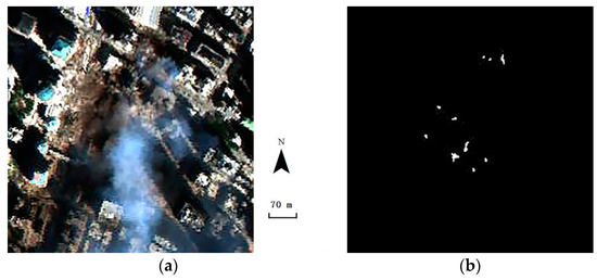
Figure 1. (a) AVIRIS image covering the World Trade Center (WTC) in New York City; (b) ground-truth map indicating spatial locations of hot spot fires, available from the United States Geological Survey.

3.1.2. SpecTIR Data

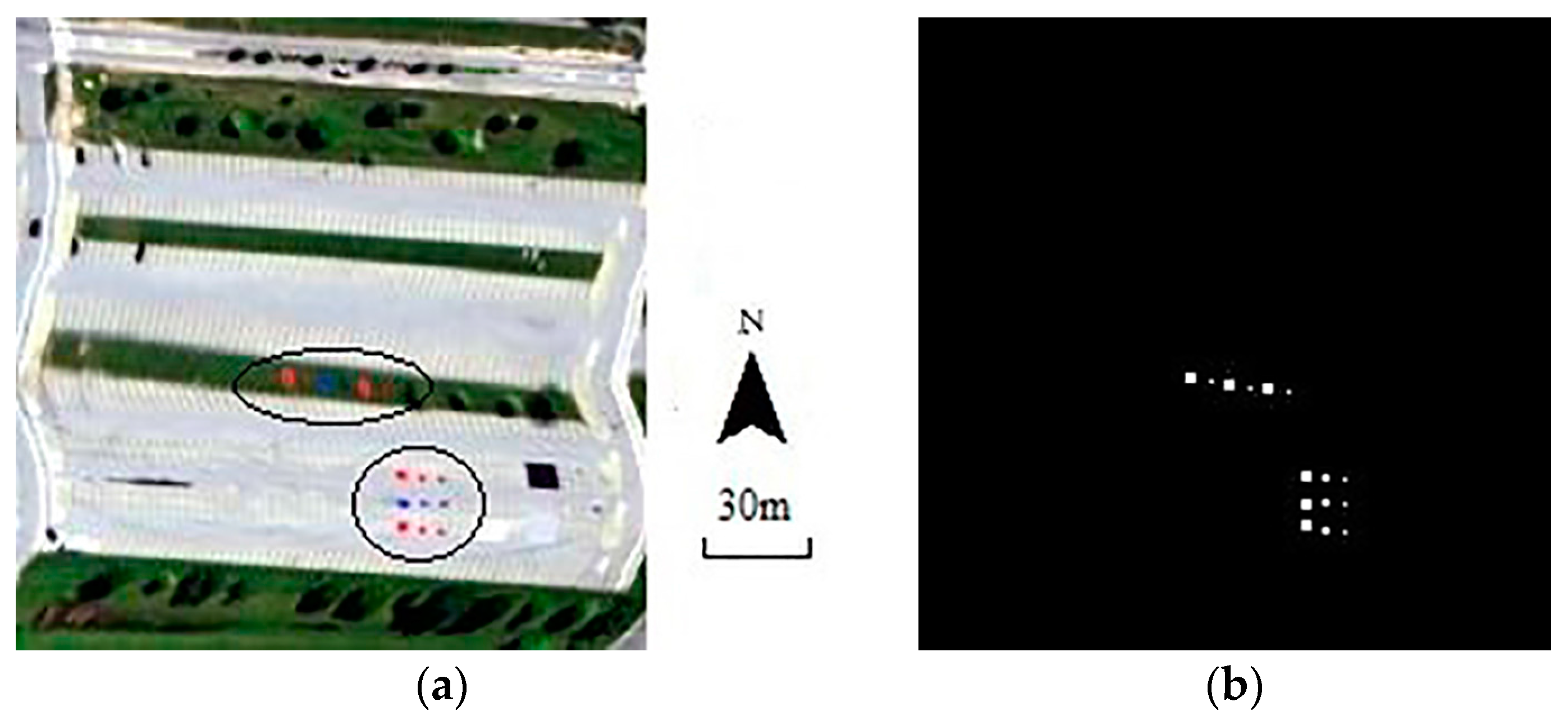
The second data set was collected in the SpecTIR Hyperspectral Airborne Rochester Experiment (SHARE) [13]. The data set was collected on 29 July 2010 by the ProSpecTIR-VS2 sensor containing 360 bands from 390–2450 nm with a 5 nm spectral resolution. The ground resolution is approximately 1 m. In the image, road and vegetation are the main backgrounds, and red and blue fabrics (sized 9, 4 and 0.25 m² respectively) were placed purposely as anomalies. We selected an area of 180 × 180 pixels that contains these anomalies, as displayed in Figure 2a, for the experiment. Figure 2b displays the ground-truth location of the anomalies in the experiment.

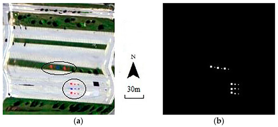
Figure 2. (a) The SpecTIR hyperspectral image. The anomalies were highlighted by black ellipses; (b) Ground-truth information of the anomalies.

3.2. Analyses of the ROC and the AUC

This section reports a comparison of the experimental results, created using the different detectors with two hyperspectral image scenes. Since the size of the anomalies in these two real images is usually more than one pixel, the local methods in the experiments were implemented using a dual window approach [14] to better estimate the background information. In our experiments, the inner and outer window sizes for the dual windows were set to 5 × 5 and 15 × 15 pixels, respectively, as they could lead to the best detection results for the data sets.

3.2.1. WTC

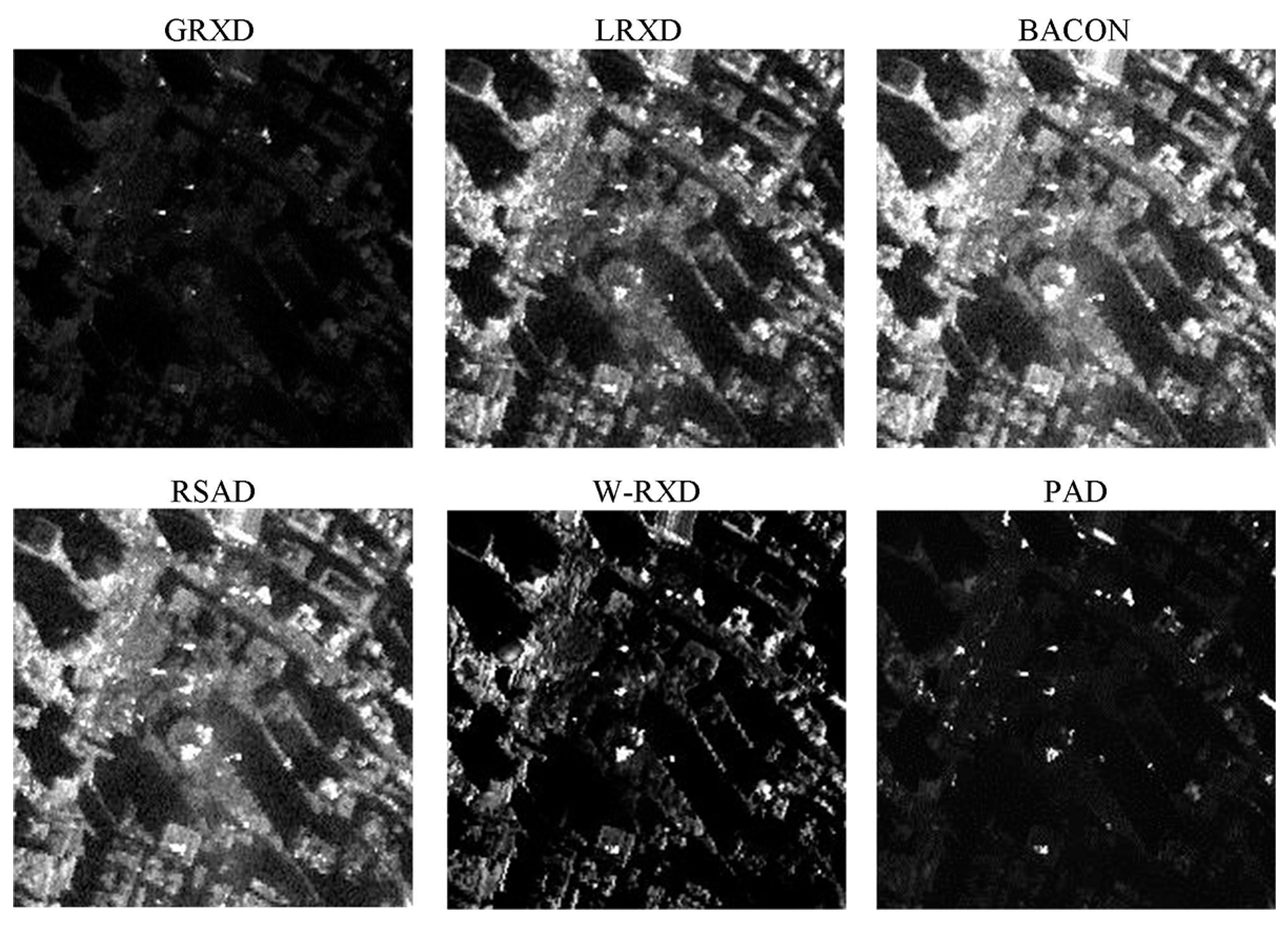
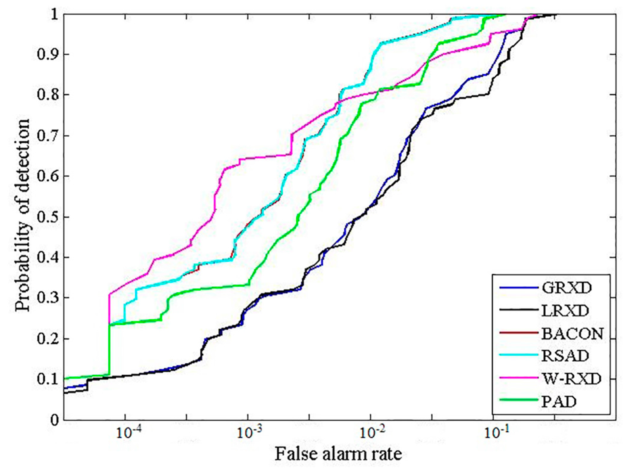
This study implemented the GRXD, LRXD, BACON, RSAD, W-RXD, and PAD and compared their results. There were at least two criteria that were used to evaluate the performances of the detection algorithms: receiver operating characteristic (ROC) curves [15] and the area under the ROC curves (AUC) [16]. The x-axis of the ROC is the false alarm rate (FAR), and the y-axis of ROC represents the probability of detection. Thus, it establishes a correspondence between the detection probability and the FAR. The upper and left curves indicate better detection performances. The grayscale images created using these detectors are shown in Figure 3. The statistic and stretching information for the six grayscale images is summarized in Table 1. We could identify some fire spots by their high brightness value. The ROCs of the discussed methods are presented in Figure 4, and their corresponding AUCs are shown in Table 2. From Table 2, the BACON and the RSAD shared the highest AUC value among all of the algorithms. However, the BACON took the longest time (97.03 s) among the six detectors, and the RSAD took some time, too (49.55 s). The main reason for this is that both the BACON and the RSAD are iterative algorithms, with great capabilities to purify the background albeit consuming much computation time. According to the AUC values and time consumption, the GRXD was better than the LRXD. The PAD outperformed the W-RXD with a larger AUC value, but the processing time was longer (20.91 s). The PAD and the W-RXD possess advantages when an image is large, as they keep the best balance on time consumption and detection performance among these detectors.

Figure 3. Detection results created by different algorithms with the WTC data.

Table 1. The statistic and stretching information of the six grayscale images for the WTC data set.

Algorithms	Min	Max	Mean	Stdev	Stretch From	Stretch To
GRXD	69.08	1.27 × 104	224.00	211.44	69.08	1.27 × 104
LRXD	68.33	466.45	216.60	203.95	68.33	466.45
BACON	8.45	622.36	15.12	9.87	8.45	22.90
RSAD	8.45	615.55	15.11	9.79	8.45	22.74
W-RXD	0.48	3.56 × 109	2.39 × 106	3.36 × 107	0.49	1.40 × 107
PAD	−258.32	2.39 × 105	136.17	2337.61	−258.32	3497.13

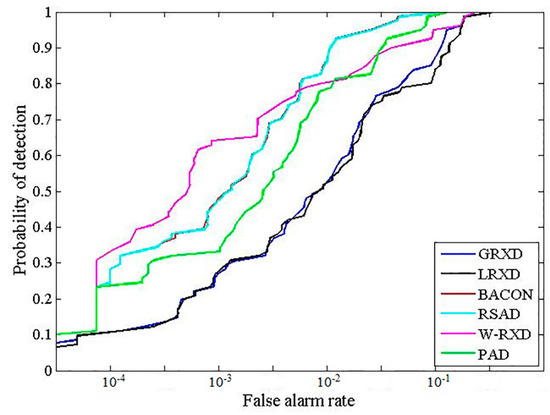
Figure 4. ROC curves corresponding to the detection results presented in Figure 3.

Table 2. AUCs and processing times (s) produced by the different detectors for the WTC data. See also Figure 3 and Figure 4.

Algorithms	AUC	Time (s)	Algorithms	AUC	Time (s)
GRXD	0.9689	9.11	LRXD	0.9642	36.10
BACON	0.9947	97.03	RSAD	0.9946	49.55
W-RXD	0.9837	14.10	PAD	0.9886	20.91

3.2.2. SpecTIR Data

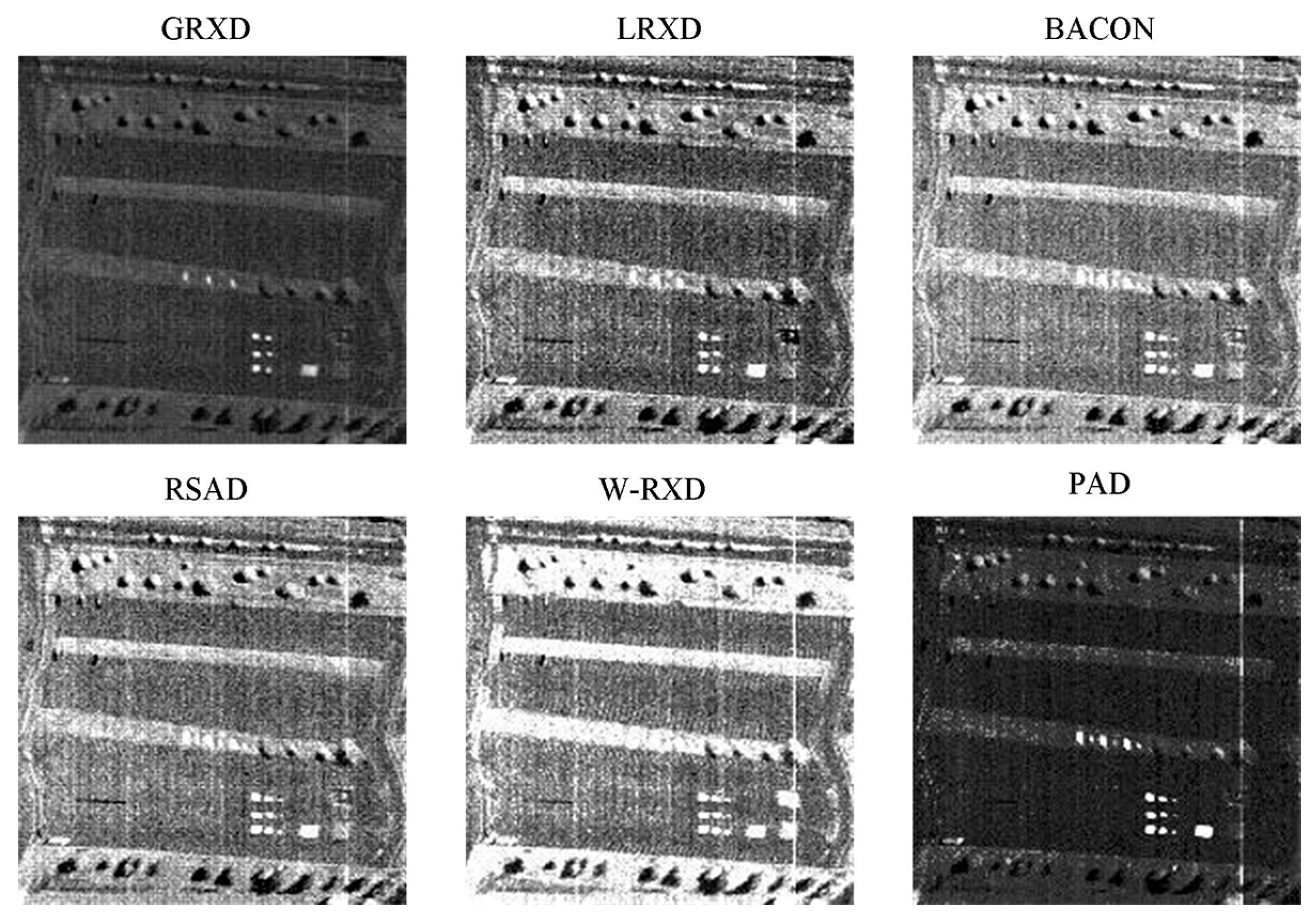
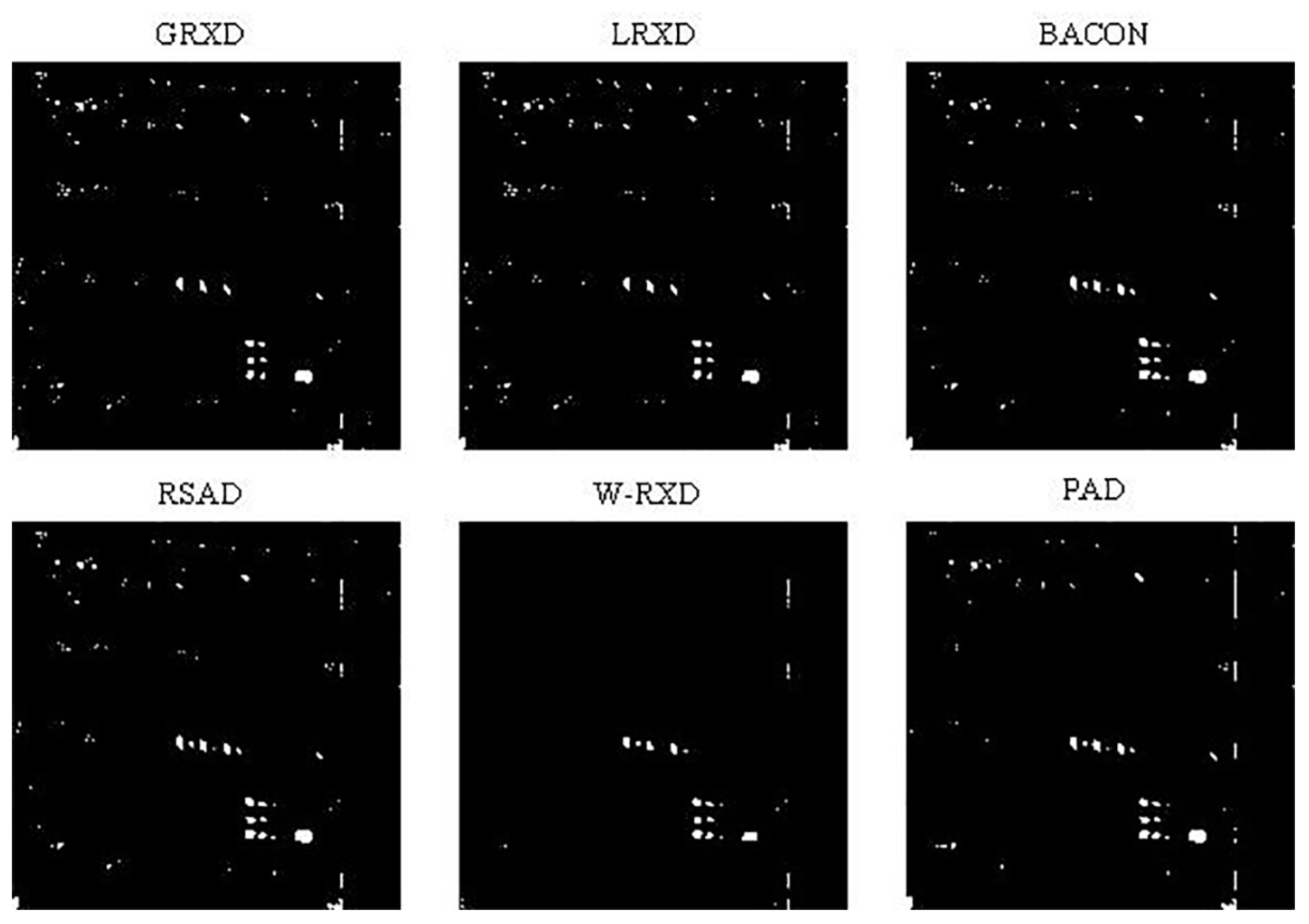
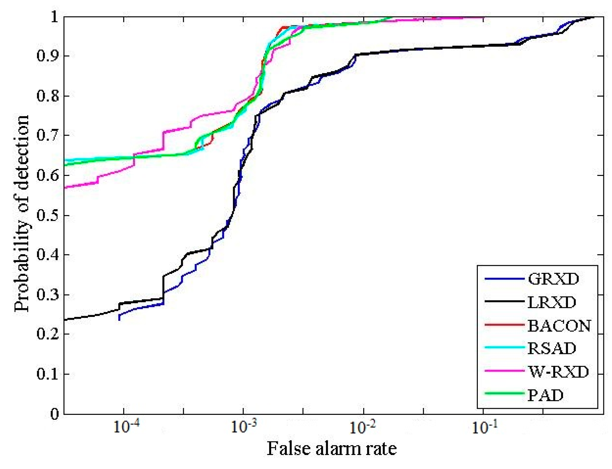
The detection results obtained from the SpecTIR image are presented in Figure 5. The binary images obtained after thresholding the detection results are shown in Figure 6. The statistic and stretching information for the six grayscale images is summarized in Table 3. From the binary images, it is noticeable that the BACON, RSAD, W-RXD, and PAD were able to detect a larger number of very small anomalies than the RXD and the LRXD. More specifically, the BACON, RSAD, W-RXD, and PAD were able to detect five sub-pixel panels (0.25 m²) out of six, while the GRXD and LRXD could not detect any of them. The ROC curves for the SpecTIR data are shown in Figure 7. Table 4 lists the AUC and the processing time of the six algorithms. The computational complexity of all six detectors is $O(N\cdot K^2)$, where N is the number of pixels, and K is the number of bands. Based on Figure 7 and Table 4, the performances of the BACON, RSAD, W-RXD, and PAD were almost the same for this data set. The four algorithms were better than the GRXD and the LRXD, which was indicated by the ROC curves and the AUC values. The BACON, RSAD, W-RXD, and PAD outperformed the GRXD and the LRXD in detecting sub-pixel anomalies. The AUC of GRXD was slightly larger than the AUC of the LRXD, and the GRXD also cost less time than the local algorithm. The BACON and the RSAD took more time than the W-RXD and the PAD because the BACON and the RSAD are iterative algorithms and conduct the detection process several times before termination. The PAD and W-RXD only perform the detection process twice as the first detection process aims to classify anomalies from the image (the PAD) or obtain weights for the pixels (the W-RXD). Thus, the PAD and the W-RXD can detect most of the anomalies and maintain the time-efficiency for the SpecTIR data.

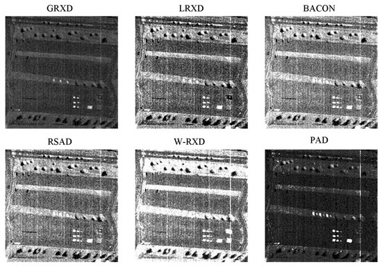
Figure 5. Detection results produced by different algorithms with the SpecTIR data.

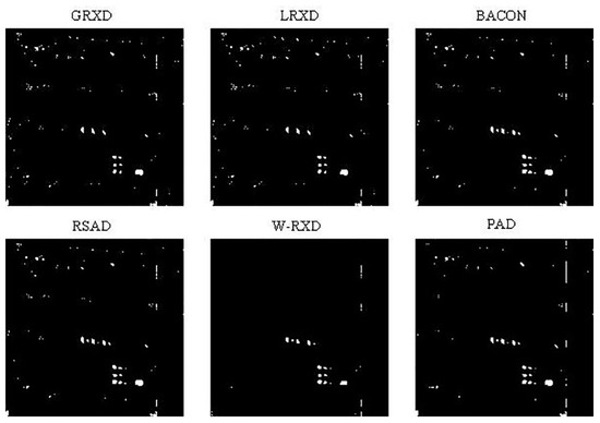
Figure 6. Binary images created after thresholding the results in Figure 5 using empirically selected thresholds. The ratio of anomaly was set to 1%.

Table 3. The statistic and stretching information of the six grayscale images for the SpecTIR data set.

Algorithms	Min	Max	Mean	Stdev	Stretch From	Stretch To
GRXD	125.37	3.30 × 103	360.92	117.62	125.38	3.30 × 103
LRXD	114.36	3.23 × 103	353.44	112.89	187.61	566.06
BACON	11.11	213.55	19.05	4.95	12.69	23.81
RSAD	11.11	194.33	19.03	4.62	13.26	24.04
W-RXD	13.85	1.19 × 106	3.89 × 103	1.75 × 104	13.85	4.67 × 103
PAD	−1.08×103	4.30 × 104	−3.04	618.28	−219.57	818.33

Figure 7. ROC curves corresponding to the detection results from the SpecTIR data presented in Figure 5 and Figure 6.

Table 4. AUCs and processing times (s) produced by the different detectors for the SpecTIR data.

Algorithms	AUC	Time (s)	Algorithms	AUC	Time (s)
GRXD	0.9683	12.28	LRXD	0.9651	67.80
BACON	0.9988	77.98	RSAD	0.9987	54.58
W-RXD	0.9986	30.28	PAD	0.9993	31.51

4. Discussion and Conclusions

This study applied anomaly detection algorithms with a hyperspectral image to detect fire spots and monitor the hazard using the WTC data. In fact, anomaly detection is a very important topic of research in hyperspectral image processing. Usually, it is performed under conditions without any prior background or target information. Currently existing algorithms (e.g., BACON, RSAD, and W-RXD) try to prevent contamination from anomalous signatures when estimating background information. The PAD estimates the information of both the background and the anomalies to eliminate the FAR. In this study, we used ROC, AUC, and consuming time as three criteria by which the performances of six detectors are evaluated. Two real hyperspectral data sets, the WTC data and the SpecTIR data, were processed by the detectors. The results of the two experiments showed that the BACON, RSAD, W-RXD, and PAD had better detecting capabilities than GRXD and LRXD. The performances of BACON, RSAD, W-RXD, and PAD were the same for the two data sets. However, since BACON and RSAD are iterative algorithms, and W-RXD and PAD are not, BACON and RSAD require more processing time than W-RXD and PAD do.

References

- Stein, D.W.J.; Beaven, S.G.; Hoff, L.E.; Winter, E.M.; Schaum, A.P.; Stocker, A.D. Anomaly detection from hyperspectral imagery. IEEE Signal Process. Mag. 2002, 19, 58–69. [Google Scholar] [CrossRef]
- Banerjee, A.; Burlina, P.; Diehl, C. A support vector method for anomaly detection in hyperspectral imagery. IEEE Trans. Geosci. Remote Sens. 2006, 44, 2282–2291. [Google Scholar] [CrossRef]
- Kwon, H.; Nasrabadi, N.M. Kernel RX-algorithm: A nonlinear anomaly detector for hyperspectral imagery. IEEE Trans. Geosci. Remote Sens. 2005, 43, 388–397. [Google Scholar] [CrossRef]
- Reed, I.S.; Yu, X. Adaptive multiple-band CFAR detection of an optical pattern with unknown spectral distribution. IEEE Trans. Acoust. Speech Signal Process. 1990, 38, 1760–1770. [Google Scholar] [CrossRef]
- Huck, A.; Guillaume, M. Asymptotically CFAR-unsupervised target detection and discrimination in hyperspectral images with anomalous-component pursuit. IEEE Trans. Geosci. Remote Sens. 2010, 48, 3980–3991. [Google Scholar] [CrossRef]
- Billor, N.; Hadi, A.S.; Velleman, P.F. BACON: Blocked adaptive computationally efficient outlier nominators. Comput. Stat. Data Anal. 2000, 34, 279–298. [Google Scholar] [CrossRef]
- Du, B.; Zhang, L. Random-selection-based anomaly detector for hyperspectral imagery. IEEE Trans. Geosci. Remote Sens. 2011, 49, 1578–1589. [Google Scholar] [CrossRef]
- Guo, Q.; Zhang, B.; Ran, Q.; Gao, L.; Li, J.; Plaza, A. Weighted-RXD and Linear Filter-Based RXD: Improving Background Statistics Estimation for Anomaly Detection in Hyperspectral Imagery. IEEE J. Sel. Top. Appl. Earth Obs. Remote Sens. 2004, 7, 2351–2366. [Google Scholar] [CrossRef]
- Gao, L.; Guo, Q.; Plaza, A.; Li, J.; Zhang, B. Probabilistic anomaly detector for remotely sensed hyperspectral data. J. Appl. Remote Sens. 2014, 8, 083538. [Google Scholar] [CrossRef]
- Gorelnik, N.; Yehudai, H.; Rotman, S.R. Anomaly detection in non-stationary backgrounds. In Proceedings of the 2010 2nd Workshop on Hyperspectral Image and Signal Processing: Evolution in Remote Sensing, Reykjavìk, Iceland, 14–16 June 2010.
- Manolakis, D.; Lockwood, R.; Cooley, T.; Jacobson, J. Is there a best hyperspectral detection algorithm? Proc. SPIE 2009, 7334. [Google Scholar] [CrossRef]
- Molero, J.M.; Garzon, E.M.; Garcıa, I.; Plaza, A. Analysis and optimizations of global and local versions of the RX algorithm for anomaly detection in hyperspectral data. IEEE J. Sel. Top. Appl. Earth Obs. Remote Sens. 2013, 6, 801–814. [Google Scholar] [CrossRef]
- Herweg, J.A.; Kerekes, J.P.; Weatherbee, O.; Messinger, D.; van Aardt, J.; Ientilucci, E.; Ninkov, Z.; Faulring, J.; Raqueno, N.; Meola, J. SpecTIR hyperspectral airborne rochester experiment data collection campaign. Proc. SPIE 2012, 8390. [Google Scholar] [CrossRef]
- Kwon, H.; Der, S.Z.; Nasrabadi, N.M. Adaptive anomaly detection using subspace separation for hyperspectral imagery. Opt. Eng. 2003, 42, 3342–3351. [Google Scholar] [CrossRef]
- Molero, J.M.; Garzon, E.M.; Garcia, I.; Plaza, A. Anomaly detection based on a parallel kernel RX algorithm for multicore platforms. J. Appl. Remote Sens. 2012, 6. [Google Scholar] [CrossRef]
- Khazai, S.; Homayouni, S.; Safari, A.; Mojaradi, B. Anomaly detection in hyperspectral images based on an adaptive support vector method. IEEE Geosci. Remote Sens. Lett. 2011, 8, 646–650. [Google Scholar] [CrossRef]
© 2016 by the authors; licensee MDPI, Basel, Switzerland. This article is an open access article distributed under the terms and conditions of the Creative Commons Attribution (CC-BY) license (http://creativecommons.org/licenses/by/4.0/).