Evaluation of Groundwater Quality for Drinking and Irrigation Purposes Using Entropy-Weighted WQI, Pollution Index, and Multivariate Statistical Analysis in the Maze Zenti Catchment, Southern Ethiopia

Abstract

Population growth and agricultural expansion are threatening groundwater resources in the Maze Zenti catchment, Southern Ethiopia. This study evaluated groundwater suitability for drinking and irrigation by analyzing 30 samples using an integrated approach. This approach included GIS-based IDW interpolation, hydrochemical characterization, drinking water quality index, entropy weight, pollution index of groundwater, multivariate statistics, Piper, Gibbs, and Wilcox diagrams, ANOVA, and irrigation indices based on WHO standards. The correlation matrix revealed strong associations between Na⁺-TDS (r = 0.77) and Na⁺-Ca²⁺ (r = 0.68), indicating mineral dissolution, ion exchange, and agricultural inputs as key factors. Weak correlations were found for NO₃⁻ and F⁻, reflecting localized anthropogenic and geogenic influences. Component analysis identified four components explaining 78.2% (wet season) and 81.2% (dry season) of the variance, highlighting mineralization and anthropogenic inputs. Hydrochemical facies were mainly Ca-Mg-HCO₃ with some localized Na-HCO₃, suggesting that rock–water interactions are the primary source of geochemical control. Drinking water quality assessment showed that, during the wet season, 52.8% of the catchment had excellent water quality, 45.8% was good, and 1.4% was poor–very poor. In the dry season, 51.6% was excellent, 47.4% was good, 0.8% was poor, and 0.2% was very poor. The results of the entropy-weighted analysis indicated seasonal improvement, with excellent areas increasing from 13.1% to 31.4% and poor zones decreasing from 7.5% to 3.4%. Irrigation indices (Na%, PI, MAR, SAR) and Wilcox analysis (86.4% C2S1) suggested low sodicity and salinity hazards. This study provides the first integrated seasonal mapping of drinking and irrigation water quality, entropy-weighted water quality, and pollution index for the Maze Zenti catchment, establishing a hydrogeochemical baseline. Overall, groundwater in the area is generally suitable for drinking and irrigation. However, localized monitoring and sustainable land-use practices are recommended to mitigate contamination risks.

1. Introduction

Groundwater is a crucial natural resource, serving as a primary source of water for domestic, agricultural, and industrial uses worldwide [1,2,3]. In arid and semi-arid regions where surface water is scarce, groundwater often serves as the only reliable freshwater source [4]. However, groundwater quality varies significantly due to natural factors such as precipitation, aquifer properties, rock–water interactions, climate, and topography, as well as human activities [5,6,7,8]. Therefore, assessing groundwater suitability for drinking and irrigation is crucial, especially in areas prone to contamination. In many developing countries, including those in sub-Saharan Africa, groundwater quality assessment and management are inadequate [9,10,11]. Challenges include insufficient monitoring, poor identification of contamination sources, limited vulnerability assessments, and weak infrastructure oversight. Because of this, contamination from both natural and man-made sources continues, endangering both agricultural output and public health [12,13,14,15,16,17].

Various methods exist to evaluate groundwater quality, each with advantages and limitations. The Water Quality Index (WQI) condenses complex water quality data into a single metric, providing an accessible measure of drinking water suitability [18,19]. Remote sensing (RS) and Geographic information Systems (GIS) facilitate spatial analysis and visualization of hydrochemical data, aiding in the identification of contamination patterns over large areas [19,20,21,22]. Recent advances include machine learning models such as Random Forest and Support Vector Machines, which enhance predictive accuracy and source identification [23]. Integrated approaches combining entropy-based weighting, multi-criteria decision analysis (MCDA), and hydrochemical data have proven especially useful in data-limited regions, offering clear, cost-effective, and decision-friendly visualizations of groundwater quality [24,25,26]. While advanced models provide predictive power, traditional WQI remains highly practical for baseline groundwater assessment and management planning. The present study newly integrates GIS-based spatial interpolation, hydrochemical characterization, WQI, entropy weighting, pollution indices, and multivariate statistical analysis, allowing a comprehensive evaluation of both drinking and irrigation water quality in the Maze Zenti catchment.

Although groundwater plays a vital role in the Maze- Zenti region of the Omo River Basin in Southern Ethiopia, its hydrogeochemistry, geographical distribution, and suitability for irrigation and drinking have not been thoroughly studied [27,28,29,30]. Concerns regarding groundwater sustainability are raised by the region’s increasing water consumption as a result of population growth and agricultural expansion. Local aquifers, including shallow unconfined wells, springs, and deeper semi-confined and confined systems, are influenced by complex lithology, including volcanic rocks (basalt, ignimbrite, and rhyolite), granite, and weathered gneiss. Available data on seasonal variations, geochemical controls, and contamination sources are limited, preventing effective water resource management. Using indices such as Permeability Index (PI), Sodium Adsorption Ratio (SAR), Sodium Percentage (Na%), Kelly Ratio (KR), Magnesium Adsorption Ratio (MAR), and Residual Sodium Carbonate (RSC), which offer insights into soil–water interactions and possible agricultural impacts, it is also essential to evaluate irrigation suitability.

This study aims to fill these knowledge gaps by conducting the first comprehensive hydrogeochemical assessment of groundwater in the Maze Zenti catchment. Specifically, the study objectives are to (i) evaluate physicochemical water quality using entropy-weighted WQI and pollution indices, (ii) identify the major geochemical processes influencing groundwater composition through statistical and hydrochemical analyses, and (iii) examine spatial patterns and potential contamination sources using multivariate statistical techniques and GIS-based interpolation. The integrated approach provides a robust understanding of groundwater suitability for drinking and irrigation, informs sustainable water management practices, and offers baseline data to support monitoring, planning, and policy development in the region.

2. Martials and Methods

2.1. Description of the Study Area

The Maze Zenti watershed is located in the Southern Ethiopia regional state’s Omo River Basin (Figure 1). Geographically, the study area extends from 6°00′00″ to 6°40′00″ N latitude and from 36°50′00″ to 37°30′00″ E longitude. The 2340 square kilometers compose the whole surface area. Asphalt roads that connect Arba Minch to Kamba and Sawula enable easy field research access to the Maze Zenti Catchment (Figure 1). Agriculture and domestic use are the largest water consumers in the Maze Zenti catchment. Groundwater supports small-scale irrigation along the Maze and Zenti rivers, enabling the cultivation of maize, wheat, nuts, and vegetables, which are vital for rural livelihoods. With a total population of 756,889 and a population density of 324 people per km² (Gamo and Gofa Zones Agricultural Office), springs and groundwater serve as the primary sources for drinking water, highlighting the importance of assessing aquifer water quality for both human use and agriculture activities.

The Maze Zenti Catchment has a bimodal rainfall pattern and receives a mean of 950 mm of precipitation annually. The wet season (June–September) records a mean rainfall of 216.8 mm and an average temperature of 20.2 °C, whereas the dry season (October–May) receives about 169.8 mm of rainfall with a mean temperature of 24.1 °C. The Maze and Zenti Rivers form a intricate drainage network that ultimately drains into the Omo River.

2.2. Geology and Hydrogeology Setting of Study Area

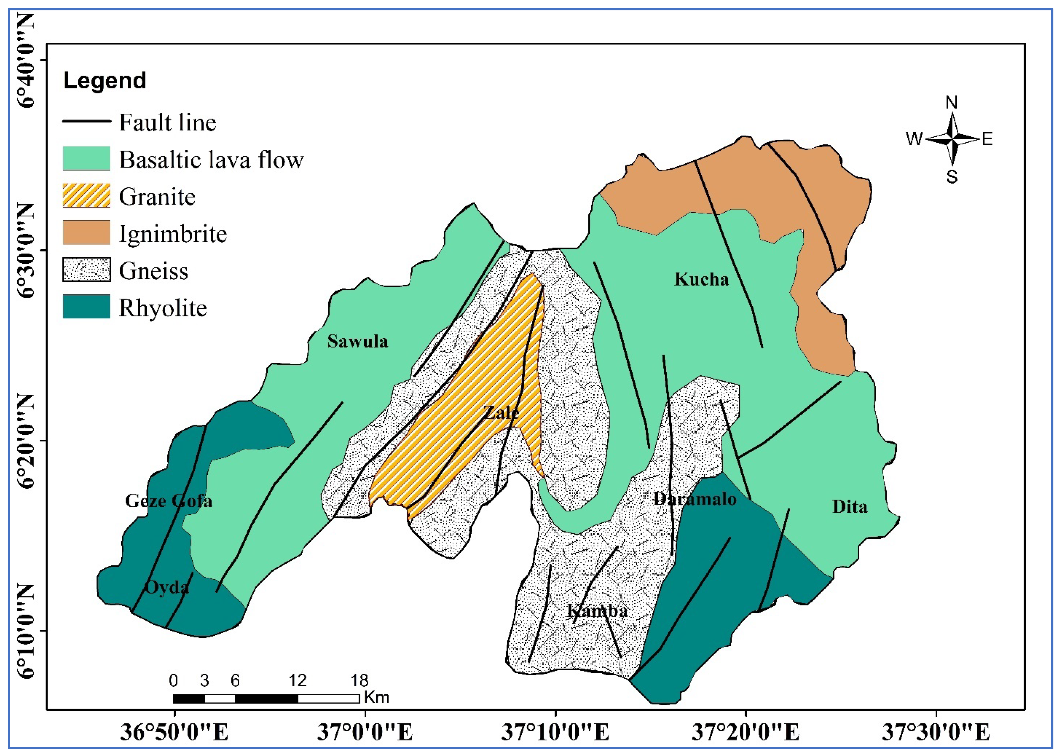
The Maze Zenti catchment exhibits a complex geological framework characterized by volcanic, metamorphic, and intrusive rocks ranging from the Precambrian to the Quaternary period [31,32]. The primary lithological units include Precambrian gneiss, granite, Tertiary ignimbrites, rhyolite, basaltic lava flows, and unconsolidated Quaternary alluvial deposits (Figure 2). The Precambrian gneisses form the oldest basement, overlain by granitic intrusions and Tertiary volcanic sequences. Quaternary alluvial deposits occupy the low-lying river valleys and form thick accumulations along riverbanks, mountain foot slopes, and gully mouths. These unconsolidated sediments, consisting of sand, silt, clay, gravel, and boulders, play a crucial role in local groundwater recharge, particularly in fine-grained layers.

The catchment is influenced by multiple faults, joints, and fractures associated with tectonic activity in the western escarpment of the Ethiopian Rift within the Omo River Basin. Major northeast-southwest trending fault systems dominate the geological framework and significantly control both surface morphology and subsurface hydrology. Notably, the Jima Volcano represents a key geological feature, comprising interbedded rhyolitic and basaltic flows with Miocene-Pliocene ignimbrites, reflecting the region’s younger volcanic phase [31,32]. Tectonic pressures enhance secondary porosity along joints and fault zones in the extensively worn and fractured volcanic formations, especially in the catchment’s northwest and eastern areas.

The metamorphic basement, which includes the Alghe Group’s biotite and hornblende gneiss, is primarily visible in the catchment’s central and southern regions due to pre-tectonic granite intrusions. These rocks exhibit deep weathering, quartz–calcite veining, and localized deformation structures. Contacts between volcanic and metamorphic units often serve as preferential zones for groundwater discharge, with numerous springs emerging along fractures and fault planes. Overall, the interplay between lithology, tectonic structures, and weathering processes establishes the geological foundation for the catchment’s hydrogeological behavior.

The hydrogeology of the Maze Zenti catchment is largely governed by the lithological and structural characteristics of its subsurface formations. The Precambrian gneiss and granite constitute the basement complex and generally act as low-permeability aquicludes, restricting groundwater movement except where secondary porosity is enhanced by faulting and fracturing. Overlying Tertiary volcanic rocks sequences including ignimbrites, rhyolites, and basaltic lava flows exhibit vesicular and fractured textures that provide substantial secondary permeability, making them significant groundwater storage. Quaternary alluvial sediments composed of sand, silt, and gravel form highly permeable zones, hosting shallow unconfined aquifers that receive recharge from rainfall and river infiltration, supporting year-round water availability.

Field observations and previous drilling indicate that fractured basalt formations and alluvial sediments of sand and gravel constitute the principal aquifers in the Maze Zenti catchment (Figure 2). Open fractures, joints, and weathered zones in basalt enhance groundwater storage and circulation, while ignimbrite and rhyolitic units locally store water within fractured or weathered sections. Borehole records show weathered and fractured basaltic zones range from 12 to 50 m thick, with wells yielding up to 8.5 L/s, and nearby springs discharging 1.4–5.6 L/s. Alluvial deposits along the Maze and Zenti Rivers form productive shallow aquifers recharged by rainfall and river infiltration. In contrast, gneiss and granite act mainly as aquitards, limiting groundwater flow except where faults and fractures provide secondary pathways. Overall, secondary porosity in volcanic and alluvial units represents the most promising groundwater source in the catchment. The area is characterized by two main aquifer systems: shallow unconfined aquifers occurring in weathered and fractured basalt and ignimbrite, and deeper semi-confined aquifers in gneiss and granite formations. Shallow aquifers are more vulnerable to contamination from the land surface, whereas deeper aquifers are less susceptible. This study provides new baseline information on groundwater quality in the area.

Groundwater recharge in the Maze Zenti catchment primarily occurs through direct infiltration of rainfall and percolation through permeable volcanic and alluvial formations. Elevated recharge zones are concentrated in highland areas underlain by fractured basaltic and ignimbrite rocks, where jointing, faulting, and weathered zones enhance water infiltration. Faults and fractures act as preferential pathways, facilitating the downward movement of water into deeper aquifer systems. From the highlands of Dita, Daramalo, Zala, and Kucha toward the Maze River, and from Oyda and Geze Gofa Zala toward the Zenti River, regional groundwater flow often adheres to the topographic gradient. Discharge areas are mainly found along river valleys and in low-lying alluvial plains, where surface water is maintained during the dry season through springs and river base flow.

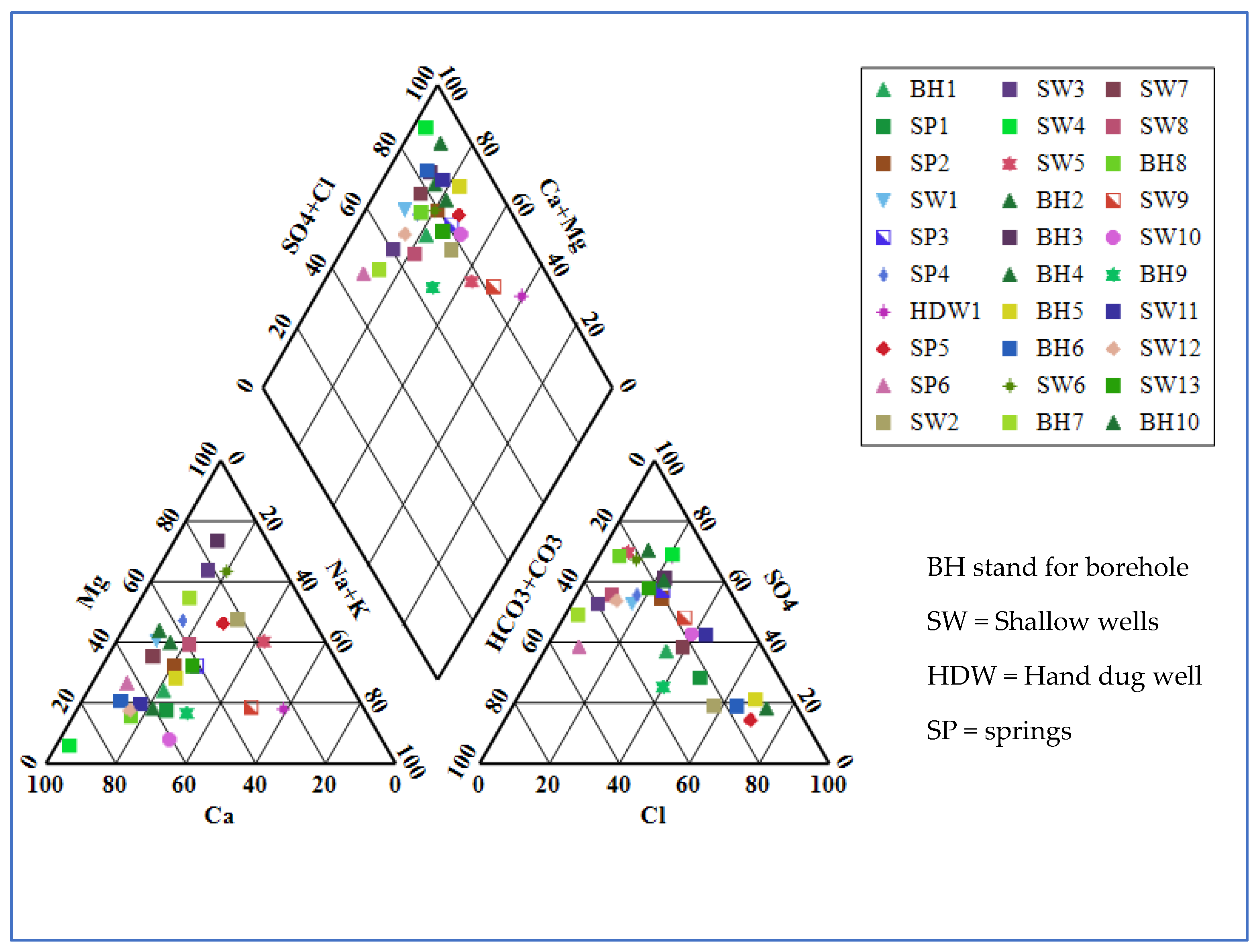
An essential part of the hydrogeological system of the catchment is the connection between the surface water and subsurface water. In upstream volcanic terrains, rivers often lose water to fractured aquifers during periods of high recharge, while in downstream alluvial plains, groundwater discharges into rivers and springs, maintaining continuous base-flow. These flow dynamics directly influence hydrochemical processes, including silicate weathering in basaltic and rhyolitic rocks, ion exchange in fractured ignimbrites, and carbonate dissolution in alluvial deposits. Fault and fracture-controlled flow enhance mineral dissolution and mix between shallow and deep aquifers, generating spatial variations in water chemistry. The cumulative effects of lithological heterogeneity, aquifer characteristics, recharge–discharge dynamics, and structural controls within the research area are thus reflected in the observed hydrochemical facies and geochemical history.

2.3. Data Collection and Analysis

The study began with the collection of secondary data and compilation of hydrogeological and geological information from previous water supply studies. Springs and wells were mapped to assist in identifying locations for groundwater sample collection. The study area was divided into zones based on hydrogeological and geological factors. The sample points were chosen based on physiographic area (highlands, escarpment, and lowlands), lithology, population density, and land use. Groundwater samples were collected from various aquifers, including shallow wells and hand-dug wells representing unconfined shallow aquifers, boreholes representing semi-confined–confined aquifers, and springs representing recharge areas. The study included a variety of aquifers to ensure a range of water compositions, both natural and human-induced, were analyzed. More sample points were allocated to areas with higher levels of groundwater components.

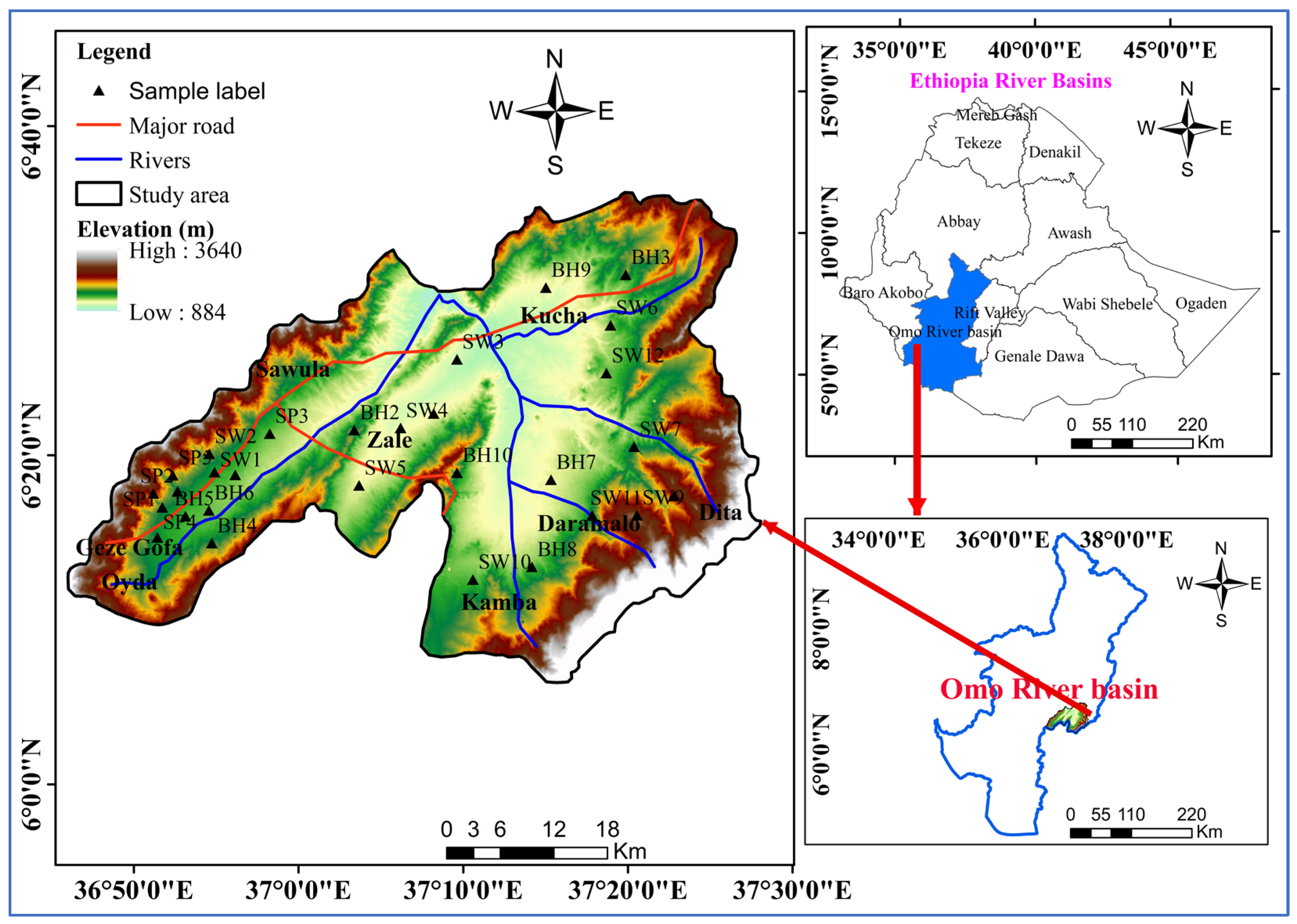
A total of 30 water locations in the Maze Zenti watershed were used for collecting samples of groundwater during the wet (October 2024) and dry (February 2025) seasons. These included six springs that emerged from fractured basalt along fault zones and twenty-four shallow, hand-dug, and deep wells (Figure 1). Sampling sites were selected based on hydrogeological significance, accessibility, and operational status, although limited infrastructure and non-functioning sources restricted sampling of the southern and eastern portion of the area. These water sources are vital for local communities, providing drinking water and meeting daily household needs, with springs and groundwater-fed rivers flowing continuously throughout the year.

To account for aquifer variability, a water level meter was used to determine the depth to the water table at each sampling location, and the construction type and installation year were noted (Table 1). This study used purging approach in which more than three times the well volume was pumped from each borehole and shallow well in order to reduce the possible impact of accumulated water in the borehole during sampling. Sampling was conducted only after field parameters stabilized over three consecutive readings, with pH varying by no more than ±0.1 units, electrical conductivity (EC) within ±3%, and temperature within ±0.2 °C. Springs were sampled directly after discharge stabilized to capture fresh aquifer water. Geographic coordinates of all sites were recorded using a handheld GPS to support spatial analyses. These standardized procedures ensured that the samples collected accurately represented natural groundwater conditions across both inactive and active sources.

To avoid contamination, all samples were collected in 1 L polyethylene bottles that have been properly cleaned and rinsed three times with distilled water. The samples were then rapidly stored in portable refrigerators at 4 °C. After established procedures, the samples were transported to the laboratory of the Arba Minch Water Technology Institute (AWTI), Faculty of Water Supply and Environmental Engineering, for chemical analysis. A Hanna pH meter (Model HI99300, Hanna Instruments, Kallang Avenue, Singapore) with daily calibration was used to monitor physical parameters in situ, including pH, temperature, electrical conductivity, total dissolved solids (TDS), and total hardness.

The chemical composition of groundwater samples was analyzed following standard procedures. Sodium (Na⁺) and potassium (K⁺) concentrations were determined using atomic absorption spectrophotometry (PerkinElmer A Analyst 400, EPA 200.7, PerkinElmer, New York, NY, USA) and flame photometry (Sherwood 410, ISO 6384) with a detection limit of 0.01 mg/L. Calcium (Ca²⁺) and magnesium (Mg²⁺) were measured by EDTA titration (Standard Method 2340C) with a detection limit of 0.1 mg/L. Chloride (Cl⁻) was determined by titration with silver nitrate (SM 4500-Cl⁻ B, detection limit 0.1 mg/L), and bicarbonate (HCO₃⁻) and carbonate (CO₃²⁻) were determined by acid titration (SM 2320B, detection limit 1 mg/L). Nitrate (NO₃⁻), sulfate (SO₄²⁻), and iron (Fe²⁺) concentrations were measured using a UV-VIS spectrophotometer (Hach DR 6000, EPA 353.2, Hach, Loveland, CO, USA) with a detection limit of 0.01 mg/L, while fluoride (F⁻) was analyzed using the ion-selective electrode method (Orion 9609BN, SM 4500-F⁻ E, Thermo Fisher Scientific, Waltham, MA, USA) with a detection limit of 0.02 mg/L.

Total hardness and alkalinity were calculated and expressed as mg/L of CaCO₃ equivalent using standard conversion factors. To ensure analytical reliability, all instruments were calibrated prior to analysis, and blanks, duplicates, and standards were measured for quality control. Additionally, the ion balance error (IBE) was calculated, as shown in Equation (1), to verify charge neutrality between cations and anions [8,33,34]. Acceptable IBE values confirmed the accuracy and reproducibility of the chemical analyses, providing reliable data for subsequent hydrochemical interpretation.

$$\left(\mathrm{I}\mathrm{B}\mathrm{E}\right)={\displaystyle \frac{\sum \mathrm{C}\mathrm{a}\mathrm{t}\mathrm{i}\mathrm{o}\mathrm{n}-\sum \mathrm{a}\mathrm{n}\mathrm{i}\mathrm{o}\mathrm{n}\mathrm{s}}{\sum \mathrm{C}\mathrm{a}\mathrm{t}\mathrm{i}\mathrm{o}\mathrm{n}+\sum \mathrm{a}\mathrm{n}\mathrm{i}\mathrm{o}\mathrm{n}\mathrm{s}}}\times 100\%; \le \pm 5$$

(1)

where ∑Cations is the total concentration of cations (Na⁺, K⁺, Ca²⁺, Mg²⁺ in meq/L) and ∑Anions represents the total concentration of anions (${\mathrm{C}\mathrm{l}}^{-}$, ${\mathrm{H}\mathrm{C}\mathrm{O}}_3^{-}$, and ${\mathrm{S}\mathrm{O}}_4^{2-}$ liter meq/L).

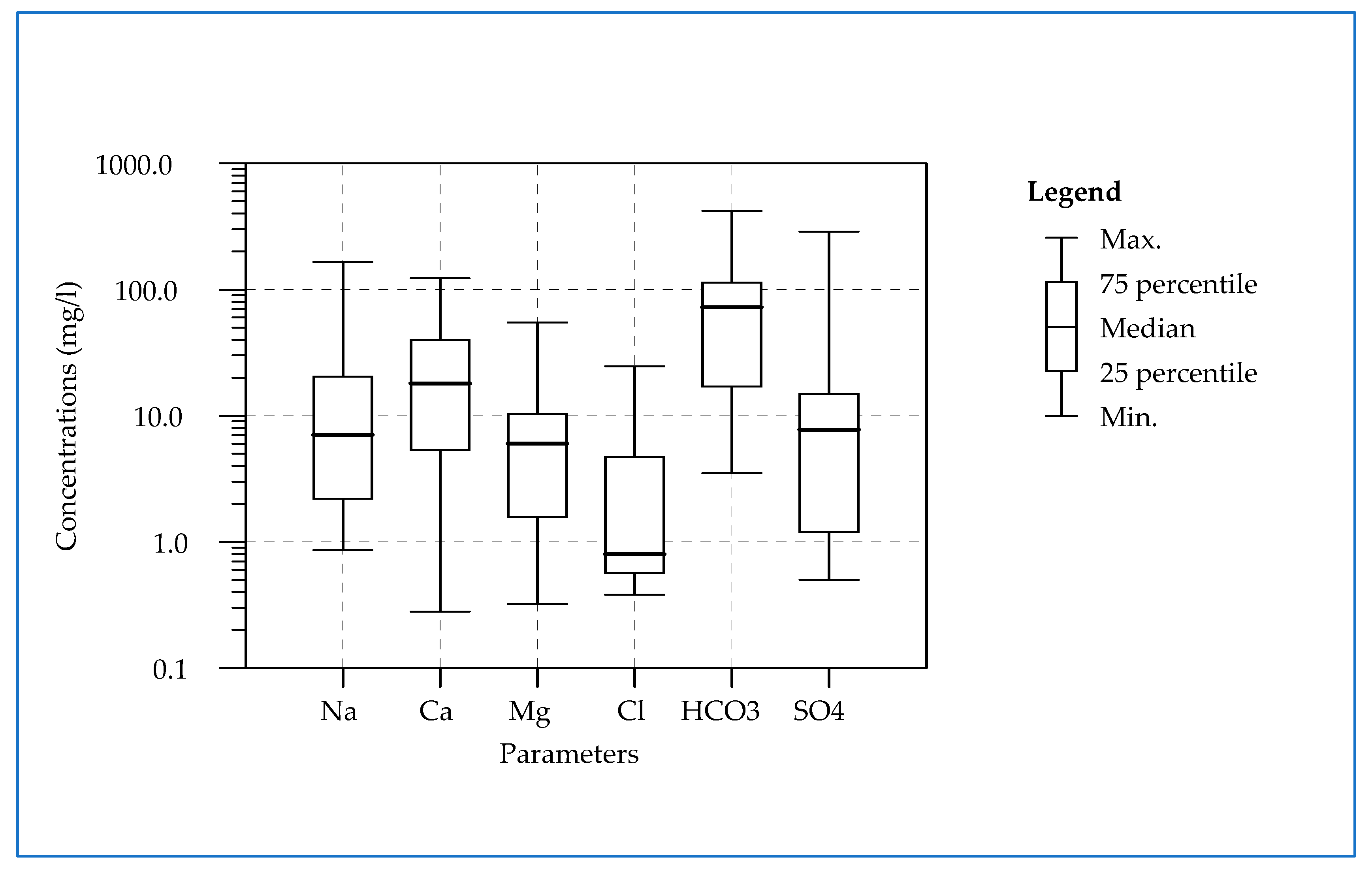
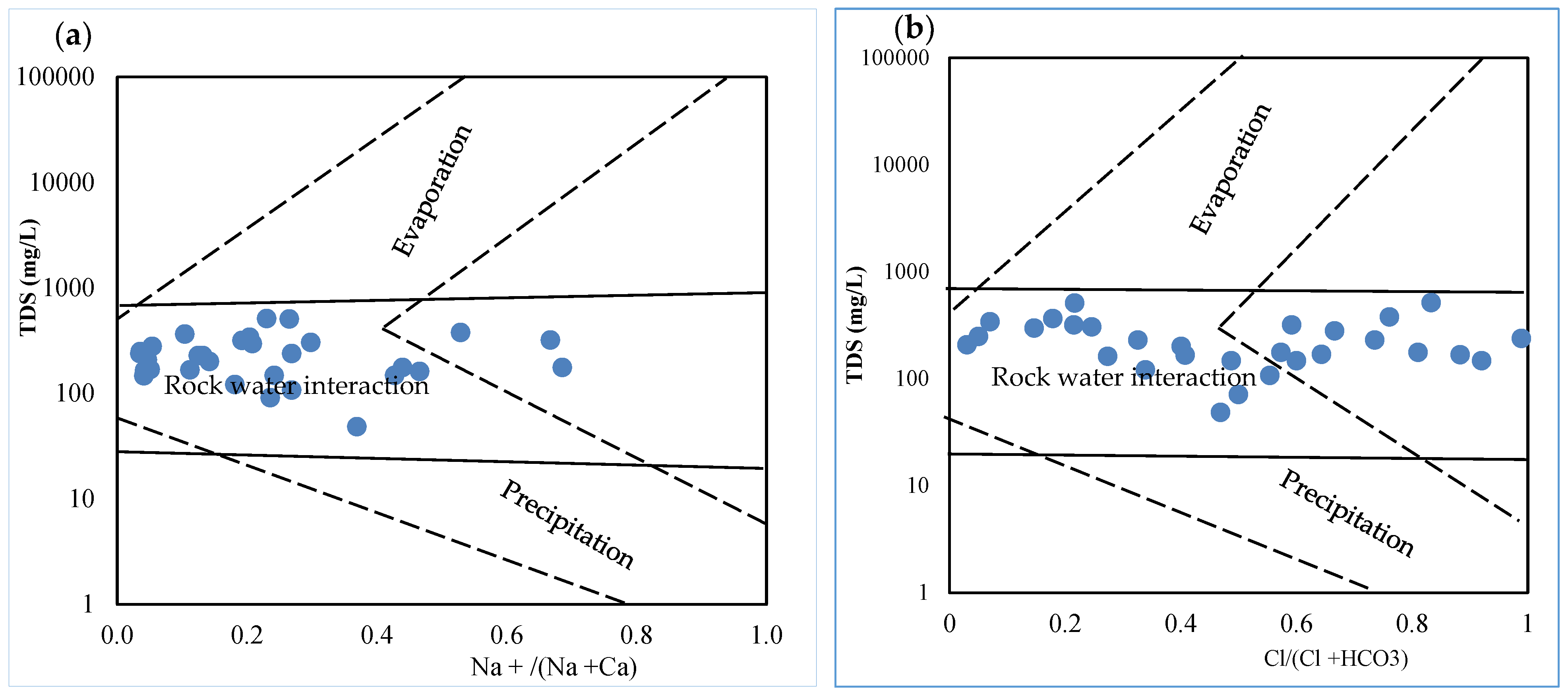
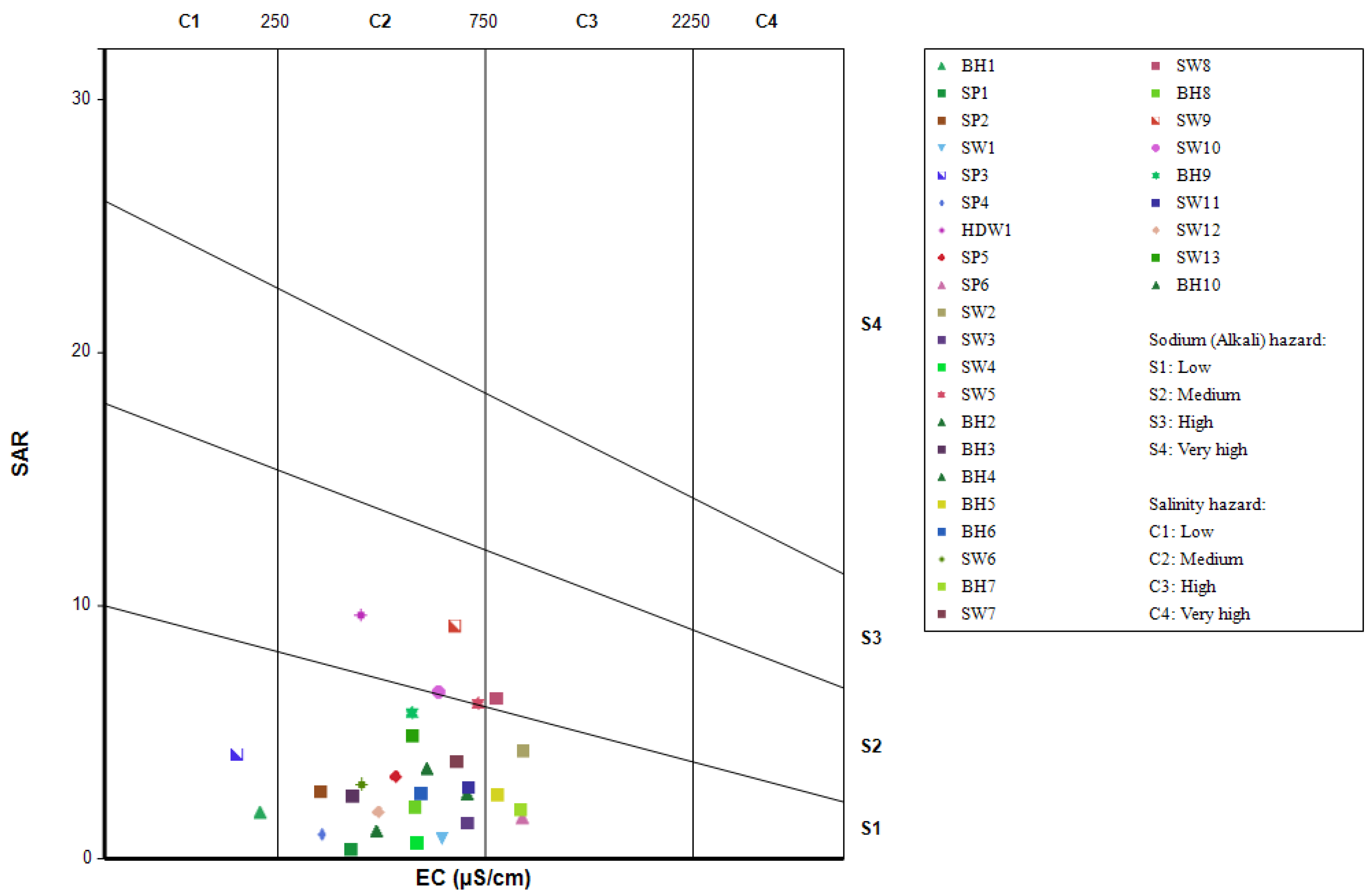
Descriptive statistical analyses were employed to examine the variability and relationships among groundwater quality parameters, while hydrochemical diagrams such as Piper, Wilcox, and Wishek plots were generated using AquaChem 4.0, and Gibbs scatter plots were prepared using Microsoft Excel to classify groundwater facies and interpret geochemical processes. Collectively, these tools facilitated the identification of salinity sources, cation exchange mechanisms, and anthropogenic influences on groundwater chemistry [35,36,37]. Before performing the one-way ANOVA to assess seasonal variations, the normality of each water quality parameter was evaluated using the Shapiro–Wilk test in Excel with the Real Statistics Resource Pack (https://real-statistics.com/free-download/real-statistics-resource-pack) (accessed on 6 January 2026). The add-in was installed by Excel’s Add-ins tool, and descriptive analysis was applied to conduct the Shapiro–Wilk test for all samples. The results yielded p-values above 0.05 for all parameters, confirming that the data were approximately normally distributed and met the assumptions required for parametric analyses such as ANOVA and PCA, thereby ensuring the validity and reliability of the statistical results. Subsequently, a one-way ANOVA was applied to compare groundwater quality between wet and dry seasons and among different sampling sites at a 95% confidence level (p < 0.05), providing a statistically robust evaluation of spatial and seasonal variations in groundwater characteristics [38,39].

Table 1. Location, elevation, depth, construction type, and year of installation of groundwater sampling points in the Maze Zenti catchment.

SN	Latitude (°N)	Longitude (°E)	Elevation (m)	Depth (m)	Construction Type	Year of Installation
1	6.3	36.9	2382	150	Borehole	2014
2	6.3	36.9	2251	Surface	Spring	Unknown
3	6.3	36.9	1847	Surface	Spring	Unknown
4	6.3	36.9	1918	60	Shallow well	2019
5	6.4	37.1	2064	Surface	Spring	Unknown
6	6.3	36.9	2147	Surface	Spring	Unknown
7	6.3	36.9	2361	3	Hand dug well	2022
8	6.3	36.9	2358	Surface	Spring	Unknown
9	6.4	37.1	1361	Surface	Spring	Unknown
10	6.3	36.9	2468	70	Shallow well	2018
11	6.4	37.2	1210	62	Shallow well	2021
12	6.4	37.1	1229	60	Shallow well	2017
13	6.3	37.1	1278	65	Shallow well	2023
14	6.4	37.1	1235	120	Borehole	2017
15	6.5	37.3	1385	150	Borehole	2018
16	6.2	36.9	1044	280	Borehole	2020
17	6.3	36.9	1245	180	Borehole	2016
18	6.3	36.9	1237	150	Borehole	2017
19	6.5	37.3	1426	50	Shallow well	2019
20	6.3	37.3	1189	150	Borehole	2015
21	6.3	37.3	1623	63	Shallow well	2019
22	6.6	37.4	983	65	Shallow well	2018
23	6.2	37.2	1540	138	Borehole	2020
24	6.3	37.3	1820	75	Shallow wells	2019
25	6.2	37.2	1390	60	Shallow wells	2021
26	6.5	37.2	1516	150	Borehole	2023
27	6.3	37.3	1470	55	Shallow wells	2021
28	6.4	37.3	1720	50	Shallow wells	2020
29	6.3	37.4	1382	60	Shallow wells	2014
30	6.3	37.2	1412	180	Borehole	2015

Table 1. Location, elevation, depth, construction type, and year of installation of groundwater sampling points in the Maze Zenti catchment.

SN	Latitude (°N)	Longitude (°E)	Elevation (m)	Depth (m)	Construction Type	Year of Installation
1	6.3	36.9	2382	150	Borehole	2014
2	6.3	36.9	2251	Surface	Spring	Unknown
3	6.3	36.9	1847	Surface	Spring	Unknown
4	6.3	36.9	1918	60	Shallow well	2019
5	6.4	37.1	2064	Surface	Spring	Unknown
6	6.3	36.9	2147	Surface	Spring	Unknown
7	6.3	36.9	2361	3	Hand dug well	2022
8	6.3	36.9	2358	Surface	Spring	Unknown
9	6.4	37.1	1361	Surface	Spring	Unknown
10	6.3	36.9	2468	70	Shallow well	2018
11	6.4	37.2	1210	62	Shallow well	2021
12	6.4	37.1	1229	60	Shallow well	2017
13	6.3	37.1	1278	65	Shallow well	2023
14	6.4	37.1	1235	120	Borehole	2017
15	6.5	37.3	1385	150	Borehole	2018
16	6.2	36.9	1044	280	Borehole	2020
17	6.3	36.9	1245	180	Borehole	2016
18	6.3	36.9	1237	150	Borehole	2017
19	6.5	37.3	1426	50	Shallow well	2019
20	6.3	37.3	1189	150	Borehole	2015
21	6.3	37.3	1623	63	Shallow well	2019
22	6.6	37.4	983	65	Shallow well	2018
23	6.2	37.2	1540	138	Borehole	2020
24	6.3	37.3	1820	75	Shallow wells	2019
25	6.2	37.2	1390	60	Shallow wells	2021
26	6.5	37.2	1516	150	Borehole	2023
27	6.3	37.3	1470	55	Shallow wells	2021
28	6.4	37.3	1720	50	Shallow wells	2020
29	6.3	37.4	1382	60	Shallow wells	2014
30	6.3	37.2	1412	180	Borehole	2015

2.4. Evaluation of Water Quality Indexes

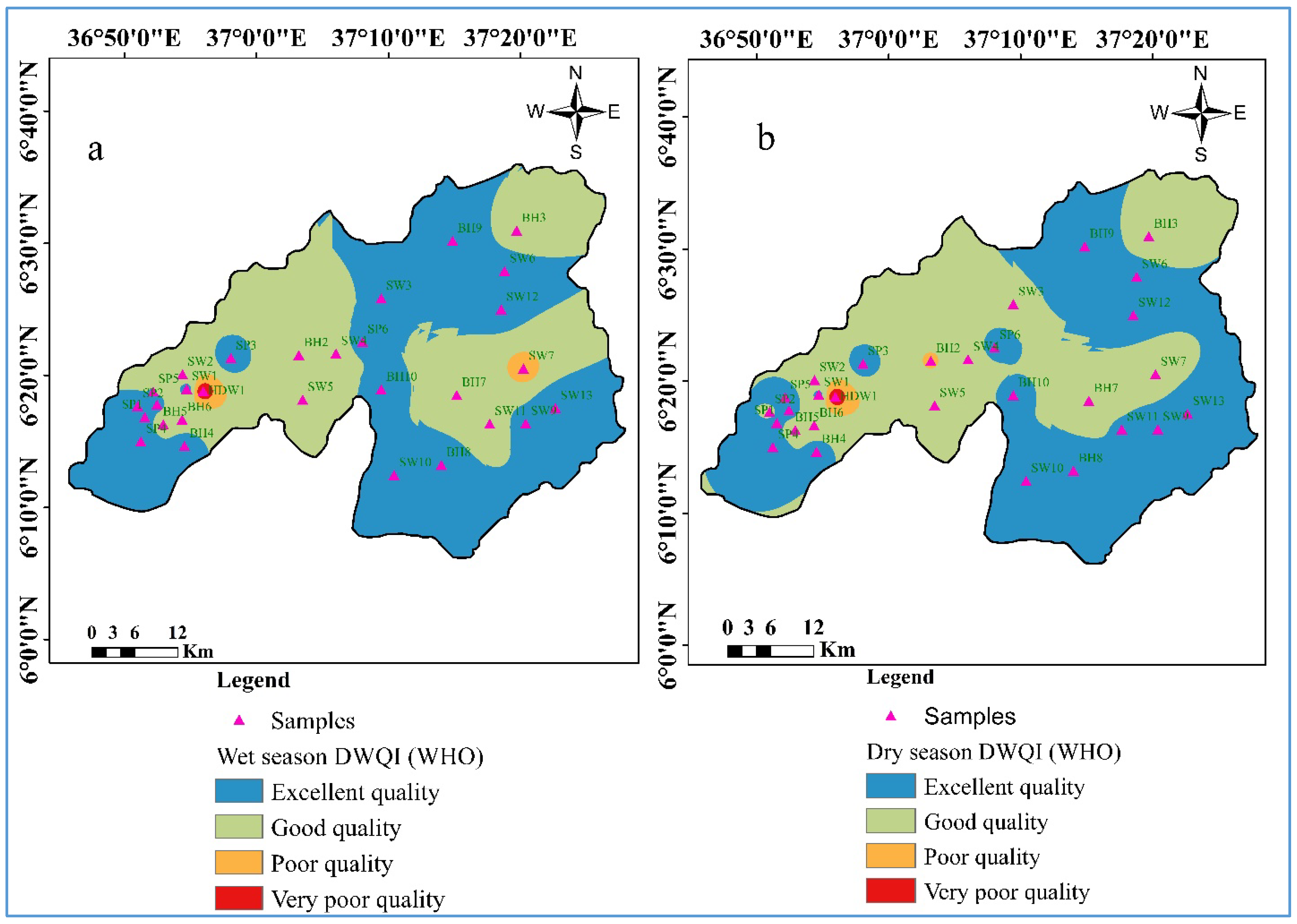
The water quality index (WQI) is a widely used method for assessing groundwater suitability by combining multiple physicochemical parameters into a single, easily interpretative value, reflecting both drinking and irrigation quality. First proposed by Horton [40] and refined through subsequent studies [41], the WQI has been applied under diverse hydrogeological conditions for water resource monitoring [37,42,43]. In this study, WQI was integrated with ArcGIS 10.8 to classify groundwater quality and compared against World Health Organization (WHO) water quality standards.

Seventeen key water quality parameters including pH, EC, TDS, temperature, major cations (Na⁺, K⁺, Ca²⁺, Mg²⁺, Fe²⁺) and anions (Cl⁻, F⁻, NO₃⁻, SO₄²⁻, CO₃²⁻, HCO₃⁻), along with alkalinity and total hardness were analyzed for their relevance to water chemistry, human health, and irrigation suitability [44]. The Water Quality Index (WQI) was computed through four main steps: parameter selection, weight assignment, quality rating calculation, and final index determination.

Each parameter was assigned a weight (w) from 1 to 5 based on its relative significance, with higher weights for parameters posing direct health risks, such as fluoride and nitrate [45,46,47]. These weights were standardized to relative weights (W_i) using the weighted arithmetic index method:

$$Wri={\displaystyle \frac{wi}{{\sum }_{i=1}^{n}wi}}$$

(2)

where Wri is the relative weight of the ith parameter, wi is the assigned weight of the ith parameter, and n is the total number of parameters. The quality rating (Q_i) for each parameter was calculated as a percentage of the detected concentration (C_i) relative to the corresponding WHO standard (S_i):

$$Qi={\displaystyle \frac{Ci}{Si}}\times 100$$

(3)

The sub-index (SI_i) was obtained by multiplying the relative weight by the quality rating:

$$\mathrm{S}\mathrm{I}\mathrm{i}=\mathrm{W}\mathrm{i}\times \mathrm{Q}$$

(4)

where SIi is the sub-index of the ith parameter, Wri is the relative weight of the ith parameter, and Qi is the quality rating of the ith parameter. Finally, the Water Quality Index (WQI) was calculated by summing all sub-indices:

$$DWQI={\sum }_{I=1}^{n}SIi$$

(5)

Assessing groundwater quality for irrigation is crucial, as its mineral composition influences soil structure, fertility, and crop productivity [20,48]. Elevated dissolved ion levels can impede soil stability and water infiltration by causing salinity, decreasing permeability, and accumulating sodium [28,49,50]. To evaluate these risks, indices such as sodium adsorption ratio, magnesium adsorption ratio, residual sodium carbonate, Kelly’s ratio, permeability index, and sodium percentage are commonly applied.

Table 2. Irrigation water quality (IWQ) parameters and equations.

IWQ Parameters	References
$\mathrm{S}\mathrm{A}\mathrm{R}={\displaystyle \frac{{\mathrm{N}\mathrm{a}}^{+}}{\frac{\sqrt{{\mathrm{C}\mathrm{a}}^{+2}+{\mathrm{M}\mathrm{g}}^{+2}}}{2}}}$	[51]
$\mathrm{M}\mathrm{A}\mathrm{R}={\displaystyle \frac{{\mathrm{M}\mathrm{g}}^{+2}}{{\mathrm{C}\mathrm{a}}^{+2}+{\mathrm{M}\mathrm{g}}^{+2}}}\times 100$	[52]
$Na\%={\displaystyle \frac{{Na}^{+}+K^{+}}{{Ca}^{+2}+{Mg}^{+2}+{Na}^{+}+K^{+}}}\times 100$	[53]
$RSC={(HCO}_3^{2-}+{CO}_3^{2-})-({Ca}^{+2}+{Mg}^{+2})$	[54]
$\mathrm{P}\mathrm{I}={\displaystyle \frac{{\mathrm{N}\mathrm{a}}^{+}+\sqrt{{\mathrm{H}\mathrm{C}\mathrm{O}3}^{-}}}{{\mathrm{C}\mathrm{a}}^{+2}+{\mathrm{M}\mathrm{g}}^{+2}+{\mathrm{N}\mathrm{a}}^{+}}}$$\times$100	[55]
$KR={\displaystyle \frac{Na+}{{Ca}^{+2}+{Mg}^{+2}}}$

presents formulas for all ion concentrations, which are reported in milliequivalents per liter (meq/L).

2.5. Entropy Weight Quality Index (EWQI)

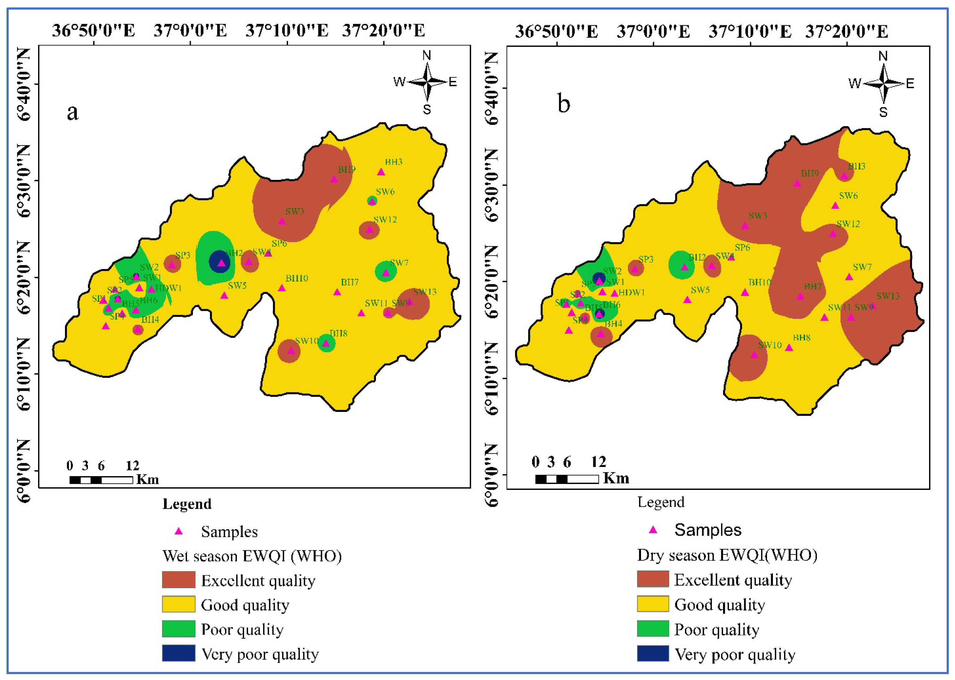
An entropy-based weighting scheme was used to assign objective weights to each physicochemical parameter and to aggregate them into the entropy-weighted water quality index (EWQI), a composite indicator of water quality. The computational workflow is described in the steps that follow [3,25,56].

Step 1. An entropy-based weighting approach was applied to the hydrochemical dataset consisting of m groundwater samples and n hydrochemical parameters [25]. In the first step, the data were arranged into the data matrix X, whose elements xij denote the value of parameter j measured in sample I (Equation (6)).

$$X=\left(\begin{array}{c}x11 x12 x13\dots \dots \dots \dots \dots \dots x1m\\ x21 x22 x23\dots \dots \dots \dots \dots \dots x2m\\ x31 x32 x33\dots \dots \dots \dots \dots \dots x3m \\ . \\ . \\ . \\ xn1 xn2 xn3\dots \dots \dots \dots \dots \dots xnm\end{array}\right)$$

(6)

where x11 is the value of the first parameter in the first sample, and general, xij is the measurement of the jth parameter in sample i. The entropy-weight calculation then proceeded from X by normalizing each column, computing the parameter-wise information entropy, and deriving objective weights for aggregation.

Step 2: The standardization process “yij” was evaluated, and then the standard evaluation matrix “Y” was obtained following Equations 7 and 8, respectively.

$$yij={\displaystyle \frac{xij-\left(xij\right)min}{\left(xij\right)\max -\left(xij\right)min}}$$

(7)

$$Y=\left(\begin{array}{c}y11 y12 y13\dots \dots \dots \dots \dots \dots y1m\\ y21 y22 y23\dots \dots \dots \dots \dots \dots y2m\\ y31 y32 y33\dots \dots \dots \dots \dots \dots y3m \\ . \\ . \\ . \\ yn1 yn2 yn3\dots \dots \dots \dots \dots \dots ynm\end{array}\right)$$

(8)

where xij is the initial matrix; (xij) min and (xij) max are the minimum and maximum values of the hydrochemical parameters of the samples, respectively.

The probability Pij corresponding to the normalized value yij of parameter j in sample i is defined as Equation (9):

$$Pij= {\displaystyle \frac{yij}{{\sum }_{i=1}^{m}yij}}$$

(9)

Step 3: The information entropy, ej, was computed by using Equation (10).

$$ej={\displaystyle \frac{1}{\ln m}}\sum _{i=1}^m(pij\times \ln pij)$$

(10)

After this, the entropy weight Wj was computed using Equation (11).

$$Wj={\displaystyle \frac{1-ej}{\sum _{i=1}^n(1-ej)}}$$

(11)

Step 4: The quality rating scale qj for every parameter was determined using Equation (12) as:

$$qj= {\displaystyle \frac{Ci}{Si}}$$

(12)

where Ci is the concentration in mg/L and Si permissible limit of [57] standard for each chemical parameter.

Step 5: The EWQI was calculated using Equation (13).

$$EWQI=\sum _{i=1}^{m}Wj\times qj$$

(13)

2.6. Pollution Index of Groundwater (PIG)

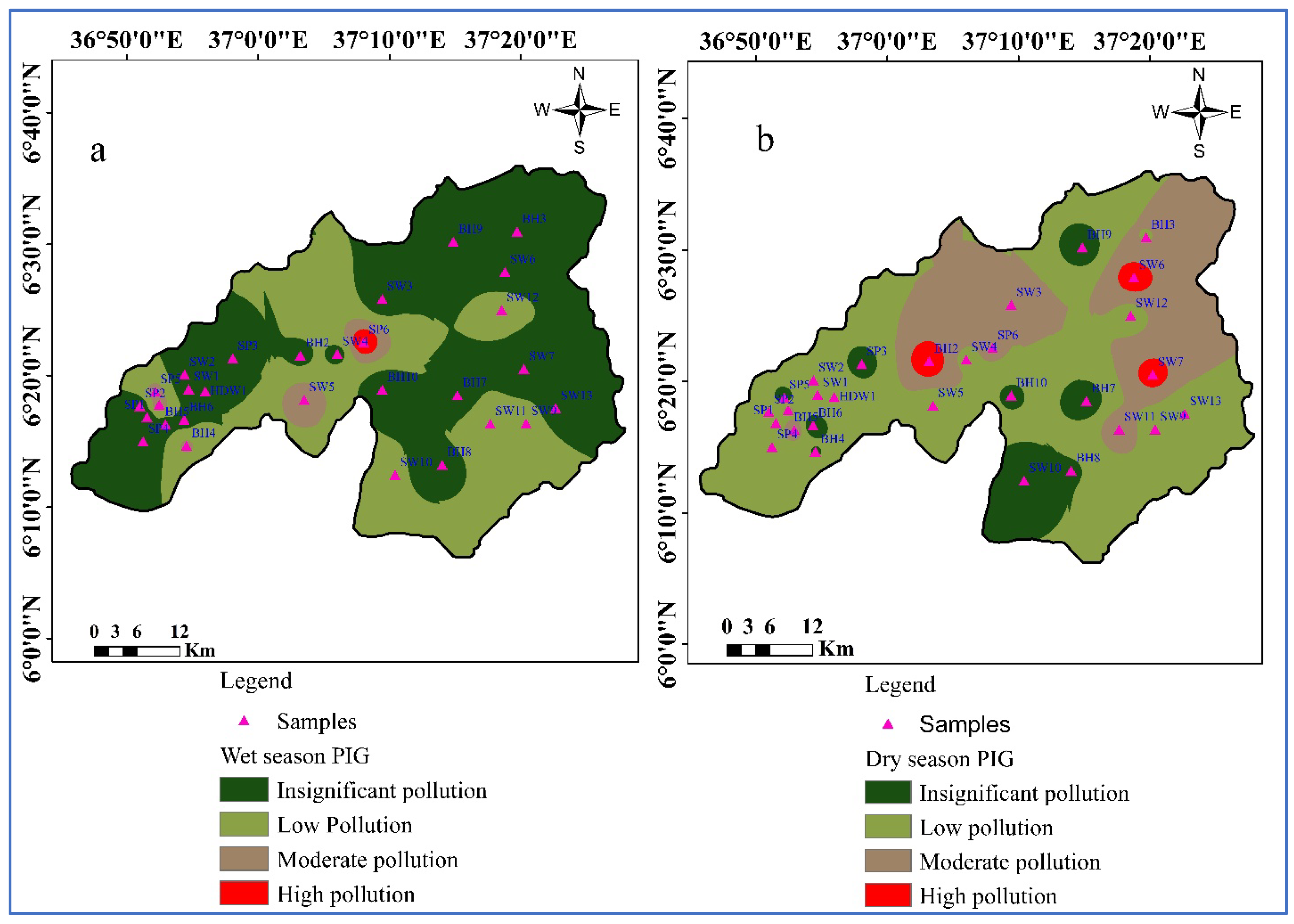
The Pollution Index of Groundwater (PIG) is a parameter-based scoring method used to assess overall drinking-water quality by combining the health-relevance of selected physicochemical variables (pH, EC, TDS, Ca²⁺, Mg²⁺, Na⁺, K⁺, Cl⁻, SO₄²⁻, NO₃⁻, HCO₃⁻, Fe²⁺, and F⁻). It translates measured concentrations into a single, interpretative index that highlights which sites and parameters drive contamination [58].

Step 1: Relative weight (RW)

In the Pollution Index of Groundwater (PIG) method, each water quality parameter was assigned a relative weight (RW) ranging from 1 to 5 based on its impact on human health. Parameters with the highest health significance, such as pH, TDS, SO₄²⁻, NO₃⁻, and F⁻, were assigned the maximum RW of 5, while Na⁺ and Cl⁻ were given a weight of 4, HCO₃⁻ a weight of 3, Ca²⁺ and Mg²⁺ a weight of 2, and K⁺ was given the minimum weight of 1. Thus, RW values reflect the relative importance of each parameter, with 1 indicating the least and 5 the most significant influence on human health [58,59].

Step 2: Parameter weight

Each water quality variable’s weight parameter (Wp) was calculated to determine its proportional contribution to overall groundwater quality. It was obtained by dividing a given parameter’s relative weight (RW) by the sum of RWs for all parameters, as expressed in Equation (14). This normalization ensures that the influence of each parameter on the Pollution Index of Groundwater (PIG) is relative to its assigned health significance, allowing balanced integration of all variables into the final index:

$$WP= {\displaystyle \frac{RW}{\sum RW}}$$

(14)

Step 3: The status of concentration (SC) for each water quality parameter was determined using Equation (15), where the measured concentration of a parameter in a water sample was divided by its corresponding WHO drinking water quality standard.

$$SC={\displaystyle \frac{C}{WHO}}$$

(15)

Step 4: The overall water quality was calculated using Equation (16).

$$OW=Wp\times SC$$

(16)

Step 5: The Pollution Index of Groundwater (PIG) was calculated by summing the overall weights (OW) contributed by each water quality parameter for a given sample, as shown in Equation (17).

$$PIG=\sum OW$$

(17)

2.7. Multivariate Statistical Approaches

Groundwater quality examinations often employ multivariate statistical analysis to identify contamination-related factors [3,56,58]. To show information most effectively, a variety of statistical methods are often used, usually with IBM SPSS 20 software. These methods include box-whisker plots, correlation coefficients, Gibbs plots, and principal component analysis (PCA). The correlation coefficient is a valuable tool for measuring the degree of dependence between variables. Examining correlations among water quality parameters can reveal significant hydrochemical relationships [59]. A correlation coefficient (r) of ±1 indicates a perfect linear relationship, whether positive or negative. Values closer to zero suggest a weak or negligible association between the variables. Values of r > 0.65 indicate strong correlations, and values between 0.5 and 0.65 reflect moderate correlations [56]. PCA primarily analyzes the variance within large datasets of interrelated variables by reducing them to a smaller set of independent components. These principal components provide detailed insights into the dataset’s most influential factors, thereby minimizing data complexity while preserving the essential information [60].

3. Results and Discussion

3.1. Groundwater Quality Parameters

The physicochemical properties of groundwater in the study area were evaluated compared to World Health Organization (WHO) guidelines for drinking water [33]. Seasonal variations were observed, reflecting natural hydrogeochemical processes. Groundwater temperature ranged from 20.4–25.3 °C (mean 22.3 °C) in the wet season and 22.8–27.3 °C (mean 24.6 °C) in the dry season, with higher temperatures in the latter due to reduced recharge and increased ambient temperature. pH values indicated predominantly alkaline conditions, ranging from 6.6–8.6 (mean 7.8) in the wet season and 6.8–8.8 (mean 7.9) in the dry season, showing a slight increase in alkalinity during the dry period likely caused by evaporation and ion concentration (Table 3).

Electrical conductivity (EC) varied from 161.2–733 µS/cm in the wet season (mean 450 µS/cm) and 201–916.3 µS/cm in the dry season (mean 554.1 µS/cm), reflecting increased ionic enrichment under dry conditions. Similarly, total dissolved solids (TDS) rose from 48.7–517 mg/L (mean 236.7 mg/L) to 60.9–646.6 mg/L (mean 296.7 mg/L), indicating enhanced mineralization from prolonged water–rock interaction. Alkalinity remained relatively stable in both seasons, ranging from 32.5–95.5 mg/L in the wet season and 28–82.2 mg/L in the dry season, while total hardness varied more widely, from 47.7–1067.7 mg/L in the wet season and 73.8–1212.1 mg/L in the dry season, reflecting consistent contributions of calcium and magnesium primarily from mineral dissolution. This seasonal increase is commonly attributed to reduced groundwater recharge, higher evaporation rates, and prolonged water–rock interaction during dry periods, which enhance dissolution of aquifer minerals and concentration of dissolved ions, as reported in previous studies [38,61].

Major ion chemistry of groundwater in the Maze Zenti catchment shows clear seasonal variability, largely controlled by hydrogeochemical processes and anthropogenic influences [4]. Calcium and magnesium concentrations were consistently higher during the dry season (15.4–198.7 mg/L and 8.6–174 mg/L, respectively) than in the wet season (12.8–189 mg/L and 3.8–145 mg/L), indicating intensified rock–water interaction and increased dissolution of carbonate and silicate minerals under reduced recharge and longer residence time, as also reported in similar groundwater systems [22,62]. Sodium (1.6–81.6 mg/L) and potassium (1.1–18.7 mg/L) remained low–moderate in both seasons, suggesting limited contribution from evaporite minerals and a dominant geogenic control.

Among anions, bicarbonate was the dominant species in both seasons, reflecting the prevalence of carbonate weathering processes, while sulfate and chloride occurred at lower concentrations, with a slight dry season increase likely linked to evaporative concentration. Nitrate exhibited high spatial and seasonal variability, occasionally exceeding the WHO guideline value of 50 mg/L during the wet season, which points to localized anthropogenic inputs such as agricultural runoff and surface-derived contamination mobilized during rainfall events [11,63]. Fluoride concentrations remained within permissible limits but showed higher dry season values (mean 1.6 mg/L) compared to the wet season (mean 0.9 mg/L), consistent with enhanced mineral dissolution under low recharge conditions. Iron also displayed a distinct seasonal contrast, increasing from 0.1 mg/L in the wet season to 0.2 mg/L in the dry season, reflecting geogenic contributions from aquifer materials and the influence of hydrological fluctuations, residence time, and redox conditions on iron mobilization within the groundwater system [24,64].

These findings are consistent with previous research. In the Upper Omo River Basin, Southern Ethiopia, Ref. [16] reported bicarbonate as the main anion year-round, with nitrate showing high spatial and seasonal variability that sometimes exceeded the WHO guideline. This was attributed to agricultural and surface-derived inputs, which aligns with the wet-season patterns observed in this study. Fluoride concentrations were slightly higher during the dry season in their study, and iron levels exhibited seasonal contrasts driven by geogenic sources and hydrological conditions, similar to the patterns seen here. Likewise, in South India, the authors of [29] found bicarbonate-dominated groundwater with minor contributions from sulfate and chloride. They also noted elevated nitrate levels in areas influenced by intensive agriculture, confirming that carbonate weathering, agricultural inputs, and aquifer geochemistry play significant roles in controlling the seasonal variability of groundwater chemistry.

Seasonal variation analysis using one-way ANOVA showed that temperature (T°C) was the only parameter with a statistically significant seasonal difference (F = 27.55; p < 0.05). Higher values were observed during the dry season, while all other parameters remained relatively stable.

Table 3. The descriptive statistical analysis of groundwater quality parameters in the study area.

Permissible Limit			Wet Season				Dry Season
Parameter	Ref. [57]	Minimum	Maximum	Mean	Std. Dev	Minimum	Maximum	Mean	Std. Dev
T	-	20.4	25.3	22.3	1.1	22.8	27.3	24.6	1.2
pH	6.5–8.5	6.5	8.6	7.7	0.4	6.8	8.8	7.9	0.4
EC	1500	161.2	733	450	163.6	201	916.3	554.1	196.1
TDS	1000	48.7	517	236.7	112.5	60.9	646.3	296.7	142
Na+	200	1.6	68	17.7	13.1	1.9	81.6	24.1	17.4
K+	12	1.1	15.6	4.6	2.9	1.4	18.7	5.7	3.4
Ca2+	75	12.8	189	57.2	49.7	15.4	198.7	68	51.3
Mg2+	50	3.8	145	48.8	36.6	8.6	174	48.8	43
HCO3−	120	39.6	116.5	85.4	19.9	34.1	100.2	73.5	20.3
Cl−	250	0	17	7.7	3.7	0	20.4	9.4	4.7
SO42−	250	64.3	432	167.8	105.8	77.1	476	98.3	120.4
NO3−	50	39.6	116.5	88.4	20.5	34.1	118.9	76.2	22
F−	1.5	0.4	1.6	0.9	0.4	0.3	1.4	1.6	0.5
CO32−	-	0	0	0.	0	0	0	0	0
Fe2+	0.3	0	0.1	0.1	0.1	0	0.2	0.2	0.2
TH	500	47.7	1067.2	343.8	274.3	73.8	1212.1	371.9	305.4
Alkalinity	500	32.5	95.4	70	16.3	28	82.2	60.3	16.6

Note: units in mg/L except for pH (unitless), EC (µS/cm) and T (°C); St. Dev stand for standard deviation and n = 30 groundwater samples, including 24 wells and 6 springs.

Table 3. The descriptive statistical analysis of groundwater quality parameters in the study area.

Permissible Limit			Wet Season				Dry Season
Parameter	Ref. [57]	Minimum	Maximum	Mean	Std. Dev	Minimum	Maximum	Mean	Std. Dev
T	-	20.4	25.3	22.3	1.1	22.8	27.3	24.6	1.2
pH	6.5–8.5	6.5	8.6	7.7	0.4	6.8	8.8	7.9	0.4
EC	1500	161.2	733	450	163.6	201	916.3	554.1	196.1
TDS	1000	48.7	517	236.7	112.5	60.9	646.3	296.7	142
Na+	200	1.6	68	17.7	13.1	1.9	81.6	24.1	17.4
K+	12	1.1	15.6	4.6	2.9	1.4	18.7	5.7	3.4
Ca2+	75	12.8	189	57.2	49.7	15.4	198.7	68	51.3
Mg2+	50	3.8	145	48.8	36.6	8.6	174	48.8	43
HCO3−	120	39.6	116.5	85.4	19.9	34.1	100.2	73.5	20.3
Cl−	250	0	17	7.7	3.7	0	20.4	9.4	4.7
SO42−	250	64.3	432	167.8	105.8	77.1	476	98.3	120.4
NO3−	50	39.6	116.5	88.4	20.5	34.1	118.9	76.2	22
F−	1.5	0.4	1.6	0.9	0.4	0.3	1.4	1.6	0.5
CO32−	-	0	0	0.	0	0	0	0	0
Fe2+	0.3	0	0.1	0.1	0.1	0	0.2	0.2	0.2
TH	500	47.7	1067.2	343.8	274.3	73.8	1212.1	371.9	305.4
Alkalinity	500	32.5	95.4	70	16.3	28	82.2	60.3	16.6

Note: units in mg/L except for pH (unitless), EC (µS/cm) and T (°C); St. Dev stand for standard deviation and n = 30 groundwater samples, including 24 wells and 6 springs.

3.2. Correlation Coefficient of Physiochemical Parameters

Pearson correlation analysis for the wet season (

Table 4. Correlation coefficient of chemical analysis for the wet season.

	pH	EC	TDS	Na+	K+	Ca2+	Mg2+	HCO3−	Cl−	SO42−	NO3−	F−	Fe2+
pH	1
EC	−0.52	1
TDS	−0.51	0.82	1
Na+	0.77	0.26	0.49	1
K+	0.18	0.03	0.24	0.02	1
Ca2+	0.68	0.30	0.42	0.50	−0.09	1
Mg2+	−0.24	0.71	0.33	0.65	−0.04	0.46	1
HCO3−	−0.20	0.39	0.13	−0.17	−0.31	0.16	0.04	1
Cl−	0.69	0.37	0.00	−0.11	−0.20	−0.10	0.02	0.19	1
SO42−	−0.21	0.28	−0.13	−0.09	−0.10	−0.12	0.05	0.36	0.18	1
NO3−	0.79	0.19	0.24	−0.07	0.21	−0.06	−0.06	−0.14	0.33	0.08	1
F−	−0.33	0.03	0.04	0.15	−0.15	0.02	0.11	−0.16	0.09	0.14	0.25	1
Fe2+	−0.17	0.04	0.22	0.09	0.07	0.11	0.32	−0.12	0.02	−0.19	0.42	0.17	1

Bold values indicate a strong correlation between physicochemical parameters.

) reveals that the dominant hydrogeochemical and anthropogenic processes controlling groundwater quality in the study area are in close agreement with findings from similar hydrogeological environments [3,25]. The strong positive correlation between electrical conductivity (EC) and total dissolved solids (TDS) (r = 0.82) confirms that groundwater conductivity is largely governed by dissolved ionic constituents derived from mineral dissolution and solute enrichment during recharge processes. This relationship is widely reported in groundwater systems where enhanced water–rock interaction and leaching of soluble salts play a key role in defining overall water chemistry [20].

In addition, the strong association between pH and nitrate (NO₃⁻; r = 0.79) suggests that nitrate enrichment is closely linked to alkalinity variations, reflecting the influence of agricultural activities, fertilizer leaching, and surface runoff during the wet season, as observed in intensively cultivated catchments [65]. Strong correlations of sodium (Na⁺) with TDS (r = 0.77) and calcium (Ca²⁺; r = 0.68) indicate the combined effects of silicate weathering, ion exchange, and partial carbonate dissolution during groundwater recharge, processes that have also been identified as key controls on groundwater chemistry in basaltic and mixed lithological terrains [28,33]. In contrast, the weak correlations of bicarbonate (HCO₃⁻) with most parameters suggest a relatively uniform distribution and a limited role in short-term water quality variation, whereas the strong correlation of chloride (Cl⁻; r = 0.69) points to localized anthropogenic inputs, particularly from sewage effluents and agricultural leachates. Overall, these correlation patterns emphasize the combined influence of geogenic processes and human activities on groundwater composition during the wet season, consistent with earlier regional and international studies [20,66].

These results are consistent with earlier study findings. Ref. [67] found high relationships between EC, TDS, and key ions including Na⁺ and Ca²⁺ in Tercha District, Dawuro Zone, Southern Ethiopia. These correlations reflect the combined effects of mineral weathering, carbonate dissolution, and anthropogenic inputs. Alkalinity and nitrate were also strongly correlated, indicating that agricultural runoff was a major factor. Similarly, Ref. [38] found significant correlations of Na⁺ and Ca²⁺ with TDS and a large positive connection between EC and TDS in Bougaa, Northeastern Algeria, indicating that ion exchange and water–rock interactions are important hydrogeochemical regulators. Both studies support the findings that groundwater composition during the wet season is shaped by the interplay of geogenic processes and human activities, demonstrating consistency across different lithological and climatic contexts.

During the dry season, Pearson correlation analysis (

Table 5. Correlation coefficient of chemical analysis for the dry season.

	pH	EC	TDS	Na+	K+	Ca+	Mg2+	HCO3−	Cl−	SO42−	NO3−	F−	Fe2+
pH	1
EC	−0.51	1
TDS	−0.50	0.91	1
Na+	−0.44	0.21	0.67	1
K+	0.17	0.01	0.24	0.00	1
Ca2+	−0.48	0.20	0.36	0.49	−0.14	1
Mg2+	−0.21	0.21	0.71	0.6	−0.04	0.39	1
HCO3−	−0.21	0.31	0.13	0.87	−0.31	0.18	0.14	1
Cl−	−0.16	0.07	0.14	−0.15	0.17	0.07	−0.12	0.08	1
SO42−	−0.19	0.25	0.73	−0.01	−0.41	−0.11	0.09	0.15	−0.31	1
NO3−	−0.21	0.16	0.14	−0.02	0.17	−0.10	−0.04	−0.18	0.09	0.05	1
F−	−0.24	0.04	0.05	0.13	−0.12	0.02	0.14	−0.29	−0.11	0.12	0.13	1
Fe2+	−0.11	0.08	0.18	0.02	0.16	0.08	0.18	−0.11	0.20	−0.20	0.12	0.14	1

Bold values indicate a strong correlation between physicochemical parameters.

) reveals strong hydrochemical linkages that emphasize the dominant role of geogenic processes in controlling groundwater quality [8,66]. The very strong correlation between electrical conductivity (EC) and total dissolved solids (TDS) (r = 0.91) confirms their common dependence on dissolved ionic concentration, reflecting intensified mineral dissolution under prolonged water–rock interaction during low recharge conditions. Strong positive correlations of sodium, magnesium, and sulfate with TDS (r = 0.67, 0.71, and 0.73, respectively), together with the notable Na⁺-Mg²⁺ association (r = 0.68), indicate the dominance of silicate weathering, particularly feldspar and mafic mineral alteration, a mechanism also highlighted by earlier studies in dry season groundwater systems [8,15]. In contrast, the weak correlations of nitrate (NO₃⁻) with most parameters suggest localized anthropogenic inputs, such as fertilizer leaching and domestic waste, rather than basin-wide geochemical control. Low–moderate associations involving fluoride and iron (F⁻–NO₃⁻, r = 0.25; Fe²⁺–Mg²⁺, r = 0.32) further point to site-specific geochemical processes, including fluorite dissolution and iron mobilization under reducing conditions, consistent with observations reported in previous investigations [12,68].

3.3. Principal Component Analysis (PCA)

Principal Component Analysis (PCA) is a multivariate statistical approach widely applied in hydrogeochemical studies to reduce a large dataset into a smaller number of factors while retaining most of the variability in the original data [3,20]. In this study, PCA was performed on thirty hydrochemical parameters (

Table 6. Principal component of groundwater characteristics in the study area.

Wet Season					Dry Season
Parameters	PC1	PC2	PC3	PC4	PC1	PC2	PC3	PC4
pH	−0.68	0.83	0.08	−0.11	−0.41	0.16	0.08	0.06
EC	0.77	0.14	−0.03	−0.36	0.63	0.68	0.04	−0.33
TDS	0.88	−0.36	−0.04	−0.37	0.74	−0.38	0.07	−0.24
Na+	0.83	−0.25	−0.23	0.62	0.73	−0.09	0.61	0.40
K+	−0.04	−0.30	0.72	−0.44	−0.04	−0.06	−0.05	−0.23
Ca2+	0.63	−0.15	−0.29	0.07	0.63	0.74	0.83	0.71
Mg2+	0.73	−0.13	−0.17	0.71	0.83	−0.25	0.11	0.83
HCO3−	0.09	0.73	−0.21	−0.23	0.08	0.32	0.72	−0.33
Cl−	0.14	0.36	0.63	0.01	0.05	0.73	0.11	0.01
SO42−	0.73	0.51	0.12	0.71	0.04	0.65	−0.27	0.73
NO3−	0.63	−0.01	0.56	−0.19	0.61	−0.15	−0.44	0.03
F−	0.15	−0.01	0.63	0.38	0.15	0.02	−0.49	0.63
Fe2+	0.15	−0.26	0.37	−0.04	0.18	−0.29	−0.24	−0.10
Eigen value	4.49	1.51	2.02	2.14	3.22	2.44	2.22	2.68
% of variance	34.57	11.63	15.56	16.49	24.73	18.73	17.11	20.63
Cumulative %	34.57	46.19	61.75	78.24	24.73	43.46	60.58	81.21

). Only components with eigenvalues greater than 1 were retained, and variables with absolute loadings ≥ 0.60 were considered significant in determining the predominant factors controlling groundwater chemistry [56].

Principal component analysis (PCA) revealed distinct seasonal controls on groundwater chemistry, with results comparable to those reported in similar hydrogeological settings [5,65]. During the wet season, four principal components accounted for 78.24% of the total variance in groundwater quality. PC1 (34.57%) was dominated by TDS, EC, Na⁺, Mg²⁺, NO₃⁻, and SO₄²⁻, indicating enhanced mineralization driven by silicate weathering and partial anthropogenic influence, particularly from nitrate inputs during recharge, consistent with observations by earlier studies [68]. PC2 (11.63%), characterized by strong loading of pH and HCO₃⁻, reflects carbonate weathering processes and dilution by fresh recharge water, a pattern commonly associated with rainy-season groundwater evolution [45]. PC3 (15.56%) showed significant contributions from K⁺, Cl⁻, F⁻, and NO₃⁻, suggesting mixed anthropogenic inputs from fertilizers and wastewater along with geogenic contributions from fluoride-bearing minerals, in agreement with findings reported in agricultural catchment [5,14]. PC4 (16.49%), dominated by Mg²⁺ and SO₄²⁻, is attributed to evaporite dissolution and the influence of Mg-rich lithology, which become more apparent during variable recharge conditions.

In the dry season, four principal components explained a higher proportion of the total variance (81.21%), indicating stronger geochemical control under reduced recharge conditions. PC1 (24.73%) represents the combined influence of mafic and felsic rock weathering with residual anthropogenic nitrate contributions, reflecting prolonged water–rock interaction during groundwater residence, as similarly noted by [56]. PC2 (18.73%) is associated with increased salinity and evaporite dissolution, likely enhanced by evaporation and concentration effects typical of dry periods [45]. PC3 (17.11%), dominated by carbonate-related ions, reflects carbonate weathering and ion-exchange processes, while PC4 (20.63%) highlights the role of fluoride-bearing minerals and evaporitic sources in controlling groundwater chemistry. Overall, the PCA results demonstrate that seasonal shifts in recharge conditions strongly influence the relative importance of geogenic and anthropogenic processes, in close agreement with previous hydrogeochemical studies [45,68].

3.4. Hydrochemical Facies and Evaluation of Groundwater

The geochemical evolution of groundwater in the study area was evaluated using major ions and hydrochemical facies identified through Piper diagrams [3,13,69]. The Piper plots for the wet and dry seasons (Figure 3) revealed six distinct water types: Ca-Mg-HCO₃, Na-K-HCO₃, Na-HCO₃, Ca-HCO₃, Na-K-HCO₃, and Ca-Na-HCO₃ (Figure 3). The dominant Ca-Mg-HCO₃ facies represents groundwater circulating through fractured basalt and pyroclastic formations in recharge zones, where limited water–rock interaction and short residence time yield slightly mineralized water.

The Ca-HCO₃ types indicate early-stage geochemical development associated with carbonate dissolution in spring and shallow wells. In contrast, Na-HCO₃ and Na-K-HCO₃ facies, mainly in western discharge areas, reflect advanced mineralization resulting from cation exchange and silicate weathering within weathered basalt and alluvial sediments. The transitional Ca-Na-HCO₃ facies mark intermediate stages along the flow path. Overall, the distribution of facies demonstrates that groundwater chemistry is primarily controlled by lithology, residence time, and water–rock interaction rather than seasonal variation.

This finding aligns with findings from [20] in the Jimma area of Ethiopia. They found that Na-HCO₃ types showed longer residence times and more intense water–rock interactions in volcanic terrains, while Ca-Mg-HCO₃ waters were linked to shallow aquifers and early-stage geochemical development. Similarly, Ref. [63] discovered that Ca-Mg-HCO₃ predominated in the recharge zones of the Hindon River Basin in India, while Na-HCO₃ facies took over in regions with longer flow pathways and worn lithologies. Similar patterns were found in the Ethiopian Rift’s Meki River Basin by [13], who emphasized the importance of lithology, residence time, and mineral dissolution in regulating groundwater facies. These consistent hydrochemical patterns demonstrate that the evolution of groundwater chemistry in a variety of volcanic and alluvial settings is dominated by geogenic processes rather than seasonal variation.

Box and Whisker plots (Figure 4) indicate that Ca²⁺, Na⁺, and Mg²⁺ are the major cations, while HCO₃⁻, SO₄²⁻, and Cl⁻ dominate the anions in the study area. Elevated Mg²⁺ and SiO₂ levels reflect silicate weathering of volcanic rocks, and the predominance of the weak acid anion HCO₃⁻ over stronger anions suggests active weathering in recharge zones. The lithology, dominated by basaltic and felsic volcanic rocks (Figure 2), strongly influences groundwater composition: Ca²⁺ is derived from amphibole, pyroxene, and feldspars; Mg²⁺ from olivine and clay minerals; and Na⁺ and K⁺ from feldspars and clays. These minerals contribute to groundwater chemistry through hydrolysis and weathering processes. The observed hydrochemical patterns align with trends reported in Ethiopian highland and rift valley aquifers, where silicate weathering, carbonate dissolution, and ion exchange govern groundwater composition [13,62,67,70] and are consistent with studies in similar volcanic terrains [10,16,30,71,72].

3.5. Groundwater Evaluation and Geochemical Signature

Groundwater chemistry in the Maze Zenti Catchment is primarily governed by geochemical reactions occurring as water interacts with the surrounding geological formations. The dissolution of minerals from basaltic and felsic volcanic rocks depends on their resistance to weathering and the degree of disequilibrium between infiltrating water and the host rock [13,48,73]. These water–rock interactions progressively mobilize ions such as Ca²⁺, Mg²⁺, and Na⁺, shaping the hydrochemical composition and providing insight into the mineralogical nature of the aquifer system [3,35,74,75].

The Gibbs diagram is a widely used tool for examining the relationship between aquifer lithology and groundwater chemistry [21]. It is divided into three major fields: precipitation dominance, rock–water interaction dominance, and evaporation dominance. In this study, the plotted data indicate that most groundwater samples have total dissolved solids (TDS) values ranging between 100 and 1000 mg/L. Furthermore, the ratios of Na⁺/(Na⁺ + Ca²⁺) and Cl⁻/(Cl⁻ + HCO₃⁻) predominantly fall within the range of 0 to 0.8. These distributions collectively suggest that rock–water interaction is the principal mechanism influencing groundwater chemistry in the study area, while the effects of precipitation and evaporation are relatively minor.

The Gibbs diagrams (Figure 5a,b) for the show that nearly all groundwater samples from the Maze Zenti catchment plot within the rock–water interaction dominance field. This pattern indicates that mineral dissolution processes, particularly involving silicate and carbonate weathering, are the primary controls on groundwater composition. Both the TDS versus Na⁺/(Na⁺ + Ca²⁺) and TDS versus Cl⁻/(Cl⁻ + HCO₃⁻) relationships further confirm that evaporation and precipitation exert limited influence, whereas silicate weathering and cation exchange govern solute acquisition. Most samples exhibit moderate TDS values and intermediate ionic ratios, reinforcing the conclusion that groundwater chemistry is largely shaped by natural water–rock interactions rather than by evaporation-crystallization processes. Although a few samples display slightly elevated sodium and chloride ratios, possibly reflecting minor ion-exchange effects, the overall geochemical evolution of groundwater in the catchment is predominantly controlled by aquifer mineral weathering and natural hydrogeochemical processes.

Prior research supports the findings of this study [39], the assessment of groundwater in Damot Gale Woreda, Wolaita Zone, Ethiopia, reported that groundwater chemistry is predominantly controlled by mineral dissolution processes, particularly silicate and carbonate weathering, with only limited influence from evaporation. Their observation of moderate TDS levels and dominant natural geochemical controls closely corresponds with the hydrochemical behavior identified in the Maze Zenti catchment. Similarly, in the Ambagarh Chowki region of Chhattisgarh, India, hydrogeochemical analysis indicated that groundwater chemistry is largely governed by rock–water interactions, especially silicate and carbonate weathering [68]. Interpretations from Gibbs and Piper diagrams showed that major ion patterns result primarily from natural mineral dissolution, with minimal contribution from evaporation or direct precipitation. Collectively, these studies reinforce the conclusion that, across both Ethiopian and Indian volcanic and basaltic terrains, rock–water interaction is the principal process controlling groundwater hydrochemistry, with secondary influences from anthropogenic or evaporative processes being limited.

3.6. Evaluation of Drinking Water Quality

3.6.1. Drinking Water Quality Index (DWQI)

Groundwater quality assessment is essential for safeguarding public health in the Maze Zenti catchment, where groundwater serves as the primary drinking source. In this study, field and laboratory analyses were conducted during both wet and dry seasons, evaluating water quality using the Drinking Water Quality Index (DWQI) based on 13 WHO-recommended parameters. The weighted index method reflects each parameter’s contribution to overall potability (

Table 7. The water quality index’s assigned weight and relative weight for the physicochemical parameters.

Parameter	Symbol	Unit	WHO Guideline	Weight (Wi)	Wri
pH	pH		6.5–8.5	4	0.08
Electrical Conductivity	EC	µS/cm	1500	3	0.06
Total Dissolved Solids	TDS	mg/L	1000	5	0.1
Sodium	Na+	mg/L	200	4	0.08
Potassium	K+	mg/L	12	2	0.04
Calcium	Ca2+	mg/L	75	4	0.08
Magnesium	Mg2+	mg/L	50	4	0.08
Bicarbonate	HCO3−	mg/L	120	2	0.06
Chloride	Cl−	mg/L	250	5	0.1
Sulfate	SO42−	mg/L	250	5	0.1
Nitrate	NO3−	mg/L	50	5	0.1
Fluoride	F−	mg/L	1.5	5	0.1
Iron	Fe2+	mg/L	0.3	3	0.06
Total sum				51	1

). Spatial DWQI maps (Figure 6a,b) indicate that most samples fall within the good-quality range (50–100), while excellent quality water (0–50) is concentrated in the southwest, south, southeast, northeast, and central zones. Slight seasonal variations were observed, whereas the southeastern and western region showed poor to very poor quality, likely due to agricultural runoff, lithological factors, and human activities. The results align with other Ethiopian studies, where volcanic and alluvial aquifers often yield good to excellent quality water [10,17,67,76]. However, the localized degradation in the southeast emphasizes the need for targeted management to address pollution sources. Geology, land use, and seasonal recharge are key drivers shaping the region’s groundwater quality patterns.

Groundwater quality in the Maze Zenti catchment was evaluated using the Drinking Water Quality Index (DWQI), which categorizes water as excellent, good, poor, very poor, for drinking. Analysis of 17 physicochemical parameters, thirteen of which were included in the DWQI calculation, revealed that no samples fell into the unsuitable category. During the wet season, 52.8% of the area exhibited excellent water quality, 45.8% good quality, and only 1.4% poor to very poor (

Table 8. Water quality classification based on DWQI and EWQI values for WHO standards.

WQI Value	Water Quality	Wet Season				Dry Season
		WHO Standard (DWQI)		WHO Standard (EWQI)		WHO Standard (DWQI)		WHO Standard (EWQI)
		Area (%)	Area (km2)	Area (%)	Area (km2)	Area (%)	Area (km2)	Area (%)	Area (km2)
0–50	Excellent	52.8	1235.8	13.1	306.2	51.6	1207.4	31.4	733.9
50–100	Good	45.8	1071.7	79.4	1858.4	47.4	1110.3	64.8	1518.4
100–200	Poor	1.2	28.8	6.8	159.2	0.8	18.4	3.5	79.3
200–300	Very poor	0.2	3.7	0.7	16.2	0.2	3.9	0.3	8.4
>300	Unsuitable	0	0	0	0	0	0	0	0
Total		100	2340	100	2340	100	2340	100	2340

). Dry season results showed slight improvement, with 51.6% excellent, 47.4% good, 0.8% poor, and 0.2% very poor. These seasonal variations reflect dilution and recharge effects, as precipitation enhances aquifer recharge and reduces ion concentrations, particularly in shallow, high-permeability aquifers [37,38,69].

These results are consistent with previous studies conducted in Ethiopia and other regions. According to [20], groundwater from Jimma’s volcanic terrains mostly meets WHO-recommended quality standards, with only a few remote exceptions linked to geogenic variables and human activities. Similarly, Ref. [13] observed that the majority of the groundwater in the Meki River Basin is suitable for drinking due to the lithology of the Rift Valley and agricultural activities, with occasional degradation in areas affected by human inputs. Ref. [63] also found that, while Na-rich and highly mineralized waters require close monitoring, Ca-Mg-HCO3-dominated waters in the Hindon River Basin, India, are generally safe to drink. Overall, these comparisons indicate that while volcanic and alluvial aquifers typically yield drinkable groundwater, localized degradation stemming from lithology, land use, and human activity necessitates targeted treatment to ensure sustained access to safe drinking water.

Seasonal variations indicate that both anthropogenic and geogenic factors influence groundwater quality. Agricultural runoff, inadequate sanitation, and mineral dissolution contribute to localized degradation, while rainfall recharge during the wet season dilutes ion concentrations. In the dry season, reduced flow and longer residence times promote mineral dissolution, increasing calcium, magnesium, sodium, and bicarbonate levels. Consequently, very poor quality areas account for 0.2% in the wet season and 0.8% in the dry season under WHO classification. The predominance of Ca-Mg-HCO₃ water reflects regional geochemistry, driven by carbonate weathering and silicate dissolution from gneiss and basaltic formations. Despite minor seasonal fluctuations, no water was classified as unsuitable, indicating that groundwater is generally safe for drinking, though continuous monitoring is advised to manage localized risks.

3.6.2. Entropy Weight Method

The entropy-weighted water quality index (EWQI), computed using Equations (6)–(13), provides an integrated assessment of drinking water suitability, with values above 100 indicating water unfit for consumption [59,77]. In the Maze Zenti catchment, EWQI shows clear spatial patterns with moderate seasonal variation. During the wet season, groundwater quality is predominantly good, covering about 79.4% of the area, while 13.1% is classified as excellent and only 7.5% falls into poor or very poor classes. In the dry season, excellent-quality zones expand to 31.4%, good-quality water remains dominant at 64.8% and poor and very poor areas contract to 3.5% and 0.3%, respectively, reflecting reduced leaching and diminished surface-runoff influence.

The spatial distribution of the EWQI in the Maze Zenti catchment (Figure 7a,b) reveals that groundwater quality is strongly influenced by lithology and the type of water source. Areas underlain by basaltic flows and ignimbrite units generally show higher EC, TDS, and major ion concentrations, resulting in relatively lower water-quality classes. This is attributed to longer groundwater residence times, intensive water–rock interaction, and the mineralogical composition of these volcanic rocks, which promote the dissolution of ions into the groundwater. Similarly, rhyolite and granite formations contribute to moderate variations in water quality due to slower recharge and moderate mineral content. In contrast, alluvial deposits, which are well connected to surface recharge and shallow springs, exhibit excellent to good water quality, reflecting lower residence times, dilution effects, and reduced water–rock interaction. Gneiss unit display localized variations, where shallow springs tend to have lower solute concentrations, but deeper wells intersecting mineral-rich zones show elevated EC, TDS, and minor ion enrichment. These lithological and hydrogeological controls explain the occurrence of poor water quality pockets in the northwest and central parts of the catchment, while most of the area maintains safe and favorable drinking water conditions. Variations among sampling points further emphasize the influence of source type, aquifer depth, and recharge dynamics on groundwater chemistry.

3.7. Pollution Index of Groundwater (PIG)

The Pollution Index of Groundwater (PIG) integrates multiple physicochemical parameters into a single value, providing a broad assessment of water quality and its suitability for drinking [59]. PIG is classified into five categories: insignificant (<1), low (1–1.5), moderate (1.5–2), high (2–2.5), and very high pollution (>2.5) [59,77], helping to identify areas with safe water and those at risk. In the Maze Zenti catchment, PIG values range from 0.13 (insignificant) to 2.13 (high). During the wet season (Figure 8a), most of the Maze Zenti catchment exhibits insignificant to moderate groundwater pollution, due to limited dilution and increased evaporation [58,59]. High-pollution zones occur in central and northeastern areas underlain by mafic-basaltic flows and granite, where prolonged water–rock interaction and nearby agricultural or settlement activities enhance mineralization. Groundwater in ignimbrite and rhyolite units shows moderate pollution, while wells in alluvial deposits have lower PIG values due to recharge and dilution. Gneiss and granitic areas show localized elevated PIG. These patterns indicate strong lithological and source control on water quality, requiring targeted management in high-risk zones.

During the dry season (Figure 8b), most of the Maze Zenti catchment shows insignificant to moderate groundwater pollution due to limited dilution and increased evaporation. High-pollution zones occur in central and northeastern areas underlain by mafic-basaltic flows where prolonged water–rock interaction enhances mineralization. Groundwater in ignimbrite and rhyolite units shows moderate pollution, while wells in alluvial deposits have lower PIG values due to recharge and dilution. Gneiss areas exhibit localized elevated PIG where shallow wells intersect mineral-rich zones. Overall, the PIG distribution aligns with DWQI and EWQI results, indicating safe water in most areas but requiring targeted management in high-risk zones.

3.8. Suitability of Groundwater for Irrigation

3.8.1. Sodium Percentage (Na%)

Sodium percentage (Na%) and permeability index (PI) are key indicators for evaluating groundwater suitability for irrigation, as excessive sodium can degrade soil structure, reduce hydraulic conductivity, and lower crop productivity [10,19,75]. In the Maze Zenti catchment, 50% of groundwater samples in the wet season fall within the excellent Na% class, 20% are good, and 10% permissible, indicating generally low sodicity hazards. During the dry season, excellent samples decrease to 60%, with 23.3% good and 16.7% permissible, highlighting potential localized sodicity risks (

Table 9. Classification of groundwater based on the IWQ parameters.

IWQ Parameters	Range	Classes	No of Samples (Wet Season)	%	No. of Samples (Dry Season)	%
SAR [51]	<10	Excellent	8	26.67	24	80
	10–18	Good	22	73.33	6	20
	18–26	Doubtful	0	0	0	0
	>26	Unsuitable	0	0	0	0
MAR [52]	>50	Suitable	23	76.67	23	76.67
	<50	Unsuitable	7	23.33	7	23.33
RSC [54]	<1.25	Safe	25	83.33	27	90
	1.25–2.5	Marginally safe	3	10	2	6.67
	>2.5	Unsuitable	2	6.67	1	3.33
Na% [53]	<20	Excellent	21	70	18	60
	20–40	Good	6	20	7	23.33
	40–60	Permissible	3	10	5	16.67
	60–80	Doubtful	0	0	0	0
	>80	Unsuitable	0	0	0	0
PI [55]	>75	Excellent	11	36.67	11	36.67
	25–75	Good	15	50	16	53.33
	<25	Unsuitable	4	13.33	3	10
KR	<1	Suitable	22	73.33	25	83.33
	>1	unsuitable	8	26.67	5	16.67

).

3.8.2. Permeability Index (PI)

PI results support overall irrigation suitability, with 36.67% of samples classified as excellent and 50% as good in the wet season. In the dry season, 36.67% remain excellent, 53.3% good, and 10% unsuitable (Table 8), likely due to elevated magnesium or bicarbonate levels that can limit soil permeability and root growth. These patterns align with similar hydrogeochemical conditions reported in Ethiopia’s Rift and Raya Valleys [13,28,78].

3.8.3. Magnesium Adsorption Ratio (MAR)

Magnesium Adsorption Ratio (MAR) are important indicators for assessing irrigation water quality, as excessive magnesium can harden soils, while high carbonate concentrations reduce soil permeability [10,42,79]. In the Maze Zenti catchment, 76.67% of groundwater samples in both wet and dry seasons exhibited MAR values above 50, indicating good suitability for irrigation (Table 9).

3.8.4. Sodium Adsorption Ratio (SAR)

The Sodium Adsorption Ratio (SAR) is a key indicator of irrigation water quality, reflecting potential sodicity and salinity hazards that can impact soil structure and crop growth [80,81]. In the Maze Zenti catchment, SAR values during wet and dry seasons ranged from 0.01 to 12 meq/L, all below the critical threshold of 18 meq/L. Approximately 93.3% of samples were classified as good (10–18 meq/L) and the remainder as excellent (<10 meq/L), indicating low sodicity risk. Wilcox diagram analysis (Figure 9) corroborates these findings, with 86.4% of samples falling in the C2S1 category (medium salinity, low sodium hazard), 9.1% in C1S1, and only 4.5% in S4, likely due to localized contamination. No samples were found in high salinity or sodicity classes (C3-C4, S2-S3), confirming that groundwater is generally suitable for irrigation across the catchment.

3.8.5. Residual Sodium Carbonate (RSC)

RSC values further reflect irrigation safety, with 83.3% of samples in the wet season and 90% in the dry season classified as safe (<1.25 meq/L). Only a small portion of samples fell into marginal or unsuitable categories, suggesting that alkalinity-related risks are limited across the catchment (Table 9).

3.8.6. Kelly’s Ratio (KR)

The Kelly Ratio (KR), defined as the ratio of sodium (Na⁺) to the sum of calcium (Ca²⁺) and magnesium (Mg²⁺), is a key indicator of groundwater suitability for irrigation. A KR value below 1 indicates acceptable water quality, whereas values above 1 suggest sodium dominance that can reduce soil permeability and induce alkalinity harmful to crops [43,82]. In the Maze Zenti catchment, 73.3% of groundwater samples during the wet season exhibited KR values below 1, while 26.67% exceeded this limit. In the dry season, 83.3% of samples were suitable and 16.67% unsuitable for irrigation (Table 9), indicating generally low sodium hazard with localized concerns. Elevated KR values likely result from sodium enrichment due to silicate weathering, evaporation, and cation exchange in clay-rich or weathered volcanic terrains [38,83]. These findings underscore the need for targeted monitoring and management in areas exhibiting higher KR values to ensure long-term irrigation sustainability.

As shown in Figure 9, the Wilcox diagram indicates that the majority of shallow well groundwater in the study area falls within S1-C2, corresponding to low sodium hazard and medium salinity, which is generally suitable for irrigation. However, one groundwater sample is classified in S4-C2, representing very high sodium hazard despite medium salinity, indicating potential risk for soil sodicity if used for irrigation without proper management. The observed variation can be attributed to local hydrogeochemical conditions, including water–rock interaction, evapotranspiration, and seasonal recharge dynamics. In the wet season, rapid recharge dilutes solutes and reduces sodium hazard, whereas in the dry season, evaporation and limited recharge concentrate sodium and total dissolved salts in certain localized zones. Overall, these results suggest that while the groundwater resource is largely suitable for irrigation, site-specific monitoring and management are essential to prevent soil degradation in areas influenced by high sodium hazard, reflecting the importance of integrating seasonal hydrogeochemistry and spatial variability in irrigation water quality assessment.

4. Conclusions

The hydrogeochemical evaluation of groundwater in the Maze Zenti catchment within the Omo River Basin reveals that natural geogenic processes primarily silicate and carbonate weathering predominantly control groundwater chemistry. These processes produce the dominant Ca-Mg-HCO₃ water type and reflect the influence of gneissic and basaltic formations that govern the hydrochemical evolution of the catchment.

Geochemical and statistical analyses, including Piper, Gibbs, Pearson correlation, and PCA, consistently demonstrate that rock–water interaction is the principal mechanism governing groundwater composition. However, localized Na-HCO₃ facies and elevated nitrate, chloride, potassium, and fluoride levels in some areas indicate anthropogenic impacts such as fertilizer use and sewage infiltration, particularly during the wet season.

Irrigation suitability assessments (Na%, SAR, PI, MAR, RSC, and KR) show that most groundwater samples are suitable for agricultural use, with low–moderate salinity and sodicity hazards. A few localized zones exhibit moderate risks associated with magnesium and bicarbonate enrichment, which may affect soil structure and permeability if unmanaged.

Overall, the groundwater in the Maze Zenti catchment is suitable for both drinking and irrigation, reflecting the dominance of natural hydrogeochemical processes. Nonetheless, localized contamination and agricultural inputs highlight the need for continuous monitoring, improved land-use management, and protection of recharge zones to sustain water quality and ensure long-term resource safety.