Abstract
Mesa de Los Santos is an elevated plateau of the Eastern Cordillera of Colombia bordered by escarpments, where groundwater resources are limited to the local recharge. The geological unit with the greatest hydrogeological potential is Los Santos Formation (Lower Cretaceous), which presents three members (Lower, Medium and Upper). Based on stratigraphic information and hydrogeological information, three aquifer systems were characterized in the Upper Member: The Shallow Aquifer System (SAS), the Upper Aquifer 1 (UA1), and Upper Aquifer 2 (UA2). The SAS comprises discontinuous aquifers with groundwater flowing very close to the surface, circulating through weathered and fractured levels. UA1 and UA2 contain groundwater flowing through fractures. Groundwater in UA1 circulates through the top of the Upper Member, is underlain by a predominantly muddy base and exhibits an E-W and NE-SW flow consistent with the dip of the layers and the main directions of fractures. UA2 groundwater flows through the base of the Upper Member and is limited by the impermeable Middle Member. Stable water isotopes (δ18O, δ2H) data show three behaviors: (i) large temporal variability indicating a rapid flow through fractures in the three aquifers, and through primary porosity mainly due to weathering in the SAS; (ii) slower flows, with low temporal variability, showing well-mixed water of meteoric origin in the SAS, UA1, and UA2; (iii) groundwater with signs of evaporation indicating the connection between wetlands and the SAS in some cases.
1. Introduction
Water resources are a ubiquitous element in the management and conservation of natural systems, playing a crucial and cross-cutting role that underpins community resilience [1]. Globally, more than two billion people live in water-stressed areas, where water demand surpasses the available supply [2]. Assessing groundwater availability in these regions holds significant potential for improving access to this vital resource, generating social, economic, and environmental benefits for communities [3]. However, inadequate groundwater management can lead to long-term depletion due to excessive extraction that outpaces natural recharge rates [3]. In this context, studying aquifer hydrodynamics is essential for the sustainable management of water resources.
The study of aquifers hosted in sedimentary rocks is of particular importance due to their role as major reservoirs of groundwater for domestic, agricultural, and industrial use [4]. Sandstone aquifers are of major hydrogeological importance due to their widespread distribution and their capacity to store and transmit significant volumes of groundwater. Their hydraulic properties are largely controlled by primary porosity and intergranular permeability, which may be enhanced or reduced depending on factors such as grain size, sorting, cementation, and diagenesis [5]. However, their heterogeneity, related to depositional environments and post-depositional processes, exerts a strong influence on recharge, flow dynamics, and water quality [4].
Sandstone aquifers are typically dominated by intergranular flow within porous media, although other types of flow pathways, such as flow through weathered layers or fractures, may also be relevant. The weathering process of sandstone can enhance its porosity and permeability; stable quartz grains preserve the framework structure of the rock, and a fraction of feldspars can be weathered to clay; however, the net effect on permeability depends on clay and cement formation that can locally reduce pore connectivity [6]. Weathering in the upper meters of exposed rocks favors the development of shallow aquifers with water tables close to the surface [7,8]. These aquifers may be floored by clay accumulations formed through feldspar hydrolysis and the subsequent downward migration and deposition of fine particles within the soil profile. In low-lying areas, this process may be complemented by fluvial erosion, allowing the deposition of fine particles at the bottom, thus forming the aquifer’s lower confining layer.
Depending on the specific climatic conditions of a region, significant thicknesses of weathered rock can develop, which may be related to the presence of vegetation and the formation of wetlands, which are key ecohydrological systems [9], and can be defined as topographic depressions with saturated or near-saturated soils for most of the year, supporting dense vegetation [10]. Groundwater and wetlands interact through recharge and discharge processes, which are influenced by the hydraulic conductivity of geological materials, land topography, and temporal climate variations [9,10,11]. Aquifers associated with wetlands are typically shallow and highly vulnerable to contamination due to their proximity to the soil-atmosphere interface, which is regulated by the thickness of the unsaturated zone [12]. Understanding the interaction between surface and groundwater flows that sustain wetlands, along with their relationship to climatic variables, is essential for comprehending the hydrodynamics of the system and promoting both sustainable use of water resources and the conservation of ecosystem services [11].
On the other hand, fractured sandstone aquifers exhibit distinct porosity and permeability properties, where the presence of fractures associated with geological faults, bedding planes, and discontinuity intersections can serve as preferential pathways for fluid flow and contaminants, controlling groundwater flow directions within regional systems [13,14,15,16,17]. The orientation of fractures, their spatial relationships, and kinematic indicators from fracture planes provide insights into the stress field responsible for their formation, as well as their potential to remain open depending on whether they are oriented perpendicular, oblique, or parallel to the maximum horizontal stress [18,19,20]. When transport occurs primarily through fractures, fluid velocities are significantly higher compared to an aquifer behaving as a porous medium [13,21].
This research aims to characterize the groundwater dynamics in Mesa de Los Santos, Santander, a wet climate area (receiving over 1000 mm of annual rainfall) that experiences drinking water shortages during dry seasons [22], which can last up to four months [23], leading to water stress affecting both the population and economic development. This scarcity is primarily due to the limited availability of surface water and the incomplete knowledge of groundwater resources. Wells and boreholes have been drilled, allowing the community to collect groundwater to meet its basic needs. Although groundwater is exploited in the region, there is no precise conceptual hydrogeological model available to enable environmental authorities to effectively manage this resource.
Conceptual hydrogeological models are hypothetical representations that qualitatively describe and synthesize the functioning of subsurface systems, primarily based on geological, geophysical, hydrogeochemical and isotopic information [24,25,26]. Stable isotopes of water allow for determining the relationship between aquifers and recharge zones, environmental climatic conditions at the time of water infiltration, and the dynamics of the water cycle in watersheds [27,28,29,30,31]. The objective of this study is to develop a conceptual hydrogeological model that describes the functioning and flow dynamics of groundwater in the Mesa de Los Santos. To achieve this, information from the physical model is integrated and related to the hydrodynamic model, considering the different types of aquifers identified. The physical model includes data on wet, weathered, and fractured zones, as well as the stratigraphy of the region. Meanwhile, the hydrodynamic model is evaluated based on the behavior of groundwater levels, recharge processes, and hydraulic properties of the aquifers. Additionally, data on physicochemical parameters and stable isotopes of water are incorporated to characterize the aquifers.
2. Description of the Study Area
2.1. Location and Climate of the Study Area
The Mesa de Los Santos is located in the department of Santander, west of the Eastern Cordillera of Colombia, between the Andean Foothills and the Middle Magdalena Valley (Figure 1). It has a population of approximately 18,000 inhabitants [32,33]. This area is a plateau surrounded by escarpments, with altitudes varying between 300 and 1800 masl [34]. Its natural boundaries are defined by the Los Montes stream to the north, the Manco River to the east, the Chicamocha River canyon to the east and south, and the Sogamoso River canyon to the southwest (Figure 1). The Los Santos Formation is the most extensively exposed geological unit in the Mesa de Los Santos, covering an area of 205 km2. This formation consists of three members (Lower, Middle, and Upper), with the Upper Member having the greatest hydrogeological potential [34]. The study focuses on the Upper Member, which crops out across a 158 km2 orographic domain that defines the spatial extent of the area analyzed.
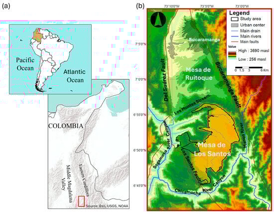
Figure 1.
(a) Regional location of the study area (red box), and (b) topographic elevation map, including main rivers, regional faults (red lines) and delineation of the Upper Member of the Los Santos Formation (black line).
The mesa is characterized by a natural slope from east to west of 2°. It has a flat morphology with gentle slopes of 0 to 4°, small hills in the central part with slopes of 4 to 8°, and terrain to the southwest with moderate slopes of 8 to 16° [34,35]. Towards the edges of the mesa, there are escarpments with steep slopes of 16 to 35° [35].
The climate in the study area follows a bimodal rainfall pattern, with two rainy seasons (April–May and September–October) and two dry seasons (June–July and December–January), following the zonal position of the Intertropical Convergence Zone [23]. A statistical analysis of days without rain shows dry periods that can last up to four months, mainly affecting the southwestern area. The average precipitation computed over a 20-year period and 10 stations across the area (1995–2014) results in a mean 1145.60 mm/year [36]. The data from the La Mesa-Station, operated by IDEAM (Instituto de Hidrología, Meteorología y Estudios Ambientales), shows a critical decline in rainfall in the southern part of the mesa over the past 45 years, with annual precipitations decreasing from 1008 mm/year (1974–1979) to 740 mm/year in the last decade (2010–2019), being likely an effect of climate change [23]. The uneven distribution of rainfall on the Mesa led to differences in vegetation cover between the southern and northern areas. In the northern region, there is a greater abundance of vegetation and the development of black soil rich in organic matter, especially in lowland areas, while the southern region is subjected to semi-arid conditions (Figure 2).
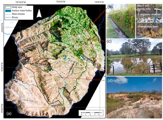
Figure 2.
(a) True-color satellite image showing vegetated areas (green) (https://browser.dataspace.copernicus.eu/ accessed on 20 December 2024). (b) Photographic record of black soils developed on altered rock in the humid, vegetated landscape. (c) Photographic record of a natural surface water body. (d) Photographic record of vegetation and bare soil in semiarid conditions prevailing in the southern part.
The average annual temperature is 22 °C, with a minimum daily average temperature of 17.6 °C in October and a maximum temperature of 28 °C in July and September. Garzón and Salcedo [37] estimated the potential recharge on a monthly scale using a SWB (soil water balance) code, for the period between October 2020 and September 2021, using data from the Llanadas Meteorological Station operated by GPH (Research Group on Water Resources). As a result, they obtained an annual precipitation of 948 mm/year, an actual evapotranspiration of 799 mm/year, a vegetation interception of 11 mm/year, a runoff of 4.2 mm/year, and a potential recharge of 133.8 mm/year. Figure 3 shows the behavior of precipitation and actual evapotranspiration during the analyzed period, as well as their relationship with the estimated potential recharge for each month. The behavior of actual evapotranspiration follows the same trend as precipitation. The months with higher precipitation (p) correspond to those with greater potential recharge (r): October 2020 (p = 143.36 mm, r = 28.95 mm), November 2020 (p = 114.76 mm, r = 28.75 mm), and June 2021 (p = 107.55 mm, r = 39.95 mm). In contrast, January 2021 recorded the lowest precipitation (p = 2.84 mm) and no potential recharge (r = 0.0 mm).
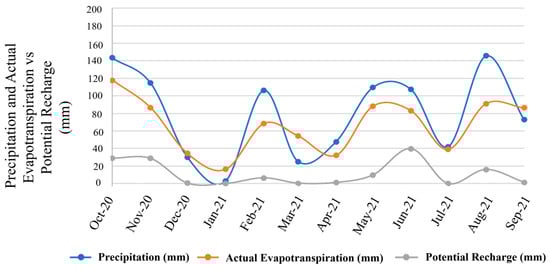
Figure 3.
Monthly behavior of precipitation, actual evapotranspiration, and potential recharge from October 2020 to September 2021.
2.2. Geological Framework
The Mesa de Los Santos is a structural mesa located in the Mesas y Cuestas region of the Eastern Cordillera, which was initially studied by Julivert [38], who defined the Bucaramanga-Ruitoque-Los Santos zone as a submerged block, limited by the Bucaramanga Fault to the east and the Suárez Fault to the west (Figure 1).
The region is characterized by a basement of Paleozoic metamorphic rocks and Jurassic igneous rocks on which sedimentary rocks of the Lower Jurassic and Lower Cretaceous were deposited and subsequently dip to the westward [39,40]. Pre-Cretaceous erosion beveled the Jurassic units for a later deposition of transgressive marine sediments towards the Santander Massif, forming an angular unconformity between the Jordán Formation (Lower Jurassic) and the Los Santos Formation (Lower Cretaceous), which is visible in some areas of the escarpments of the Mesa de Los Santos [41,42,43,44]. The elevated blocks that make up the Mesas y Cuestas region are bordered by a highly evolved hydrographic network [39], which forms deep canyons (e.g., Chicamocha River and Sogamoso River canyons, Figure 1).
2.2.1. Lithostratigraphic Framework
In the Mesa de Los Santos, the crystalline basement consists primarily of Paleozoic metamorphic rocks of the Silgará Schists. These have been intruded by the Jurassic Pescadero Granite [39,40]. The sedimentary sequence from base to top corresponds to: reddish brown to violet claystone interbedded with fine-grained sandstone of the Jordán Formation of Lower Jurassic age [34,42,43,44]; Lower Cretaceous strata correspond to (i) conglomerates, conglomeratic sandstone, siltstone and quartz sandstone of the Los Santos Formation, (ii) limestone of the Rosa Blanca Formation, (iii) gypsum lutite and limestone of the Paja Formation, and (iv) limestone of the Tablazo Formation [34,39,40] (Figure 4). Los Santos Formation, which constitutes the geological unit object of the present study, outcrops over most of the surface of the Mesa de Los Santos and its thickness increases from the eastern edge to the western edge of the Mesa, varying in thickness between 120 and more than 200 m [39].
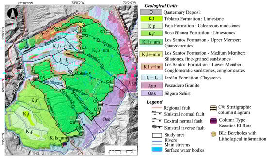
Figure 4.
Geological map of the study area (Modified from García-Arias et al. [45]).
Langenheim [46] was the first to establish that Los Santos Formation in Mesa de Los Santos area is composed of three distinct members: a basal conglomerate member (Lower Member), an intermediate member consisting of gray sandstone interbedded with red shale or siltstone (Middle Member), and an upper sandstone member that forms cliffs (Upper Member). This subdivision was also adopted by Julivert et al. [39], Pinto et al. [47], Ingeominas [48], Díaz et al. [34], among other authors. However, Laverde [42,44] divided the unit into four segments: A, B, C, and D, where segment A corresponds to the Lower Member, segment B to the Middle Member, and segments C and D to the Upper Member [44]. The main lithological characteristics, sedimentary environments, and the proposed hydrogeological units for each member/segment are shown in Figure 5.
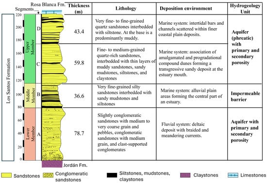
Figure 5.
Stratigraphic column of the El Roto type section (taken and modified from Laverde [41]), lithology and depositional environments of the Los Santos Formation segments [43], and hydrogeological unit [33,46].
2.2.2. Structural Framework
The structural framework of the Mesa de Los Santos is defined by two major regional structures: the Bucaramanga Fault to the east and the Suárez Fault to the west, along with a minor structure, the Los Montes Fault, to the north [45] (Figure 1). The Bucaramanga Fault is a sinistral transtensional fault with a significant vertical component [49], while the Suárez Fault is a reverse-sinistral fault with neotectonic activity [50], and the Los Montes Fault is a dextral transtensional structure that marks the northern boundary of the study area [45].
In the Mesa de Los Santos, the presence of joints and faults can facilitate the infiltration, circulation and recharge of aquifers [34]. The fracture systems have been studied by various authors [34,45,47], with the most recent study providing a kinematic interpretation of geological faults and establishing the main stress tensors and fracture patterns.
In the study area, normal faults with dextral and sinistral strike-slip movements, and reverse faults with sinistral strike-slip movements, are observed. (Figure 4). The kinematics of these faults are associated with NW-SE strike-slip stress tensors, varying from 105 to 156°, with a general maximum horizontal tensor (SHmax) of 111°, nearly parallel to most of the major faults in Mesa de Los Santos (Figure 4) [45].
The Mesa de Los Santos exhibits three predominant structural trends: SE-NW, SW-NE, and E-W, corresponding to the mapped faults in the region [47]. Among these, the SE-NW Los Santos Fault stands out. This structure extends beyond the study area to the north and south and separates the sandstones of the Los Santos Formation from the limestones of the Rosa Blanca Formation [45]. Therefore, this structure defines the southwestern boundary of the study area in this research. It is worth mentioning that some relict outcrops of the Rosa Blanca Formation are located to the northeast of the Los Santos Fault.
2.3. Hydrogeological Framework
Pinto et al. [47] and Díaz et al. [34] qualitatively assessed the porosity and permeability of Jordán, Los Santos, and Rosa Blanca formations. According to their conclusions, the Jordán Formation has low primary porosity and high fracture density, which could allow a flow transit but limited storage. However, given that the Jordán formation is predominantly composed of claystone, it is considered in the present study as the general hydrogeological basement, along with the Silgará Schists and Pescadero Granite.
The conglomerate and quartz sandstone constituting the Lower Member (segment A, 56 to 152 m thick) display high primary porosity and medium to high permeability, with high fracture density, forming a fractured aquifer [34,47]. In contrast, the siltstone, claystone, and sandstone of the Middle Member (segment B, 22 to 41 m thick) have low porosity and permeability, acting as an impermeable barrier with no significant hydrogeological potential [34,47].
The Upper Member (segments C and D, 33 to 95 m thick) is considered the geological unit with the highest hydrogeological potential, composed mainly of fine-grained sandstone [34]. In the northern zone, the sandstone has a clayey-sandy matrix that slightly reduces rock permeability, with a primary porosity between 6 and 8%. To the east and west, the sandstones contain a high percentage of siliceous cement, presenting medium permeability and medium secondary porosity associated with fracturing [34]. In the southern zone, a high density of fracturing is observed. Casadiegos et al. [51] reported two distinct aquifers within the Upper Member referred to as Shallow Aquifer and Upper Aquifer. The Shallow Aquifer is a phreatic aquifer related to quartz sandstone weathering profiles [51], located in depression areas and limited by clay accumulations due to feldspar hydrolysis. The Upper Aquifer is a fractured aquifer composed of well-cemented quartz–sandstones (siliceous cement), with low primary porosity [51].
Outcropping mainly southwest of the Los Santos fault, the Rosa Blanca Formation is predominantly composed of calcareous mudstones, limestones, and sandstone, with an estimated thickness of 300 m [47]. The top of the formation presents fractured and weathered rocks with the development of secondary porosity [47] and medium permeability [34]. The base and middle part of the formation may present secondary porosity due to fracturing but without significant karstification processes [47,48], resulting in low porosity and permeability [34]. This unit has a drilled well 215 m deep and a groundwater depth of 142 m, suggesting the existence of aquifers. However, the existence of exploitable water storage has not yet been clearly established and requires further study. Furthermore, a possible north–south water flow from the Lower Member of the Los Santos Formation to the Rosa Blanca Formation can be hypothesized.
3. Materials and Methods
An integrated approach was used to analyze the hydrodynamics of the aquifers present in the Los Santos Formation. This approach was based on the analysis of the physical model, piezometric levels, hydraulic parameters, and the behavior of the physicochemical parameters and the composition of stable isotopes in the groundwater.
3.1. Geological 3D Model
The inputs used for constructing the physical model include a 1:25,000 scale geological map, fracture patterns, nine stratigraphic column diagrams, a digital elevation model, and geological cross-sections. The geological map is obtained from Pinto et al. [47], modified by García-Arias et al. [45]. This map delineates the three members of the Los Santos Formation and defines the kinematics of the main structural features (Figure 4). The characterization of the fractures was based on the results obtained by García-Arias et al. [45]. The stratigraphic information includes field surveys conducted using Unmanned Aerial Vehicles (UAVs), which enabled the generation of Digital Outcrop Models (DOMs) at nine locations within the study area (Figure 4—points marked as C#). These sites corresponded to steep escarpments difficult to access, where UAVs proved essential for acquiring stratigraphic data.
The data obtained from UAVs were processed using Agisoft Metashape Professional (version 2.0.2) to generate DOMs. Using the software’s tools, the heights of stratigraphic contacts and apparent thickness of the layers were determined. It is worth noting that, since the layer inclinations are less than 10°, the thickness measurement error is negligible. For the remote identification of lithologies observed in the DOMs, a detailed textural analysis was performed, guided by the stratigraphic column directly recorded in the field at C7 (Figure 4). This classification broadly categorizes the textures into sandstone, mudstone, and conglomerate. The stratigraphic diagrams were digitized using Strater 5 (version 5.10.xxx), to identify the Lower, Middle, and Upper members of the formation, taking the previous studies [39,44,46,47,48] as a methodological guide for correlation and lithological description. The new field measurements allowed a more precise estimation of the thickness of each member.
Based on the digital elevation model (DEM), the geological map, stratigraphic columns, geological cross-sections, and available borehole data, a 3D model of the Los Santos Formation was constructed. The input dataset included the spatial coordinates of stratigraphic contacts, dip measurements, and fault traces, which defined the geological interfaces and structural framework of the area. The model was developed using the open-source Gempy library (version 3.2.2) implemented in Python, which applies implicit geological modeling through cokriging interpolation to generate continuous 3D surfaces between data points. Once the geological surfaces were generated, they were exported into the software Blender (version 4.1.0) using a Python script, where thicknesses were assigned to each geological unit and the digital elevation model (DEM) integrated for topographic consistency. The contact between the Middle Member and the Upper Member was used as a reference level for the modeling process. Subsequently, using the 3D geological model and the piezometric lines of the identified aquifers, the rock volumes corresponding to each aquifer were calculated, considering the separation of segments C and D within the Los Santos Formation and the contact with the Middle Member. The computed aquifer volumes allowed the estimation of groundwater reserves, providing valuable information for the integrated management of water resources in the study area.
3.2. Hydrodynamic Model
During 2020 and 2021, field visits were conducted to identify accessible groundwater points for the study. In total, 55 groundwater points were inventoried: 33 wells, 7 springs, 14 boreholes, and 1 piezometer. Each of these points was characterized by the height of the well mouths or the elevation of the springs measured using a Differential GPS (DGPS), as well as by the basic physicochemical parameters (temperature, pH, and electrical conductivity) and piezometric levels, when possible. After the inventory, periodic visits were conducted in 2021, 2022, and 2023 to collect data on the water table level and physicochemical parameters. Measurements of the water table level were obtained from 35 points (496 individual measurements in total), for which the minimum, maximum, and average values were determined. Using the k-means clustering algorithm in R-studio (version 2022.12.0), the levels were statistically classified and grouped. The integration of water table levels and field observations enabled the identification of the aquifers present in the Upper Member and allowed for a more precise delineation of the piezometric contours, from which a regional flow pattern was identified. The piezometric contour map was generated using the kriging interpolation method with an exponential semivariogram in ArcGIS Desktop 10.3.1 (ArpMap, Esri). The interpolation was based on the average piezometric values obtained from field measurements. Because the distribution of control points was limited, the kriging process included an extrapolation step to extend the processing to the entire study area. A spatial coverage analysis was then performed to distinguish zones with higher confidence (those located closer to the measurement points) from peripheral areas affected by higher uncertainty due to extrapolation. The kriging approach minimizes estimation variance, thus reducing potential interpolation errors and enhancing the reliability of the final piezometric map. The resulting contours were validated considering the topographic gradients and the location of the springs, which indicate groundwater discharge zones.
Each aquifer was characterized by information on physicochemical parameters and hydraulic parameters. The hydraulic parameters were determined by 14 pumping tests (one was conducted by the research team and the others by the environmental authorities).
Finally, the analysis of the dynamic behavior of stable water isotopes (δ18O, δ2H) in groundwater was assessed on samples collected between 2020 and 2022. Part of these data were previously presented in Cetina et al. [52], which included data from 2020–2021 groundwater and precipitation samplings. In the present study, the isotopic dataset was updated by incorporating additional groundwater data collected in 2022 (256 samples), allowing for a more comprehensive interpretation. The updated analysis is integrated with the results of the physical model and the identification of the different aquifers present in the Upper Member.
4. Results and Discussion
4.1. Geological Model
4.1.1. Lithological Observations
The digital outcrop models (DOMs) generated from UAV flights allowed for the identification of the predominant lithologies of the Los Santos Formation (Figure 6). To characterize the lithology from remote data, a textural interpretation of each layer observed in the DOMs was performed, using the stratigraphic column directly surveyed in the field at point C7 as a reference.
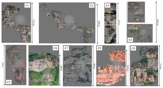
Figure 6.
Digital Outcrop Models generated from the escarpments of the Mesa de Los Santos. C#: Columns.
The outcrop at column C7 is accessible through the via ferrata “La Pared” climbing park, which facilitated the direct collection of geological information from the rock. Column C7 shows the following features from base to top:
- Lower Member (>6 m, segment A): thick fractured layers of light purple fractured sandy conglomerate. It contains subangular gravel with sizes ranging from granules to cobbles (2 to 55 mm), embedded in a medium-grained sand matrix. Compositionally, the gravel consists of quartz, sedimentary lithic fragments, potassium feldspar, and black lithics, with mica as an accessory mineral. The grain size of the rock matrix suggests high primary porosity and permeability, giving the Lower Member good potential for groundwater storage and transport through rock pores and fractures.
- Middle Member (51 m, segment B): a sequence of thin to medium tabular layers with irregular, well-defined contacts, composed of very fine to very coarse-grained sandstone with color variations ranging from violet to light gray and, to a lesser extent, light green. These sandstones are interbedded with medium to very thick layers of siltstone and mudstone in violet and green shades, containing muscovite. The sandstone grains are subrounded to subangular and are composed of quartz, black lithics, iron oxides, glauconite, plagioclase, and potassium feldspar, with a siliceous cement. Compositionally, the sandstones are classified as quartz arenites to sublitharenites. These layers exhibit very low primary porosity and no permeability, acting as a seal that separates the aquifers of the Upper Member and the Lower Member.
- Upper Member (90 m, segments C and D): a sequence of thick to medium tabular and wedge-shaped fractured layers with well-defined planar contacts. These layers consist of fine- to coarse-grained sandstone with colors ranging from light gray to yellowish-gray and orange-gray. The grains are subangular to subrounded and exhibit saturated contacts with siliceous cement precipitation, reducing the primary porosity, highlighting the importance of secondary porosity associated with fractures, in the storage and flow of groundwater present in the Upper Member. Compositionally, the sandstones contain between 80% and 95% quartz, along with black lithics, iron, manganese, and copper oxides, and traces of muscovite. The sandstones are classified as quartz arenites to sublitharenites. Toward the middle and top of the member, violet-colored mudstone layers are observed, separating segment C from D, allowing the description of two different aquifers. It is worth mentioning that this layer is not recorded in all columns.
Column C7 is a guide for a general classification of textures in sandstones, mudstones, and conglomerates from the layers observed in the DOMs. A total of 9 column diagrams were obtained (Figure 7). This approach provided stratigraphic information on the escarpments of the Mesa de Los Santos, enabling the identification of thickness variations in the members (Table 1).
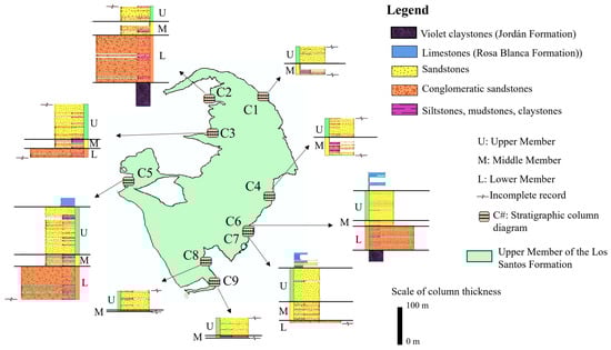
Figure 7.
Diagrams of stratigraphic columns distributed in the study area.
4.1.2. Geometry of the Strata
Based on the stratigraphic columns, lateral continuity of the three members was identified throughout the study area. The extensional tectonic regime during the Cretaceous, associated with the activity of normal faults (Bucaramanga, Suárez, Los Santos, and Los Montes faults [44,53,54], generated the accommodation spaces that made possible the lateral continuity of the units.
Columns C5, C6, and C7 contain the complete record of the Upper Member, as they show contact with relics of the overlying unit, the Rosa Blanca Formation, and with the underlying unit, the Middle Member. Likewise, columns C2 and C6 may record the full thickness of the Lower Member, as they present contact with the underlying unit, the Jordán Formation (Figure 7).
The Lower Member shows an apparent increase in thickness from east to west, as recorded in column C6 to the east (66 m) and column C2 to the west (126 m). Similarly, the Upper Member presents complete records in the east, with thicknesses of 79 m in column C6 and 70 m in column C7, while in the west, column C5 reaches 125 m (Table 1). These records align with the findings of Julivert et al. [39], who reported a general thickening of the entire unit from east to west. Additionally, erosion processes have affected the thickness of the Upper Member, leading to significant reductions in columns C1 (45 m), C2 (41 m), C4 (43 m), C8 (52 m), and C9 (46 m).

Table 1.
Thicknesses of the members and segments of the Los Santos Formation.
Table 1.
Thicknesses of the members and segments of the Los Santos Formation.
| Los Santos Formation | Columns | C1 | C2 | C3 | C4 | C5 | C6 | C7 | C8 | C9 | El Roto [42] | |
| Surface elevation (masl) | 1691 | 1470 | 1605 | 1772 | 1002 | 1742 | 1742 | 1618 | 1529 | 1113 | ||
| Member | Segment | Column Thicknesses (m) | ||||||||||
| Upper | D | 45 | 41 | 60 | 43 | 38 * | 53 * | 38 * | 52 | 46 | 43.4 * | |
| C | 30 | 87 | 26 | 52 | 59.8 | |||||||
| Middle | B | 31 | 38 | 29 | 57 | 34 | 14 | 51 | 3 | 6 | 36.6 | |
| Lower | A | 126 * | 24 | 90 | 66 * | 6 | 78.7 | |||||
| TOTAL | 76 | 205 | 143 | 100 | 249 | 159 * | 147 | 55 | 52 | 218.5 * | ||
* Complete record.
The Middle Member presents thick layers of siltstone and mudstone, where hydraulic conductivity (K) ranges from 10–0 to 10–12 (m/s), indicating low permeability [55], consistent with previous findings by Pinto et al. [47] and Díaz et al. [34]. This observation is consistent with the hypothesis of a hydraulic disconnection between the Upper and Lower Members.
Focusing on the Upper Member, the stratigraphy shows clay levels at different depths. The basal level present in the so-called segment D stands out. This level is observed only in columns C3, C5, C6, and C7, indicating lateral facies changes that may either disconnect or connect the water levels identified in the Upper Member. Based on this, two hypotheses are proposed: (i) two distinct aquifers are present in the segments C and D in the Upper Member, or (ii) a multilayer aquifer exists throughout the entire thickness of the Upper Member. To determine which model more accurately describes the hydrodynamic reality of the water, the results of the 3D physical model are integrated with piezometric levels, hydraulic parameters, physicochemical properties, and the isotopic composition of the water.
4.1.3. Three-Dimensional Model
Based on the stratigraphic information, a 3D model was generated using the Gempy modeling program and its graphic output was produced in the Blender program (Figure 8). This model shows the extension of the three members of the Los Santos Formation and their variations in thickness from east to west. The model output is consistent with previous work [34,47], confirming the presence of at least two aquifer systems: (i) the Lower Aquifer (conglomeratic sandstone of the Lower Member) and the Upper Aquifer System (quartz sandstone of the Upper Member) which will be detailed in the following section. The aquifer of the Lower Member mainly presents primary porosity and potentially secondary porosity due to fractures. It is defined as a captive aquifer, bordered at the top by the Middle Member and at the bottom by the Jordán Formation. This aquifer offers limited accessibility through extraction points; therefore, its hydraulic characteristics cannot be accurately defined. However, it may have an important hydrogeological potential for exploitation according to its lithological characteristics.
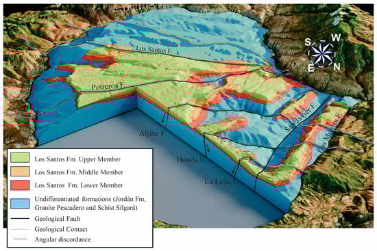
Figure 8.
Three-dimensional geological model of the Los Santos Formation in Mesa de Los Santos.
Geological faults are observed to cut across all geological units, suggesting that one of the main aquifer recharge processes of the lower units may occur through the vertical connection of faults and fractures, as proposed by García-Arias et al. [45] and Pinto et al. [47]. It is suggested that the infiltration process occurs from the surface to depths of 50 to 200 m (variation in the thickness of the Los Santos Formation). Normal faults such as Lejía, Honda and Aljibe present the same direction of SHmax tensor of 111°, favoring a flow of water through open fractures towards the NW as mentioned by García-Arias et al. [45].
4.2. Hydrodynamic Model
The groundwater points inventoried in the study area and the type of information provided at each point are included in Figure 9. These points only capture water from the Upper Member of the Los Santos Formation. Of the 55 evaluated points, 35 have piezometric level data, and 49 have records of physicochemical parameter and stable isotope data. The points where it was not possible to measure the physicochemical parameters correspond to those without a pumping system, preventing the necessary purging for accurate groundwater analysis. On the other hand, the continuous pumping, or the difficulty in introducing the level probe, prevented the measurement of piezometric levels in a number of boreholes.
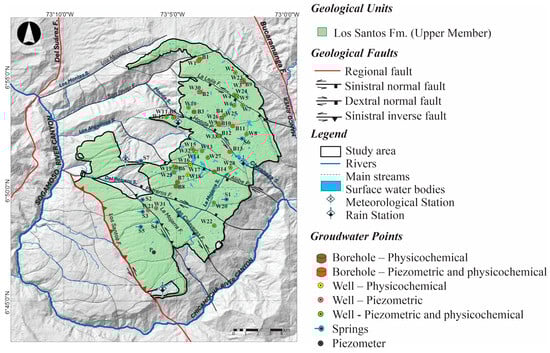
Figure 9.
Location of groundwater points inventoried in the study area.
Data on the average values of groundwater levels, electrical conductivity, pH, and temperature are presented in Table 2. The reported δ18O values represent averages in cases where periodic sampling showed no significant differences, indicating low temporal variability (less than 1‰ in δ18O). In contrast, minimum and maximum ranges are provided for cases with large temporal variability (greater than 1‰ in δ18O) or signs of evaporation.
Table 2.
Information on the inventoried water points in the study area.
Based on the piezometric level data from 35 points, three water levels could be identified using the k-means clustering algorithm in R-Studio, a statistical grouping method based on variance minimization (Figure 10). Based on this result, we hypothesize the presence of three distinct aquifers within the Upper Member, represented by clusters 1, 2, and 3. Considering the characteristics of each level, described below, we propose the following nomenclature to refer to the identified aquifers: Shallow Aquifer System (SAS), Upper Aquifer 1 (UA1), and Upper Aquifer 2 (UA2).
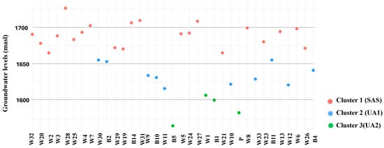
Figure 10.
Groundwater levels (m a.s.l.) in the three clusters.
4.2.1. Shallow Aquifer System (SAS)
The SAS is defined as a phreatic aquifer in depression areas with circulation in weathered and fractured levels of the Upper Member (cluster 1, Table 2, Figure 10), exhibiting water levels close to the surface, with average groundwater depths ranging from 0.5 to 11.2 m. The variation in topographic elevation among these points, ranging from 1665 to 1725 masl, prevents them from being connected under a regional flow system. If considered as such, the piezometric map would intersect the topography randomly, failing to reflect a coherent regional flow pattern.
Based on this, we propose an aquifer system with local flows in endorheic hydrographic zones, characterized by recharge areas ranging from 0.1 to 1 km2. This system includes: (i) mainly to the north, points associated with watersheds undergoing greater rainfall and therefore greater erosion, showing shallower water levels (0 to 2.2 m), where the vertical flow is limited due to the presence of an impermeable layer formed from by accumulations of clay generated by the hydrolysis of feldspar and the subsequent migration and deposition at the bottom, as well as by the erosion of fine grains deposited by the contributing catchment areas (ii) mainly to the south, points receiving less rainfall but where bodies of water are present, with deeper water levels (2.9 to 11.2 m), and water circulation occurring through weathered levels (thicknesses of 2.6 to 3.5 m) and fractured sandstone rocks, and limited by a local muddy strata found within the first 10 m of depth, as observed in columns C6 and C8. The southern region is not subjected to the same erosion process as in the northern part due to different climate regimes.
In the SAS, points are either associated with surface water bodies or areas with black soil development, or no specific association was identified. All points located in black soil development areas are found in the northern part of the study area (W2, W3, W4, W5, W7, W23, W24, W26) (Figure 9 and Table 2). This region is bounded to the south by the Honda Fault and is characterized by significant vegetation growth (Figure 2 and Figure 3).
The points associated with surface water bodies may or may not be related to black soil development. The interaction between surface water bodies and groundwater levels is determined through field observations and Oxygen-18 isotopic signature analyses. In the area, a local meteoric water line has been defined as δ2H = 8.22 × δ18O + 13.9, with rain-weighted annual average δ18O values of −8.51‰ in the north and −8.99‰ in the south [52]. The spatial pattern of more depleted precipitation values toward the south coincides with the spatial distribution of oxygen-18 in groundwater points with low temporal variability [52].
Points influenced by recharge from surface water bodies exhibit signs of evaporation in their isotopic composition, with enriched values of −3.05, −3.25, −3.74, and −5.12 ‰ δ18O and negative excess deuterium values of −6.7, −4.9, −5.5, −2.0‰ at points W8, W20, W28, and B14, respectively. In contrast, points where groundwater discharges into surface water bodies (i.e., where groundwater table elevations are higher than those of surface water bodies) do not show signs of evaporation.
Additionally, points exhibiting large temporal variability in isotopic behavior (W2, W4, W7, W19, W21) with δ18O values ranging from −9.04 to −1.07‰, are associated with rapid flows at short time steps (event or monthly scale) circulating through primary porosity enhanced by weathering processes and through fractures. Conversely, points with low temporal variability (W3, W5, W6, W13, W23, W24, W25, W27, W29), with δ18O values ranging from −6.59 to −8.3‰, suggest the presence of slower flows that promote water mixing, leading to a more stable isotopic signature. The difference between points showing large and low temporal isotopic variability may also be influenced by the size of the hydrographic basins where they are located. In small basins, each rainfall event represents a relatively large contribution compared to the total groundwater storage. Because the isotopic composition of precipitation can vary by more than 10‰ on a daily scale, individual rainfall events can strongly imprint their own isotopic signature on the aquifer, producing marked isotopic shifts throughout the year. In contrast, larger basins have greater storage and longer residence times, which favor mixing and attenuate short-term isotopic fluctuations, resulting in more stable groundwater signatures.
The physicochemical parameters of SAS indicate that low pH values (5.49 to 6.41) are found in points with black soil development (W2, W3, W4, W5, W7, W23, W24). Acidity is primarily related to the high organic matter content in the soil, which, in the presence of CO2, promotes organic matter oxidation and the release of carbonic acid. Meanwhile, average electrical conductivity ranges from low (24 to 101 μS/cm) to medium (111 to 277 μS/cm), with two points showing signs of contamination, W7 (EC: 634 μS/cm) and W25 (EC:736 μS/cm) characterized with high values of nitrates (>32 mg/L). The low-to-medium conductivity values are associated with groundwater-surface water interaction and the low mineralization capacity of silicates present in the weathered sandstones of the Upper Member.
4.2.2. Upper Aquifer 1 (UA1)
UA1 is represented by the points in cluster 2 (Table 2, Figure 10), where groundwater levels exhibit depth variations ranging from 0.7 to 37 m. The water table of each point was analyzed in relation to its neighbors, identifying hydraulic gradients between 0.001 and 0.01. This indicates a regional flow, shaping the first continuous aquifer within the Upper Member.
Based on the water table elevations (1607 to 1654.7 masl) and the topographic altitude it is proposed that UA1 is bordered by the muddy layer at the base of Segment D (see Section 4.1. Geological Model). A more detailed analysis will be provided in the Section 4.4. Conceptual Hydrogeological Model and Hypothesis on Water Resource Volumes, which integrate precise topographic data along with layer thicknesses and water table levels.
From the water table data, the piezometric map of UA1 was generated (Figure 11). The piezometric map reveals spatial variations in confidence associated with data density. The central portion of the study area, where most measurement points are located, exhibits the highest reliability in the interpolated hydraulic head distribution. In this central sector, the contours indicate a predominant E-W groundwater flow, consistent with both the regional dip of the sandstone layers and is enhanced by the fracture pattern and the SHmax (111°) identified by García-Arias et al. [45], which generates open fractures parallel to the E-W. In contrast, the northern and southern sectors show higher uncertainty due to the limited number of control points and the need for extrapolation. Nevertheless, the general trends remain hydrogeologically plausible. In the north, the piezometric gradients suggest a potential SE-NW flow aligned with the local topographic slope. In the south, the presence of several springs supports the interpretation of a NE-SW flow component, reflecting groundwater discharge in a direction consistent with the regional topographic gradient. Despite the increased uncertainty in these peripheral areas, the overall configuration of the piezometric surface provides a coherent representation of the aquifer’s flow system.
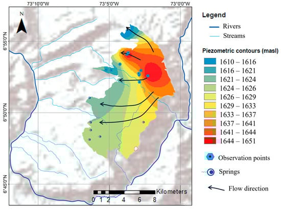
Figure 11.
UA1 piezometric map.
Based on the presented evidence, the existence of a fractured aquifer is proposed, consistent with the findings of Pinto et al. [47] and Díaz et al. [34], where fractures play a predominant role in groundwater flow circulation. Additionally, isotopic data mostly exhibit low temporal variability, with values of δ18O ranging between the points from −7.80 to −6.15 ‰, suggesting a significant rock storage capacity and efficient water mixing.
The recharge zone of UA1 is proposed to correspond to areas where the shallow aquifer system (SAS) is absent. It is important to note that the SAS is restricted to endorheic zones composed of weathered rock. Therefore, in areas where the rock remains unweathered, recharge to UA1 may occur. This hypothesis is supported by field observations, where topographic changes expose unweathered rock with visible fractures, suggesting that recharge may take place through these fractures. For future studies, it is recommended to carry out detailed mapping of weathered zones at scales finer than 1:5000 to better delineate the UA1 recharge areas. Additionally, the piezometric map shows that the highest water levels occur in the northern part of the study area, identifying a critical recharge zone that should be protected to prevent contamination.
Physicochemical parameters indicate slightly acidic pH values (5.41 to 6.36), similar to those observed in the SAS. This acidity may result from recharge processes in the northern zone, influenced by abundant vegetation and organic matter. Electrical conductivity ranges from low (21 to 102 μS/cm) to medium (208 to 325 μS/cm) values, interpreted similarly to those in the SAS, where the sandstone mineralogy contributes to water mineralization. Additionally, point B2 shows signs of anthropogenic contamination, with an EC of 325 μS/cm and 53.6 mg/L of nitrate.
4.2.3. Upper Aquifer 2 (UA2)
UA2 (segment C) is represented by the points in cluster 3 (Table 2, Figure 10). It is defined as a confined or semi-confined and fractured aquifer. Based on the geological model, where the presence of the upper part (segment D) is not observed in all columns, this aquifer may be at least partly or locally disconnected from UA1. However, the number of points with data from cluster 3 is too limited to identify the disconnected areas from the connected ones, and to construct accurate piezometric maps that would depict the direction of the water flow within this layer. In this work, the hypothesis of a disconnected aquifer is assumed, based on notably lower water table elevations than UA1 (1564 to 1600 m above sea level). This hypothesis implies that groundwater flows to deeper rock strata within the Upper Member in Segment C. This aquifer is bound by the impermeable Middle Member of the Los Santos Formation (segment B).
It is hypothesized that UA2 recharge processes may occur through water infiltration via deep faults and fractures. The relationship between UA1 and UA2 is further analyzed in Section 4.4. Isotopic data indicates both fast flows (high temporal variability) and slower flows (low temporal variability). However, due to the limited data available, isotopic and physicochemical analyses remain inconclusive.
4.3. Hydraulic Parameters
The analysis of the hydraulic parameters for each aquifer is based on field data (a pumping test conducted at point W32) and drilling reports. The data from the drilling reports is presented in Table 3 according to the range of groundwater levels representing UA1 and UA2. Table 3 presents the transmissivity and hydraulic conductivity values for three points representative of each aquifer. The data show that UA1 has a medium transmissivity (23.9 m2/day), while SAS and UA2 exhibit lower transmissivity values (3 m2/day and 2.4 m2/day, respectively).
Table 3.
Estimated hydraulic parameters of each aquifer.
Differences in transmissivity and hydraulic conductivity imply differences in groundwater flow mechanisms. UA1, classified as a fractured aquifer, has the highest groundwater velocity, associated with flow through fractures. In contrast, SAS and UA2 display slower flow rates, likely due to matrix-dominated circulation in UA2 and the presence of clay in the weathered rock matrix of SAS.
4.4. Conceptual Hydrogeological Model and Hypothesis on Water Resource Volumes
Based on the information obtained for the three aquifers identified in the Upper Member and integrating geological and topographic data, the following conceptual model of the groundwater system is proposed.
In endorheic areas, SAS levels are underlain by two types of mudstones: local depositional mudstones within the first 10 m of the Upper Member, which act as discontinuous delimiters of the aquifer, and pedogenic mudstones, formed through weathering (feldspar hydrolysis) and downward mobilization of fine sediments from the surface and slopes. These processes contribute to the formation of shallow and disconnected groundwater bodies. The SAS is also associated with wetland areas, with the northern zone characterized by abundant vegetation and organic-rich soils. The interaction between groundwater and wetlands may occur in both directions, with points where groundwater contributes to wetland flow and others where groundwater receives input from wetlands, regardless of the season.
UA1 is a phreatic and mainly fractured aquifer with water circulating within the rocks of segment D, as defined by Laverde [42], and contained by a basal mudstone layer. This level is present throughout most of the study area. However, towards the western and southern zones, it intersects the topography, leading to groundwater discharge, consistent with the regional flow direction (Figure 12). This is supported by the presence of springs in the southern sector and waterfalls along the western escarpments of the study area, such as Salto del Duende and Santa Rita.
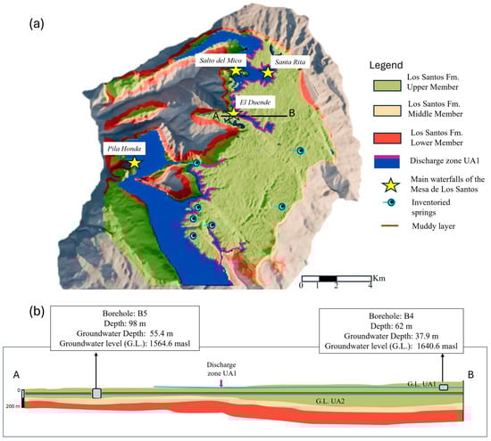
Figure 12.
(a) Model of the UA1 discharge zone. (b) Cross-section indicating the separation of UA1 and UA2 groundwater levels.
UA2 is a confined or semi-confined and fractured aquifer, where the groundwater flows through the sandstone layers at the base of the Upper Member of the Los Santos Formation, corresponding to segment C as proposed by Laverde [42]. It is assumed that the aquifer extends laterally throughout the Upper Member, presenting in some areas a connection with UA1 due to facies changes within the unit. It is proposed, as for UA1, that the flow direction follows the dip of the layers and the main fracture patterns oriented east–west, where the system discharge is also observed in waterfalls such as El Salto del Mico and Pila Honda (Figure 12).
Finally, integrating UA1 and UA2 groundwater level data with the 3D geological model highlights a separation between the two aquifers (Figure 12).
Using the 3D model, it was possible to estimate the storage capacity for UA1, considering the mean thickness of UA1’s saturated zone (25.5 m), the mean water table depth of 9.4 m, and the estimated area for UA1 of 103 km2 (area calculated considering the discharge zones). By applying a specific yield of sandstone ranging from 5% to 25% as reported in the literature [e.g., 58], the groundwater storage capacity of UA1 is estimated to range from 0.13 km3 to 0.65 km3.
In the case of UA2, due to limited data, information from well B5 was taken to estimate its groundwater reserves. Based on the average thickness of segments C (50 m) and D (46 m), and the depth to water level of 55.4 m, the saturated zone thickness is estimated at 40.6 m. Considering a surface area of 158 km2 (including the entire outcrop area of the Upper Member), and a specific yield ranging from 5% to 25%, the groundwater reserve is estimated to range between 0.32 km3 and 1.6 km3.
The estimated mean potential recharge for the study area is 133.8 mm/year. Converting this value into volume, based on the direct recharge area of each aquifer (103 km2 for UA1, which includes the SAS areas that are difficult to estimate but represent a negligible total area, and 55 km2 for the outcropping UA2 area), yields a recharge volume of 0.014 km3/year for UA1 and 0.007 km3/year for UA2. The direct recharge volume for UA1 results in a renewability period ranging between 9 and 46 years. In contrast, the direct recharge volume calculated for UA2 does not account for the water that may transfer from UA1 to UA2 as hidden recharge through vertical fractures, a process that may represent an important contribution. A rough estimate of the UA2 renewal rate may be determined by taking two extreme scenarios: (i) zero recharge from UA1 to UA2, where the direct recharge amounts to the volume of 0.007 km3/year, resulting in a renewability period between 46 and 228 years; (ii) 100% of the recharge of UA1 is discharged into UA2. In accordance with the principle of mass conservation, the recharge from UA1 to UA2 is assumed to be equivalent to the recharge of UA1 from precipitation, yielding a total recharge volume of 0.021 km3/year and a renewability period ranging between 16 and 80 years.
5. Conclusions
A 3D geological model of the Mesa de Los Santos was successfully developed integrating stratigraphic, lithological, and hydrological data. The model clearly represents the Lower, Middle, and Upper Members of the Los Santos Formation, providing a detailed spatial framework for hydrogeological analysis. Los Santos Formation hosts at least two major aquifer systems: the Lower Aquifer and the Upper Aquifer. The Lower Aquifer, formed by conglomeratic sandstone of the Lower Member, exhibits high primary porosity and secondary porosity associated with fractures, providing good hydrogeological potential. This aquifer is mostly confined by the impermeable Middle Member.
For the first time, three distinct aquifers were identified in the Upper Member of Los Santos Formation: Shallow Aquifer System (SAS), Upper Aquifer 1 (UA1) and Upper Aquifer 2 (UA2). This finding represents the main novel contribution of the study, highlighting the heterogeneity of the aquifer system and the importance of differentiating between local, phreatic, and confined or semi-confined groundwater flows. The SAS includes a number of groundwater bodies disconnected from each other. It is associated with topographic depressions and water table levels very close to the surface. In the northern zone, where there is greater rainfall and greater erosion, flows are maintained by impermeable layers formed by fine-grained sediments deposited by the contributing catchment areas. In this area, the SAS is associated with wetlands, with greater vegetation abundance and the development of black soil. In the southern zone, SAS flows circulate through levels of weathered and fractured sandstone and are supported by clayey levels within the first 10 m of depth in the Upper Member. In the SAS, a relationship with surface water bodies is observed, with isotopic signatures showing signs of evaporation prior to infiltration.
UA1 is a phreatic and fractured aquifer that flows through segment D of the Upper Member and is contained by the muddy level demarcating segments C and D, with an E-W flow consistent with the dip of the layers and the main directions of the fracture patterns and an important recharge zone to the north of the study area. The isotopic data mostly exhibits low temporal variability suggesting a significant rock storage capacity and efficient water mixing. A renewability period ranging between 9 and 46 years has been estimated for this aquifer.
UA2 is a confined or semi-confined and fractured aquifer that flows through segment C of the Upper Member and is underlain by the impermeable Middle Member. The main recharge process may occur through water infiltration via deep faults and fractures. Isotopic data indicates both fast flows (high temporal variability) through fractures, and slower flows (low temporal variability), which are more efficiently mixed in storage. However, due to the limited data available, isotopic and physicochemical analyses remain inconclusive as to its detailed hydrologic behavior. A renewability period ranging between 16 and 228 years has been estimated for this aquifer.
This study provides important insights for hydrogeology in general. The integration of UAV-derived data allowed a detailed characterization of the Upper Member stratigraphy, improving the spatial resolution and accuracy of the geological model. Furthermore, the study highlights the complexities in groundwater flow induced by fracture patterns, topographic position, and localized internal drainage, as well as flows through weathered rock, which influence the connectivity and recharge of the three identified aquifers. These findings demonstrate the value of combining high-resolution topographic data with hydrogeological and isotopic information to understand heterogeneous aquifer systems, providing a framework that can be applied to similar hydrogeological settings elsewhere.
Finally, the characterization of UA2 and the SAS was constrained by limited piezometric and isotopic data. Future studies should expand spatial coverage, include additional isotopic and physicochemical analyses, and refine numerical models to better quantify flow and storage in all aquifers.
Author Contributions
Conceptualization, M.C., S.G., J.-D.T. and F.V.; methodology, M.C.; software, A.S., E.D., M.C.-H. and J.S.; validation, J.-D.T., S.G., F.V. and N.P.; formal analysis, M.C.; investigation, M.C., A.S., E.D., M.C.-H. and J.S.; resources, F.V.; data curation, M.C., A.S., E.D., M.C.-H. and J.S.; writing—original draft preparation, M.C.; writing—review and editing, M.C., S.G., F.V., J.-D.T. and N.P.; visualization, M.C., E.D. and M.C.-H.; supervision, J.-D.T.; project administration, F.V.; funding acquisition, F.V. All authors have read and agreed to the published version of the manuscript.
Funding
This research was funded by Universidad Industrial de Santander, through the project “Estudio Integral del Agua en la Mesa de los Santos” (code 2534).
Data Availability Statement
The authors declare that the data supporting the findings of this study are available within the paper.
Acknowledgments
The authors thank the community of Mesa de Los Santos for allowing access to the inventoried water points.
Conflicts of Interest
The authors declare no conflicts of interest.
Abbreviations
The following abbreviations are used in this manuscript:
| SAS | Shallow Aquifer System |
| UA1 | Upper Aquifer 1 |
| UA2 | Upper Aquifer 2 |
| EC | Electrical Conductivity |
| pH | Potential of hydrogen |
| T | Temperature |
| SWB | Soil water balance |
| IDEAM | Instituto de Hidrología, Meteorología y Estudios Ambientales |
| GPH | Research Group on Water Resources and environmental sanitation |
| UAV | Unmanned Aerial Vehicles |
| DOM | Digital Outcrop Models |
| DEM | Digital Elevation Model |
| C | Column |
| masl | Meters above sea level |
| SHmax | Maximum horizontal tensor |
References
- Conti, K.I.; IGRAC; University of Amsterdam. Groundwater in the Sustainable Development Goals; IGRAC: The Hague Area, The Netherlands, 2015. [Google Scholar]
- United Nations. Sustainable Development Goal 6 Synthesis Report 2018 on Water and Sanitation; United Nations: New York, NY, USA, 2018. [Google Scholar]
- UNESCO. The United National World Water Development Report 2022. Groundwater: Making the Invisible Visible. 2022. Available online: https://unesdoc.unesco.org/ark:/48223/pf0000380721 (accessed on 1 March 2024).
- Bridge, J.S.; Hyndman, D.W. (Eds.) Aquifer Characterization; Special Publication No. 80; SEPM: Tulsa, OK, USA, 2004. [Google Scholar]
- Allen, P.A.; Allen, J.R. Basin Analysis: Principles and Application to Petroleum Play Assessment; John Wiley & Sons, Ltd.: Hoboken, NJ, USA, 2013. [Google Scholar]
- Yuan, G.; Cao, Y.; Schulz, H.M.; Hao, F.; Gluyas, J.; Liu, K.; Li, F. A review of feldspar alteration and its geological significance in sedimentary basins: From shallow aquifers to deep hydrocarbon reservoirs. Earth-Sci. Rev. 2019, 191, 114–140. [Google Scholar] [CrossRef]
- Cendón, D.I.; Hankin, S.I.; Williams, J.P.; Van der Ley, M.; Peterson, M.; Hughes, C.E.; Chisari, R. Groundwater residence time in a dissected and weathered sandstone plateau: Kulnura–Mangrove Mountain aquifer, NSW, Australia. Aust. J. Earth Sci. 2014, 61, 475–499. [Google Scholar] [CrossRef]
- Worthington, S.R.; Davies, G.J.; Alexander, E.C., Jr. Enhancement of bedrock permeability by weathering. Earth-Sci. Rev. 2016, 160, 188–202. [Google Scholar] [CrossRef]
- Bertassello, L.E.; Rao, P.S.C.; Jawitz, J.W.; Aubeneau, A.F.; Botter, G. Wetlandscape hydrologic dynamics driven by shallow groundwater and landscape topography. Hydrol. Process. 2020, 34, 1460–1474. [Google Scholar] [CrossRef]
- Van der Kamp, G.; Hayashi, M. Groundwater-wetland ecosystem interaction in the semiarid glaciated plains of North America. Hydrogeol. J. 2009, 17, 203. [Google Scholar] [CrossRef]
- Carol, E.; Pilar Alvarez, M.D.; Santucci, L.; Candanedo, I.; Arcia, M. Origin and dynamics of surface water-groundwater flows that sustain the Matusagaratí Wetland, Panamá. Aquat. Sci. 2022, 84, 16. [Google Scholar] [CrossRef]
- Medjani, F.; Djidel, M.; Labar, S.; Bouchagoura, L.; Rezzag Bara, C. Groundwater physico-chemical properties and water quality changes in shallow aquifers in arid saline wetlands, Ouargla, Algeria. Appl. Water Sci. 2021, 11, 82. [Google Scholar] [CrossRef]
- Jourde, H.; Cornaton, F.; Pistre, S.; Bidaux, P. Flow behavior in a dual fracture network. J. Hydrol. 2002, 266, 99–119. [Google Scholar] [CrossRef]
- Bense, V.F.; Gleeson, T.; Loveless, S.E.; Bour, O.; Scibek, J. Fault zone hydrogeology. Earth-Sci. Rev. 2013, 127, 171–192. [Google Scholar] [CrossRef]
- Medici, G.; West, L.J.; Mountney, N.P. Characterizing flow pathways in a sandstone aquifer: Tectonic vs sedimentary heterogeneities. J. Contam. Hydrol. 2016, 194, 36–58. [Google Scholar] [CrossRef]
- Batlle-Aguilar, J.; Banks, E.W.; Batelaan, O.; Kipfer, R.; Brennwald, M.S.; Cook, P.G. Groundwater residence time and aquifer recharge in multilayered, semi-confined and faulted aquifer systems using environmental tracers. J. Hydrol. 2017, 546, 150–165. [Google Scholar] [CrossRef]
- Tóth, E.; Hrabovszki, E.; Schubert, F.; Tóth, T.M. Lithology-controlled hydrodynamic behaviour of a fractured sandstone–claystone body in a Radioactive Waste Repository Site, SW Hungary. Appl. Sci. 2022, 12, 2528. [Google Scholar] [CrossRef]
- Huang, Q.; Angelier, J. Inversion of field data in fault tectonics to obtain the regional stress-II using conjugate sets within heterogeneous families for computing palaeostress axes. J. Geophys. 1989, 96, 139–149. [Google Scholar] [CrossRef]
- Fossen, H. Structural Geology; Cambridge University Press: Cambridge, UK, 2010; p. 463. [Google Scholar]
- Davis, G.; Reynolds, S.; Kluth, C. Structural Geology of Rocks and Regions, 3rd ed.; John Wiley & Sons: New York, NY, USA, 2012; p. 861. [Google Scholar]
- Worthington, S.R. Diagnostic tests for conceptualizing transport in bedrock aquifers. J. Hydrol. 2015, 529, 365–372. [Google Scholar] [CrossRef]
- FUNDEMESA. Mesa de los Santos. In Memorias del Paraíso; Fundación para el Desarrollo de la Mesa de los Santos: Bucaramanga, Colombia, 2009; p. 96. [Google Scholar]
- Prieto-Jiménez, D.; Oviedo-Ocaña, E.R.; Gómez-Isidro, S.; Domínguez, I.C. A multicriteria decision analysis for selecting rainwater harvesting systems in rural areas: A tool for developing countries. Environ. Sci. Pollut. Res. 2024, 31, 42476–42491. [Google Scholar] [CrossRef]
- Bredehoeft, J. The conceptualization model problem—Surprise. Hydrogeol. J. 2005, 13, 37–46. [Google Scholar] [CrossRef]
- Anderson, M.P.; Woessner, W.W.; Hunt, R.J. Modeling Purpose and Conceptual Model. In Applied Groundwater Modeling; Anderson, M.P., Woessner, W.W., Hunt, R.J., Eds.; Elsevier Inc.: San Diego, CA, USA, 2015; pp. 27–67. [Google Scholar]
- Enemark, T.; Peeters, L.J.; Mallants, D.; Batelaan, O. Hydrogeological conceptual model building and testing: A review. J. Hydrol 2019, 569, 310–329. [Google Scholar] [CrossRef]
- Blavoux, B.; Letolle, R. Apports des techniques isotopiques á la connaissance des eaux souterraines (Contribution of isotopic tools to the knowledge of groundwaters). Geochronique 1995, 54, 12–15. [Google Scholar]
- Gonfiantini, R.; Roche, M.A.; Olivry, J.C.; Fontes, J.C.; Zuppi, G.M. The altitude effect on the isotopic composition of tropical rains. Chem. Geol. 2001, 181, 147–167. [Google Scholar] [CrossRef]
- Cetina, M.; Taupin, J.D.; Gómez, S.; Patris, N. Hydrodynamic conceptual model of groundwater in the headwater of the Rio de 774 Oro, Santander (Colombia) by geochemical and isotope tools. Water Supply 2020, 20, 1567–1579. [Google Scholar] [CrossRef]
- Hamidi, M.D.; Gröcke, D.R.; Joshi, S.K.; Greenwell, H.C. Investigating groundwater recharge using hydrogen and oxygen stable isotopes in Kabul city, a semi-arid region. J. Hydrol. 2023, 626, 130187. [Google Scholar] [CrossRef]
- Wang, L.; Sun, Y.; Yang, C.; Dong, Y. Groundwater–surface water interactions across an arid river basin: Spatial patterns revealed by stable isotopes and hydrochemistry. Hydrol. Earth Syst. Sci. 2025, 29, 4417–4436. [Google Scholar] [CrossRef]
- CNPV. Censo Nacional de Población y Vivienda. 2018. Available online: https://www.dane.gov.co/index.php/estadisticas-por-tema/demografia-y-poblacion/censo-nacional-de-poblacion-y-vivenda-2018 (accessed on 17 March 2021).
- CNA. Censo Nacional Agropecuario. 2014. Available online: https://www.datos.gov.co/widgets/6pmq-2i7c (accessed on 17 March 2021).
- Díaz, E.J.; Contreras, N.M.; Pinto, J.E.; Velandia, F.; Morales, C.J.; Hincapie, G. Evaluación hidrogeológica preliminar de las unidades geológicas de la Mesa de los Santos, Santander. Bol. Geol. 2009, 31, 61–70. [Google Scholar]
- Moreno, M.L.; Silva, K.D. Identificación de Ambientes Geomorfológicos y Elaboración de un Mapa de Favorabilidad para la Percolación de la Zona de la Mesa de Los Santos, Santander. In Trabajo de Grado Para Optar Por el Título de Geólogo; Universidad Industrial de Santander: Bucaramanga, Colombia, 2021. Available online: https://noesis.uis.edu.co/handle/20.500.14071/41138 (accessed on 1 February 2025).
- Becerra, N.J.; Parra, C.G. Balance Hídrico para Estimar Recarga Potential en la Mesa de Los Santos y Dirección de Flujo de Aguas Subterráneas. In Trabajo de Grado Para Optar Por el Título de Ingeniero Civil; Universidad Industrial de Santander: Bucaramanga, Colombia, 2016. Available online: https://noesis.uis.edu.co/handle/20.500.14071/33946 (accessed on 1 February 2025).
- Garzón, Y.X.; Salcedo, H.D. Estimación de la Recarga Potencial Mensual en La Mesa de Los Santos (Santander). In Trabajo de Grado Para Optar Por el Título de Ingeniero Civil; Universidad Industrial de Santander: Bucaramanga, Colombia, 2022. Available online: https://noesis.uis.edu.co/handle/20.500.14071/9902 (accessed on 1 February 2025).
- Julivert, M. La morfoestructura de la zona de Mesas al SW de Bucaramanga (Colombia, S.A). Bol. Geol. 1958, 1, 7–43. [Google Scholar]
- Julivert, M.; Barrero, D.; Navas, J. Geología de la Mesa de Los Santos. Bol. Geol. 1964, 18, 5–11. [Google Scholar]
- Ward, D.; Goldsmith, R.; Cruz, J.; Jaramillo, L.; Vargas, R. Geología del Cuadrángulo Pamplona H-12, escala 1:100.000; Instituto Colombiano de Geología Y Minas: Bogotá, Colombia, 1977.
- Julivert, M.; Tellez, N. Sobre la presencia de fallas de edad pre-Cretácica y post-Girón (Jura-Triásico) en el flanco W del Macizo de Santander (Cordillera Oriental de Colombia). Bol. Geol. 1963, 12, 5–17. [Google Scholar]
- Laverde, F. La Formación Los Santos: Un depósito continental anterior al ingreso marino del Cretácico. In Proyecto Cretácico; Etayo-Serna, F., Laverde, F., Eds.; Contribuciones: Ingeominas Publicaciones Geológicas Especiales 16; Instituto Nacional de Investigaciones Geológico-Mineras (INGEOMINAS): Bogotá, Colombia, 1985; pp. xx-1–xx-24. [Google Scholar]
- Laverde, F. Revisiting the latest Jurassic-earliest Cretaceous Los Santos Formation, Eastern Cordillera of Colombia. A–The history of its origin and the lowermost part of the unit. Boletín Geológico 2023, 50, 689. [Google Scholar] [CrossRef]
- Laverde, F.L. Revisiting the latest Jurassic-earliest Cretaceous Los Santos Formation, Eastern Cordillera of Colombia. B–A transgressive river mouth deposit in a syntectonic scenario. Boletín Geológico 2023, 50, 690. [Google Scholar] [CrossRef]
- García-Arias, S.; Velandia, F.; Alvarez, A.; Sanabria-Gómez, J.D.; Tarazona, Y.; Vargas, M.C. Stress tensors and quantification of fracture patterns to analyze connectivity and potential fluid flow in a mesa landform of the Northern Andes. J. Mt. Sci. 2024, 21, 271–291. [Google Scholar] [CrossRef]
- Langenheim, R.L. Preliminary report on the stratigraphy of the Giron Formation in Santander and Boyacá. Bol. Geol. 1959, 3, 35–40. [Google Scholar]
- Pinto, J.E.; Clavijo, J.; Gómez, S.; Bermoudes, O. Geological and hydrogeological research project in Mesa de Los Santos, northeast sector of Curití and western edge of the Santander Massif, department of Santander. In Explanatory Report on the Geological and Hydrogeological Research in Mesa de Los Santos and the Northeast Sector of Curití; Instituto Colombiano de Geología y Minería: Bucaramanga, Colombia, 2007. [Google Scholar]
- Ingeominas. Informe Hidrogeológico de la Mesa de Los Santos; Instituto de Investigaciones e Información Geocientífica Minero-Ambiental y Nuclear (Ingeominas, ahora Servicio Geológico Colombiano): Bogotá, Colombia, 2009; p. 75.
- Velandia, F.; Bermúdez, M.A. The transpressive southern termination of the Bucaramanga fault (Colombia): Insights from geological mapping, stress tensors, and fractal analysis. J. Struct. Geol. 2018, 115, 190–207. [Google Scholar] [CrossRef]
- Diederix, H.; Bohórquez, O.P.; Mora–Páez, H.; Peláez, J.R.; Cardona, L.; Corchuelo, Y.; Ramírez, J.; Díaz–Mila, F. Quaternary activity of the Bucaramanga Fault in the Departments of Santander and Cesar. In The Geology of Colombia, Quaternary; Gómez, J., Pinilla–Pachon, A.O., Eds.; Publicaciones Geológicas Especiales 38; Servicio Geológico Colombiano: Bogotá, Colombia, 2020; Volume 4, pp. 453–477. [Google Scholar] [CrossRef]
- Casadiegos-Agudelo, L.; Cetina-Tarazona, M.A.; Dominguez-Rivera, I.C.; Gomez-Isidro, S. Validation of the intrinsic vulnerability to pollution of fractured siliciclastic aquifers using natural background levels. Groundw. Sustain. Dev. 2024, 25, 101143. [Google Scholar] [CrossRef]
- Cetina, M.A.; Taupin, J.D.; Gómez, S.; Patris, N. Isotope study of monthly rainfall and its response in the Santos Formation phreatic aquifer, Mesa de Los Santos, Santander (Colombia). Proc. IAHS 2024, 385, 231–237. [Google Scholar] [CrossRef]
- Sarmiento-Rojas, L.; Van Wess, J.; Cloetingh, S. Mesozoic transtensional basin history of the eastern Cordillera, Colombian Andes: Inferences from tectonic models. J. S. Am. Earth Sci. 2006, 21, 383–411. [Google Scholar] [CrossRef]
- Araque Gómez, C.N.; Otero-Ramírez, J.L. Zonas Transversales y su Relación con Estructuras Regionales, Flanco O-Cordillera Oriental. In Trabajo de Grado Para Optar Por el Título de Geólogo; Universidad Industrial de Santander: Bucaramanga, Colombia, 2016. Available online: https://noesis.uis.edu.co/handle/20.500.14071/35014 (accessed on 1 February 2025).
- Singhal, B.B.S.; Gupta, R.P. Applied Hydrogeology of Fractured Rocks; Springer Science & Business Media: Dordrecht, The Netherland, 2010. [Google Scholar]
Disclaimer/Publisher’s Note: The statements, opinions and data contained in all publications are solely those of the individual author(s) and contributor(s) and not of MDPI and/or the editor(s). MDPI and/or the editor(s) disclaim responsibility for any injury to people or property resulting from any ideas, methods, instructions or products referred to in the content. |
© 2025 by the authors. Licensee MDPI, Basel, Switzerland. This article is an open access article distributed under the terms and conditions of the Creative Commons Attribution (CC BY) license (https://creativecommons.org/licenses/by/4.0/).