Abstract
In December 2013, a portion of a large and deep ancient landslide on the southern slope of the Montescaglioso town (Basilicata, Southern Italy) was abruptly reactivated, as a consequence of exceptional rainfall events, causing relevant damages to structures and infrastructures. The sliding surface is supposed to be located within a thick deposit of Pleistocene stiff clays overlain by dislocated blocks of calcarenites and cemented conglomerates. This paper discusses the research carried out to investigate the failure mechanism that occurred during the landslide event and the factors that controlled the reactivation. To this purpose, geological and geomorphological analyses were first proposed, followed by a back-analysis of the landslide process, performed via limit equilibrium calculations implementing time-dependent pore water pressure distributions derived from transient seepage finite element analyses. Furthermore, the overall landslide mechanism was investigated through a three-dimensional finite element analysis, built using the monitoring campaign carried out in the post-failure stage and calibrated according to the in situ failure mechanism evidence. Both the limit equilibrium and finite element analyses provide results in good agreement with the geomorphological evidence, further allowing us to recognize the effects of rainfall infiltration in the increase of pore water pressure along the sliding surface and the variation of the stress–strain state leading to failure occurrence.
1. Introduction
The occasional reactivation of earth-slides in clay formations along pre-existing shear bands, where critical state or residual strength is operative, can be characterized, in some cases, by high displacement rates [1], and this still represents a challenging topic for hazard assessment. The occasional renewal of earth-slide movements along pre-existing shear bands at residual strength generally takes place with slow and relatively limited displacements, due to the essentially non-brittle behavior of the slip surface [1,2,3]. However, under some circumstances, abrupt and rapid occasional reactivations of earth-slides, with large and rapid mass displacements, may occur over a very short period as a consequence of a specific trigger. Several mechanisms potentially leading to large and rapid earth-slide reactivations have been proposed [1,4], which include the following: rapid pore-pressure increase at the slip surface, due to preferential seepage flows [5], water filling of tension cracks, or rear scarps in the upper landslide area; breaking of pipelines crossing the slide area; impedance of normal outflow of groundwater from the slope; stress changes due to manmade excavation or natural erosion at the toe; rapid change in load distribution along the shear surface; and internal brittleness within the landslide mass for compound and roto-translational slides. In particular, ref. [4] points out that considerable displacements may occur as a consequence of the development of new portions of the failure surface in the toe region on low-angle thrust shears or in those cases where the slide mass consists of soil or rock with brittle stress–strain behavior (litho-relicts in particular). In such a context, the whole failure mechanism, which involves the pre-existing sliding surface and the newly formed brittle failure at the toe, may still have a degree of brittleness, possibly leading to significant movements taking place in a relatively short time span. It follows that a high level of hazard may arise from landslide processes where the aforementioned factors play a role, bringing about severe damage to the interacting structures and potentially threatening human lives which can be reduced by using predictive and early warning tools [6,7,8]. On 3 December 2013, a large earth-slide occurred along the southern hillslope of the Montescaglioso town (Basilicata, Southern Italy), causing significant damage to some buildings and the interruption of relevant road infrastructure. The landslide activation took place after about 52 h of high-intensity rainfalls, representing an exceptional rainfall event for the specific area. The about 10 km2 landslide was characterized by large horizontal and vertical displacement components (maximum horizontal displacement at the toe approximately 20 m), which took place in a very short time (15 min). Due to the readiness of inhabitants living in the buildings and of car drivers passing through the landslide area at the time of failure, no injury or death was recorded. As described below in more detail, the slip surface is supposed to be located within a thick deposit of stiff overconsolidated clays, locally overlain by large blocks of calcarenites and cemented breccias, resulting from ancient landslide processes. According to the geomorphological evidence and the historical data, the landslide lies in a wider area affected in the past by large slope movements [9]. Thus, the examined phenomenon can be classified as an occasional reactivation along a portion of pre-existing shear surfaces [1,10]. This was also confirmed by mapping of the surface features produced by the landslide, carried out in the immediate days after the event [11]. Pellicani et al. [12,13] presented an application of multi-temporal LiDAR and UAV techniques to interpret the geomorphological and kinematical evolution of the December 2013 Montescaglioso landslide. They highlighted the features of a progressive failure, with a rigid translation in the lower part and subsequent retrogressive propagation. Several applications of SAR interferometry techniques have been also performed on the Montescaglioso landslide, due to the favorable conditions of the landslide geometry [14,15,16,17,18]. All of these works provide consistent results in terms of landslide kinematics. However, the aforementioned papers do not focus on the landslide mechanism or on the factors that have controlled the landslide reactivation.
The present paper proposes a back-analysis of the 2013 Montescaglioso landslide, aimed at assessing the main triggering and aggravating factors that were responsible for its high mobility. This is first pursued through a detailed analysis of the geomorphological features of the case study, followed by a geotechnical characterization of involved soils. Later on, a two-dimensional seepage finite element analysis is presented aimed at exploring the transient seepage process that followed water infiltration from the ground surface. Furthermore, a limit equilibrium analysis implementing the step-by-step pore water pressure distributions varying with time, as result of the transient seepage analysis, is discussed. The objective was to study the variation of the slope stability conditions during the whole rainfall event. Finally, a three-dimensional stress–strain finite element analysis investigated the overall failure mechanism in terms of the extent of the unstable area, soil failure evolution within the slope, and strength mobilized along the shear surface. The 3D model also allowed us to gain an insight into the overall landslide displacement field, e.g., landslide directivity and areal distribution of displacement components, which results in good agreement with the in situ landslide mobility, as reconstructed from geomorphological evidence, Digital Terrain Model surveys, and satellite remote-sensing analyses. Recently, three-dimensional finite element models have been increasingly used to investigate the stress–strain evolution of slopes, thus providing insights in the landslide behavior [19,20,21,22]. The study performed in this paper leads to advancements regarding the main factor considered responsible for the rapid reactivation of the landslide, i.e., the rapid pore-pressure increases due to rainfall infiltration within the slope, even along the slip surface. However, some other factors, such as the rupture of a large aqueduct pipeline crossing the slide area, the long-term stress changes due to river erosion at the toe, and the brittle activation of new portions of the failure surface at the scarp area and in the toe region (both connected with a low-angle pre-existing shear surface), could have played additional roles in the landslide reactivation, too.
2. The 2013 Montescaglioso Landslide
2.1. Features of the Landslide Reactivation
Between October 2013 and the beginning of December 2013, the area around the Montescaglioso town (Matera province, Southern Italy) (Figure 1) was hit by two severe rainfall events. The first (5–8 October, cumulative rainfall was 246 mm, and mean rainfall intensity was 3.6 mm/h) affected a large area between Apulia and Basilicata, causing several landslides and floods, four casualties, and huge economic damages. Two months later, another rainfall event (30 November–3 December, cumulative rainfall was 151.6 mm, and duration was 56 h), hit the same area and triggered a large earth-slide on December 3 along the southern hillslope of the town [11,14]. Taking into account the pluviometric regime of the area, characterized yearly by a value of 570 mm, this second event corresponds to 27% of the average annual rainfall and 81% of the maximum monthly rainfall.
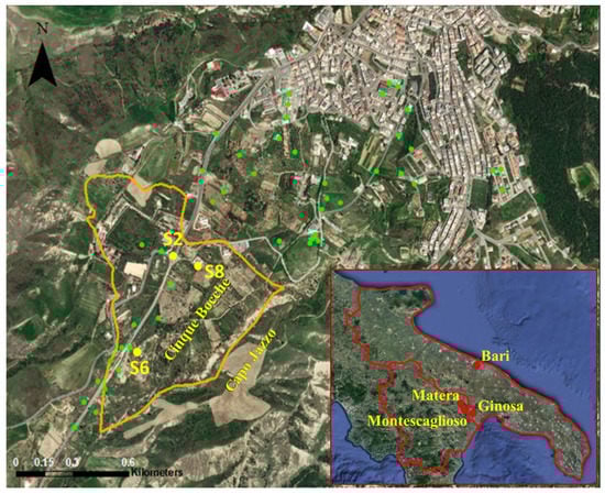
Figure 1.
Aerial view of the Montescaglioso area (location in the inset) and its SW hillslope, with the landslide area in orange and locations of the Cinque Bocche and Capo Jazzo streams. In green are the locations of the boreholes performed throughout the area during several campaigns, and in yellow are the locations of the boreholes drilled after the landslide event and equipped with inclinometers (S2, S6, S8).
The landslide initiation and evolution were reconstructed based on the information collected from direct witnesses: it started at ca. 13.00 CET on 3 December, quickly exhausting its most intense phase and immediately causing the destruction of a 500 m stretch of the freeway connecting Montescaglioso to Province Road SP175 (Figure 2).
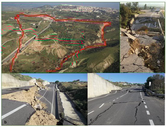
Figure 2.
Aerial view of the landslide area and some of the most relevant damage to the infrastructures in the affected area. Labels (a, b, c) indicate the location of the pictures in the aerial view.
Later on, the movement involved the lower-left flank of the landslide, resulting in the formation of a swarm of scarps and counterscarps (Figure 2), several tens of meters in length, and creating a series of trenches with a maximum depth of seven to eight meters [11,23]. The whole surface of the landslide area (about 5 × 10⁵ m2) directly affected some private houses and warehouses, which were subjected to rigid body translation for few meters downslope and tilting, while a grocery store located in the crown area collapsed (Figure 3). Luckily, no direct damage to people was recorded, despite the rapid activation of the landslide, since the evolution and the consequent deformation of the buildings were relatively slow, allowing the inhabitants to avoid fatal consequences.
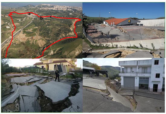
Figure 3.
Aerial view of the landslide area and the main effects on buildings. Labels (a, b, c) indicate the location of the pictures in the aerial view.
2.2. Geological and Geomorphological Features
The Montescaglioso village is located at the top of a hill, at about 350 m a.s.l., in the final reach of the Bradano river alluvial plain. The hill is bounded by steep slopes that are affected by the widespread development of landslides of different typologies, showing a variable state of [9,14,23], indicating that the area is highly prone to mass movements. The landslide area is located just below the urban area and the cemetery, between the Cinque Bocche and Fosso di Capo Jazzo streams (Figure 1).
The geological setting is characterized by sediments of the Bradanic Trough, which represents the foredeep where the Apulian foreland subsidies under the Southern Apennines [15]. The Lower–Middle Pleistocene sediments [17,24] are represented by a regressive sequence, locally covered along the slope interested by the 2013 landslide by fluvial conglomerates. In detail, Sub-Apennine Clays crop out in the area, delimited at the top by the Montemarano sands and the Irsina conglomerates [25,26,27,28,29,30]. The overall sequence of clays, sands, and conglomerate crops out at the upper hillslope, while the clays are interbedded by sandy/arenaceous layers in the middle lower portion [23]. Along the slope, where erosion processes are widespread, chaotic large blocks related to ancient gravitational phenomena are common [15]. The general structural setting of the area is characterized by tectonic lineaments with NW-SE and SW-NE orientations, which play a fundamental role in the development of the fluvial network at the regional scale. Based on borehole stratigraphies, a geological longitudinal section was reconstructed (Figure 4), and a fault system was recognized in the crown area.
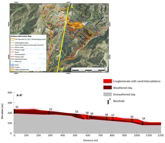
Figure 4.
Geological longitudinal cross-section of the landslide area. In the sketch, the geomorphological map (modified from [11]) and the section trace are shown.
As concerns the hydraulic conditions, two different types of groundwater circulation were found along the slope: a superficial regime affecting the debris shallow layer (between 2 and 6 m from the ground surface) and a deep groundwater regime affecting the lower clays [23].
Pre- and post-event orthophotos and LIDAR data were used by several authors to analyze the ground surface deformation associated with landslide reactivation [13,14,17,23]. The comparison between pre- and post-event Digital Terrain Models (DTMs) highlighted a strong horizontal N–S component in the landslide movement, along with a general lowering of the ground surface within its middle–upper portion, as well as an uplift of a few meters at the landslide toe.
The data derived from the inclinometer readings showed a remarkably low—about negligible—progression of the movement in the post-failure stage, as discussed in detail later on. In particular, very small shear displacements were measured at about 50 m depth in the toe area and at 10–20 m depth near the main landslide scarp. These inclinometer deformations were interpreted as representative of weakness zones and, as such, of the shear band.
3. Geotechnical Parameters of the Soils
The clays lying at depth in the examined slope belong to the Sub-Apennine Clays Formation [27], which has been deeply investigated in the geotechnical literature [31,32,33,34,35].
Amanti et al. [23] have presented the results of detailed geotechnical investigations carried out on clay samples taken from the landslide area during post-event field surveys. In particular, samples were collected both from block sampling in the shallowest layers of the crown area and from boreholes drilled to depths varying from 25 m to 66 m. Based on these laboratory tests, the physical and mechanical properties of involved soils are fairly homogeneous, with rather limited variability in depth. The grain size distribution of clay samples is fairly homogeneous, mainly consisting of silty and sandy clays, with clay fraction varying from 38 to 55%. The plasticity index ranges between 22 and 41%. These being typical values also for clays from different areas but belonging to the same formation [32,33,34]. Based on the Casagrande chart, the soils can be classified as characterized by medium to high plasticity and low activity. The average natural unit weight is 20 kN/m3, whereas the natural water content is about 20%. Based on the results of oedometer tests, the clays can be classified as overconsolidated, with OCR ranging between 1.7 and 7.4. Direct-shear tests have indicated cohesion values at peak ranging between 20 and 40 kPa, with friction angles in the range of 19–30°. Whereas consolidated/undrained triaxial tests have shown an average value of the peak cohesion equal to 30 kPa and a friction angle of 28°, the latter being higher than the values generally found for the same formation. Such a discrepancy is supposed to be related to the possible higher sand component of the samples used for the shear tests. The residual friction angle has been estimated through ring shear tests and results to be in a range lower than the minimum value of the aforementioned range of the peak friction angle [23].
For Sub-Apennine Clays outcropping at other sites, Cafaro and Cotecchia (2001) [32] and Lollino et al. (2005) [33] found a plasticity index in the range of 25–33%, a liquid limit between 50 and 60 %, and a permeability coefficient in the range from 3 to 6 × 10⁻¹¹ m/s. At other sites in the northern Apulian Foreland, [34] indicate plasticity index values in the range of 22–28%, void ratio in the range of 0.5–0.6, as well as a cohesion value equal to 30 kPa, and friction angle of 22°, based on consolidated/undrained triaxial tests. In this case, the permeability coefficient is found to be about 7 × 10⁻¹¹ m/s. Similar values were found by Di Maio and Vassallo [35] for Sub-Apennine Clays outcropping in a landslide area close to Montescaglioso.
Based on the large dataset available on the geotechnical characterization of the clay formation, and specifically on the deposits cropping out in the landslide area, the hydraulic and mechanical properties, summarized in Table 1, have been chosen as representative of the clay behavior. From a geotechnical point of view, the weathered clay and unweathered clay layers were unified into a single geo-lithotechnical layer, given the equality of physical and mechanical parameters.

Table 1.
Soil hydraulic and mechanical parameters adopted in the seepage FEM and LE analyses.
4. Hydrological Processes and Landslide Reactivation
A back-analysis of the December 2013 landslide reactivation was performed through the limit equilibrium method calculations implementing time-dependent pore water pressure distributions derived from transient-seepage finite-element analyses. The aim was to investigate the influence of rainfall infiltration and pore water pressure variations on the change in stability factor during the rainfall event. The limit equilibrium analyses were performed by using SLOPE/W [36], adopting the Morgenstern and Price (1965) method [37]. Transient finite element analyses were carried out with SEEP/W [36] to define the time-varying pore water pressure distributions resulting from the rainfall infiltration process within the slope to implement in the LEM analyses.
The stratigraphic scheme adopted for the calculation was assumed according to the geological longitudinal section shown in Figure 4. Figure 5 shows the finite element mesh adopted for the seepage analysis. The geometry of the sliding surface was assumed to be in accordance with in situ geomorphological evidence [11], as well as with borehole and inclinometer data. In particular, the assumed sliding surface delimits a roto-translational landslide body, with the scarp approximately at an elevation of 200 m a.s.l. and the depth of the failure surface increasing downslope (between 10 and 20 m from g.l. in the upper part of the landslide to 50 m depth just above the toe). The location of the landslide toe was assumed according to the geomorphological evidence. It turns out that most of the landslide surface (namely its middle and lower portions) involves the clay substratum, with only limited parts (in the scarp area and at the toe) passing through the conglomerates.
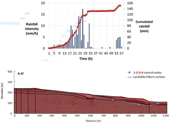
Figure 5.
Above, the plot of the rainfall intensity with time during the event that triggered the 2013 Montescaglioso landslide. Below, the seepage domain adopted for the SEEP/W transient analysis: discretization mesh and boundary conditions. The failure surface of the landslide is also reported, along with the location of the control nodes (1–4) used to follow the variation of the pore water pressures with time (see text for further details).
In the seepage analysis, a slope steady-state groundwater regime, representative of the ordinary hydraulic conditions in the slope, consistent with a water table at depth of about 10 m from the ground surface (Figure 5), was assumed to be the initial pore water pressure distribution. This is in accordance with the available well and open-pipe piezometer data. Then, a transient seepage analysis was simulated by assuming the event rainfall history as boundary condition along the slope surface, as shown in Figure 5. The permeability saturated coefficients of the different strata were prescribed according to the literature data available for the Sub-Apennine Clays [33,34]. In particular, the coefficient of permeability, ksat, for the lower unweathered grey was assumed to be equal to 4 × 10⁻⁸ m/s, whereas it was set at equal to slightly larger values for the upper layers in order to account for the weathering effects and the higher sand component (Table 1). As concerns the partially saturated soils above the water table, a coefficient of permeability constant with suction was assumed for the upstream layers’ soils, whereas a variation of the unsaturated coefficient of permeability with suction was taken into account for the other layers. For the latter, the variation of the volumetric water content with suction (soil–water characteristic curve) was estimated based on the grain size curve, according to the method suggested by Arya and Paris [38]; the law of variation of the unsaturated hydraulic conductivity with respect to suction was defined following Green and Corey [39].
An impervious boundary was assigned at the bottom of the mesh, whereas the actual rainfall intensity of the event, as reported in the sketch in Figure 5, was prescribed along the slope profile. A constant total head was assumed along both right and left boundaries of the seepage domain: in particular, at the right boundary, the value of the hydraulic head was set equal to the elevation of the water course at the toe of the slope, whereas it was imposed at 15 m depth below the ground level along the left boundary to comply with in situ measurements.
The results of the transient seepage analysis are reported in Figure 6 in terms of the variations of piezometric head calculated against time for four nodes of the mesh along the sliding surface (see points 1–4 in Figure 5), along with the variation of the cumulated rainfall with time.
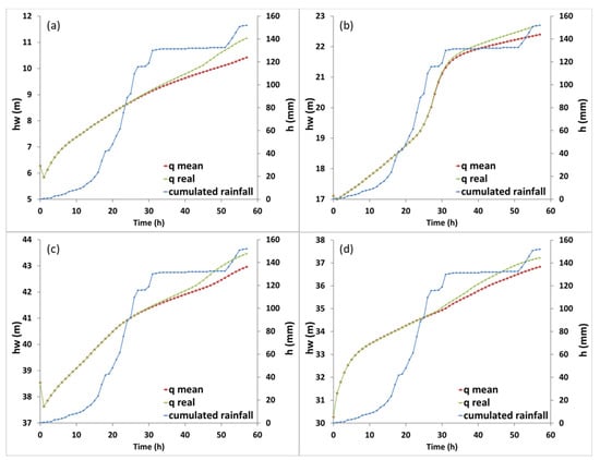
Figure 6.
Variation with time of the cumulated rainfall and pore water pressure resulting from the seepage analysis for Nodes 1 (a), 2 (b), 3 (c), and 4 (d). Node locations are shown in Figure 5.
The plots show that, in the first stage of rainfall infiltration (the first ten hours), the piezometric head values in the shallower nodes located within the conglomerates (Nos. 1 and 4) increase with rates higher than the nodes located at depth in the clay substratum (Nos. 2 and 3). Later on, Nodes 1 and 4 tend toward a steady increase of piezometric heads, whereas Node 2 is characterized by a larger increase of piezometric heads as an effect of the significant rainfall height cumulated during the 15–30 h time interval. The effect of such strong rainfall intensity in this latter time interval is also observed for all nodes in terms of a slightly delayed increase of piezometric heads calculated in the following hours. The overall variations of piezometric heads are in the order of 5–7 m, reaching the maximum value of 7 m at the toe of the slope (Node 4). In the same plots, the curves of piezometric heads obtained by assuming a constant average intensity for the whole rainfall time duration are reported for comparison. A slight difference is observed only in the last stage of the rainfall term.
The pore water pressure distributions obtained from the transient seepage analyses were then implemented in a time-dependent limit equilibrium analysis to assess the variation of the stability conditions of the landslide body during the event (Figure 7).
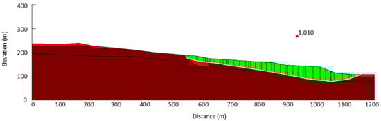
Figure 7.
Safety factor obtained in the LE analysis after 56 h from the beginning of the rainfall event.
Since the latter can be interpreted as a partial reactivation along a pre-existing sliding surface (see Section 1), the shear strength values adopted for the back-analysis of the clay layer were those at the residual (see Table 1). The whole set of material parameters adopted for the different layers is reported in Table 1, and the results are shown in Figure 8 in terms of the variation of safety factor values against time, along with the variation of cumulated rainfall height. The results of the time-dependent limit equilibrium analyses indicate that the safety factor starts from an initial value of 1.17, meaning quite stable conditions, and then reaches about unity at the end of the rainfall history after 56 h. A clear increase in the FS variation rate is observed after 25–30 h from the beginning of the rainfall event as a consequence of the strong increment of cumulated rainfall. It is interesting to note that the FS continues to decrease even after the accumulated rainfall reaches a plateau.
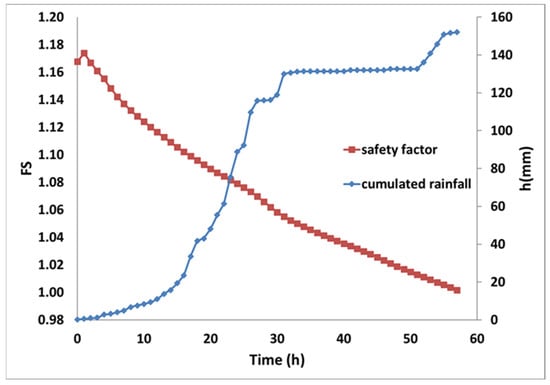
Figure 8.
Variation of the safety factor for the assumed landslide body, along with the cumulated rainfall data recorded during the event.
These results can provide a reasonable explanation for the landslide triggering, taking into account the permeability values for the soil materials assumed in the seepage analysis. Therefore, in this study, no effect of preferential seepage flows, water filling of tension cracks, or rear scarps in the crown area, as well as the potential effect of the rupture of the pipeline passing across the landslide body, was accounted for.
5. Three-Dimensional Finite Element Analysis
The evolution of the stress–strain state in the examined slope leading to the 2013 December landslide reactivation and the resulting displacement field were investigated also by means of a three-dimensional finite element analysis performed with PLAXIS-3D code [40].
In this analysis, the effects of a prescribed increase in the groundwater level, assumed in accordance with the results of the seepage analysis, on the reactivation of the landslide body were simulated. The 3D analysis was carried out using standard soil constitutive laws and taking into account the results of the geotechnical characterization of the soil materials described above. For the sake of simplicity, in this model, only two materials, i.e., sandy conglomerates and clays, were considered: therefore, the loose sand debris was included in the sandy conglomerates, while all clays were included in a single clay layer. A linear elastic perfectly plastic model with a Mohr–Coulomb strength criterion and a non-associated flow rule (ψ = 0°) was assumed for such materials, considering c′ = 100 kPa and ϕ′ = 28° as representative shear strength parameters for the conglomerates and c′ = 10 kPa and ϕ′ = 20° for the intact clays. Moreover, a pre-imposed planar layer was included in the clays to simulate the geometry of the assumed pre-existing shear band, for which strength parameter values corresponding to residual conditions (i.e., c′ = 0 and ϕ′ = 12°) were prescribed. The whole set of mechanical and hydraulic parameters used in the numerical simulation is reported in Table 2. From the Digital Elevation Model (DEM) in Figure 9, the 3D FEM model was built considering 85,222 tetrahedral elements. The mesh is coarser at the bottom and finer in the upper part of the domain. Two different pore pressure distributions were assigned in the simulations: (i) initial steady-state non-critical conditions; and (ii) post-rainfall critical conditions, i.e., corresponding to a water table very close to the ground surface.
Table 2.
Soil hydraulic and mechanical parameters adopted in the stress–strain FEM analyses.
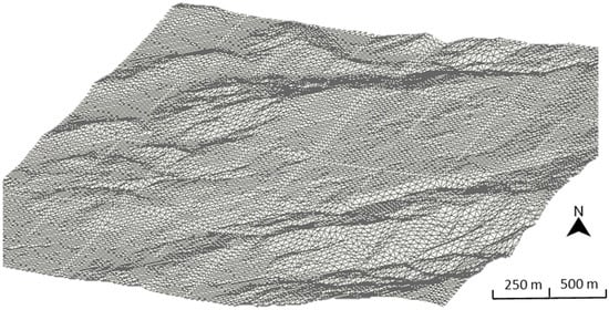
Figure 9.
DEM adopted for the construction of the 3D FEM model.
To simulate the pore pressure distribution representative of non-critical steady-state conditions, an impermeable boundary was assigned to the bottom of the mesh, whereas constant values of the groundwater head were prescribed along its vertical boundaries. Pore pressures equal to zero were imposed on the nodes corresponding to the stream at the toe of the slope, while free draining conditions were prescribed to the nodes at the ground surface. The resulting water table is approximately 10 m below ground level, except for the upper hillslope, where it reaches a depth of about 15 m. This steady-state water table is approximately consistent with the field data acquired in the slope during the post-event monitoring activity, which should also correspond to the pre-event water table conditions. The post-rainfall critical pore water pressure distribution was, instead, obtained by significantly increasing the hydraulic head value applied at the left-hand boundary, e.g., the top of the slope, in order to achieve a water table in agreement with that resulting from the transient seepage analysis (Section 4). The initial stress state in the slope was obtained by simulating a gravity loading procedure [41]. The stages of the analysis have progressively included the initial stress state assignment, the activation of the pre-existing shear band, and then the implementation of the critical pore water pressure distribution to simulate the effects of the rainfall event.
Under the non-critical steady-state pore-pressure regime and after the activation of the shear band, which means assuming residual parameters for the same layer, the slope became stable. Later on, the increment of pore water pressures within the slope, associated with post-rainfall critical condition, was simulated, and slope-instability conditions were found (also indicated by lack of numerical convergence) as a result of the concentration of plastic shear straining approximately in the portion of the shear band where the landslide area actually developed. In particular, the slope-failure mechanism seems to develop at the lower slope and then propagate according to a retrogressive mechanism. The calculated 3D displacement field is shown in Figure 10 in terms of the contours of horizontal displacement component along the y-axis and indicates that the largest horizontal displacement components are oriented along the y-axis and concentrate in the lower portion of the slope (orange and yellow zones), with values progressively lower in the upper slope.
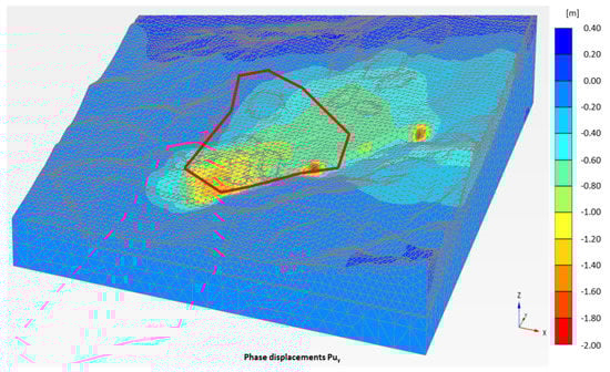
Figure 10.
Y−direction displacement contours.
This is in good agreement with the observed in situ failure mechanism and, in particular, with the direction of the larger horizontal displacement (N–S direction), as well as with the retrogressive evolution of the landslide process, as reconstructed by means of remote sensing and interferometry techniques [13,14,15,16,17,23]. Figure 11 reports the in situ vertical and horizontal displacement maps to highlight one of the aforementioned displacement fields, as reconstructed by Amanti et al. [23].
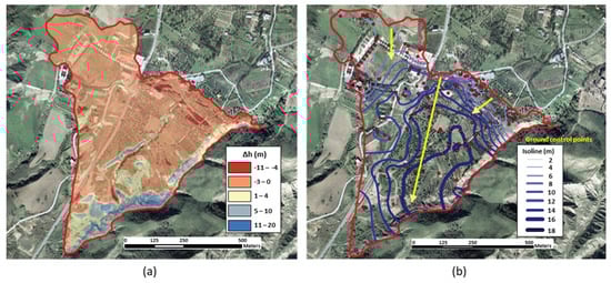
Figure 11.
(a) Vertical and (b) horizontal displacement maps reconstructed by comparing pre− and post−event orthophoto and LIDAR surveys (modified from [23]).
Actually, a significant uplift of the stream bed was measured in situ after the landslide reactivation, along with settlements of the ground surface in the uppermost sectors of the landslide area [14,15,17,23]. A longitudinal section of the deviatoric strain activated at failure can be seen in Figure 12. This shear straining is concentrated along the pre-imposed shear band and connects with the toe of the slope and the landslide crown through new shear zones, crossing areas not affected by previous straining.
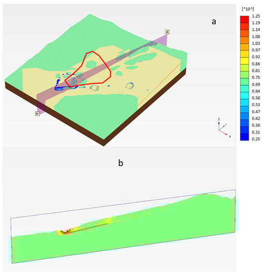
Figure 12.
Contours of the deviatoric strains calculated (a) and the cross−section of the landslide area (b).
6. Post-Failure Landslide Activity Monitoring
A topographic network consisting of a Robotized Total Station (RTS) and optical targets was installed to monitor the area of interest in the 2013 landslide, as well as to identify urban areas potentially affected by retrogressive landslide activities (Figure 13).
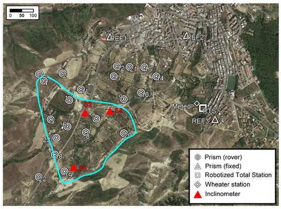
Figure 13.
Aerial view of the landslide area with the location of the topographic targets (white circles 1−23), the Robotized Total Station (RTS white square), and the inclinometers (S2, S6, S8 red triangles). The landslide limit is shown in the pale blue color. The fixed point is shown with white triangles (REF1, REF2, and REF3).
The RTS was set on a private terrace southeast of the town, with a view over the whole landslide and the lower part of Montescaglioso. In order to ensure the maximum measurement effectiveness, three fixed points (REF1, REF2, and REF3) were also installed in stable areas (cemetery, municipal auditorium, and sector behind the total station), so that accuracy of 1 cm in the planimetric and altimetric components was reached. The measured cumulated displacements are close to zero throughout the monitored area, even in the portion where large displacements occurred in 2013 (Figure 13 and Figure 14).
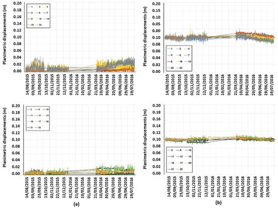
Figure 14.
Post-failure RTS displacement monitoring data for the landslide area (upper graphs) and the upslope area (lower graphs): (a) horizontal component and (b) vertical component.
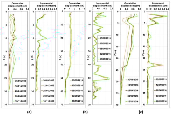
A post-failure inclinometer monitoring was also carried out within S2, S6, and S8 boreholes (Figure 1). The readings (Figure 15) indicate cumulated displacements that are generally below the accuracy level recognized for such instruments, also with a trend that does not suggest an evolution towards instability. Nonetheless, the inclinometer profiles show some clear bending at specific depths (51 m at S6, and 23 m at S8) that could correspond to the depth of the weakness zone or the shear band.
7. Concluding Remarks
The present paper discussed a detailed study of the December 2013 Montescaglioso landslide reactivation, which was triggered by an exceptional rainfall event and caused severe damage to structures and roads. This work aimed at interpreting the main triggering and aggravating factors that were responsible for the landslide instability and the high mobility of the slide mass. A detailed post-failure geomorphological analysis, an interpretation of a large geotechnical dataset on the soils involved, a time-dependent limit equilibrium analysis implementing the results of 2D transient seepage finite element analysis, and a 3D stress–strain finite element analysis were performed.
The limit equilibrium analysis provided useful indications on the variation of the slope safety factor during the rainfall event, whereas the transient seepage analysis allowed for the identification of a significant increase in pore water pressures induced by the rainfall even at large depths, i.e., where the shear band is supposed. According to the seepage analysis results, this phenomenon could be related to the high permeability of the materials overlying the clays, thus allowing for rapid infiltration of water at depth. The 3D numerical model allowed us to investigate the overall failure mechanism in terms of the extent of the unstable area, the evolution of the slope failure, and the soil strength mobilized along the shear band. Furthermore, it gave us an insight into the main landslide movement directivity and the areal distribution of displacement components; the latter resulted in a good agreement with the in situ landslide mobility, as reconstructed from geomorphological mapping, DTM surveys, and satellite interferometry analyses. Both analyses confirm that the mobilized strength of the soil is close to the residual value, and the failure process can be described as a reactivation of a portion of a pre-existing landslide shear band located in the deep clay layer.
On the basis of all analyses, the main factor that might be responsible for the rapid reactivation has to be found in the rapid increase of pore water pressures following the infiltration of the exceptionally large amount of rainfall. It has to be mentioned that other factors that were not investigated in the present work could have potentially played some roles in the landslide triggering and the consequent unexpectedly high displacement rate: among these, the breaking of an aqueduct pipeline crossing longitudinally the slide area, the rapid infiltration of runoff water within vertical fractures, and the brittleness associated with the development of new portions of the failure surface at the scarp area and in the toe region.
Author Contributions
P.L., conceptualization, data curation, investigation, methodology, and supervision; A.U., data curation and formal analysis; D.d.L., data curation and formal analysis; M.P., data curation and investigation; C.V., data curation and investigation; P.A., data curation and investigation; N.L.F., conceptualization, formal analysis, data curation, investigation, and methodology. All authors have read and agreed to the published version of the manuscript.
Funding
This research received no external funding.
Data Availability Statement
Not applicable.
Conflicts of Interest
The authors have no conflict of interest to declare that are relevant to the content of this article and have no relevant financial interest to disclose.
References
- D’Elia, B.; Picarelli, L.; Leroueil, S.; Vaunat, J. Geotechnical characterization of slope movements in structurally complex clay soils and stiff jointed clays. Ital. Geotech. J. 1998, 32, 5–32. [Google Scholar]
- Skempton, A.W.; Hutchinson, J. Stability of natural slopesand embankment foundations. In Proceedings of the Soil Mechanics and Foundation Engineering Conference Proceeding/Mexico/Berkshire, TRID, Mexico City, Mexico, 1969; pp. 291–340. [Google Scholar]
- Vaunat, J.; Leroueil, S.; Faure, R. Slope movements: A geotechnical perspective. In Proceedings of the International Congress International Association of Engineering Geology Lisbon, Lisbon, Portugal, 5 September 1994; pp. 1637–1646. [Google Scholar]
- Hutchinson, J.N. Mechanisms producing large displacements in landslides on pre-existing shears. Mem. Geol. Soc. China 1987, 9, 175–200. [Google Scholar]
- Herrada, M.A.; Gutiérrez-Martin, A.; Montanero, J.M. Modeling infiltration rates in a saturated/unsaturated soil under the free draining condition. J. Hydrol. 2014, 515, 10–15. [Google Scholar] [CrossRef]
- Brunetti, M.T.; Peruccacci, S.; Rossi, M.; Luciani, S.; Valigi, D.; Guzzetti, F. Rainfall thresholds for the possible occurrence of landslides in italy. Nat. Hazards Earth Syst. Sci. 2010, 10, 447–458. [Google Scholar] [CrossRef]
- Gutiérrez-Martín, A.; Ángel Herrada, M.; Yenes, J.I.; Castedo, R. Development and validation of the terrain stability model for assessing landslide instability during heavy rain infiltration. Nat. Hazards Earth Syst. Sci. 2019, 19, 721–736. [Google Scholar] [CrossRef]
- Gutiérrez-Martín, A. A GIS-physically-based emergency methodology for predicting rainfall-induced shallow landslide zonation. Geomorphology 2020, 359, 107121. [Google Scholar] [CrossRef]
- D’Ecclesiis, G.; Lorenzo, P. Frane relitte nei depositi della fossa bradanica: La frana di Madonna della Nuova (Montescaglioso, Basilicata). G. Geol. Appl. 2006, 4, 257–262. (In Italian) [Google Scholar]
- Cruden, D.M.; Varnes, D.J. Landslide types and processes. In Landslides: Investigation and Mitigation; Turner, A.K., Schuster, R.L., Eds.; Transportation Research Board: Washington, DC, USA, 1996; pp. 36–75. [Google Scholar]
- Parise, M.; Gueguen, E.; Vennari, C. Mapping surface features produced by an active landslide. IOP Conf. Ser. Earth Environ. Sci. 2016, 44, 022029. [Google Scholar] [CrossRef]
- Pellicani, R.; Spilotro, G.; Ermini, R.; Sdao, F. The large Montescaglioso landslide of December 2013 after prolonged and severe seasonal climate conditions. In Landslides and Engineered Slopes. Experience, Theory and Practice; Aversa, S., Cascini, L., Picarelli, L., Scavia, C., Eds.; CRC Press: Boca Raton, FL, USA, 2016; Volume 3, pp. 1591–1597. [Google Scholar]
- Pellicani, R.; Argentiero, I.; Manzari, P.; Spilotro, G.; Marzo, C.; Ermini, R.; Apollonio, C. UAV and airborne LiDAR data for interpreting kinematic evolution of landslide movements: The case study of the Montescaglioso landslide (Southern Italy). Geosciences 2019, 9, 248. [Google Scholar] [CrossRef]
- Manconi, A.; Casu, F.; Ardizzone, F.; Bonano, M.; Cardinali, M.; De Luca, C.; Gueguen, E.; Marchesini, I.; Parise, M.; Vennari, C.; et al. Rapid mapping of event landslides: The 3 December 2013 Montescaglioso landslide (Italy). NHESS 2014, 14, 1835–1841. [Google Scholar]
- Raspini, F.; Ciampalini, A.; Del Conte, S.; Lombardi, L.; Nocentini, M.; Gigli, G.; Ferretti, A.; Casagli, N. Exploitation of amplitude and phase of satellite SAR images for landslide mapping: The case of Montescaglioso (South Italy). Remote Sens. 2015, 7, 14576–14596. [Google Scholar] [CrossRef]
- Caporossi, P.; Mazzanti, P.; Bozzano, F. Digital Image Correlation (DIC) analysis of the 3 December 2013 Montescaglioso landslide (Basilicata, Southern Italy): Results from a multi-dataset investigation. ISPRS Int. J. Geo-Inf. 2018, 7, 372. [Google Scholar] [CrossRef]
- Lazzari, M.; Piccarreta, M. Landslide disasters triggered by extreme rainfall events: The case of Montescaglioso (Basilicata, Southern Italy). Geosciences 2018, 8, 377. [Google Scholar] [CrossRef]
- Bozzano, F.; Caporossi, P.; Esposito, C.; Martino, S.; Mazzanti, P.; Moretto, S.; Scarascia Mugnozza, G.; Rizzo, A.M. Mechanism of the Montescaglioso landslide (Southern Italy) inferred by geological survey and remote sensing. In Advancing Culture of Living with Landslides: Volume 2 Advances in Landslide Science; Springer International Publishing: Cham, Switzerland, 2017. [Google Scholar]
- Nian, T.K.; Huang, R.Q.; Wan, S.S.; Chen, G.Q. Three-dimensional strength-reduction finite element analysis of slopes: Geometric effects. Can. Geotech. J. 2012, 49, 499–511. [Google Scholar] [CrossRef]
- Troncone, A.; Conte, E.; Donato, A. Two and three-dimensional numerical analysis of the progressive failure that occurred in an excavation-induced landslide. Eng. Geol. 2014, 183, 265–275. [Google Scholar] [CrossRef]
- De Novellis, V.; Castaldo, R.; Lollino, P.; Manunta, M.; Tizzani, P. Advanced three-dimensional finite element modeling of a slow landslide through the exploitation of DInSAR measurements and in situ surveys. Remote Sens. 2016, 8, 670. [Google Scholar] [CrossRef]
- Lollino, P.; Giordan, D.; Allasia, P.; Fazio, N.L.; Perrotti, M.; Cafaro, F. Assessment of post-failure evolution of a large earthflow through field monitoring and numerical modelling. Landslides 2020, 17, 2013–2026. [Google Scholar] [CrossRef]
- Amanti, M.; Chiessi, V.; Guarino, P.M.; Spizzichino, D.; Troccoli, A.; Vizzini, G.; Fazio, N.L.; Lollino, P.; Parise, M.; Vennari, C. Back-analysis of a large earth-slide in stiff clays induced by intense rainfalls. In Landslides and Engineered Slopes. Experience, Theory and Practice, Proceedings of the 12th International Symposium on Landslides, Naples, Italy, 12–19 June 2016; Aversa, S., Cascini, L., Picarelli, L., Scavia, C., Eds.; CRC Press: Boca Raton, FL, USA, 2016. [Google Scholar]
- Pieri, P.; Tropeano, M.; Sabato, L.; Lazzari, M.; Moretti, M. Quadro stratigrafico dei depositi regressivi della Fossa bradanica (Pleistocene) nell’area compresa fra Venosa e il Mar Ionio. J. Geol. 1998, 60, 318–320. [Google Scholar]
- Ricchetti, G. Alcune osservazioni sulla serie della Fossa Bradanica. Le “Calcareniti di M. Castiglione”. Boll. Soc. Nat. Napoli 1965, 75, 3–11. [Google Scholar]
- Boenzi, F.; Radina, B.; Ricchetti, G.; Valduga, A. Note Illustrative della Carta Geologica d’Italia alla scala 1:100,000 del Foglio 201 “Matera”. Serv. Geol. Ital. 1971, 48. [Google Scholar]
- Bonardi, G. Carta Geologica Dell’Appennino Meridionale, 1:250,000; CNR: Roma, Italy, 1988. [Google Scholar]
- Pieri, P.; Sabato, L.; Tropeano, M. Significato geodinamico dei caratteri deposizionali e strutturali della Fossa bradanica nel Pleistocene. Mem. Soc. Geol. Ital. 1996, 51, 501–515. [Google Scholar]
- Sabato, L. Quadro stratigrafico-deposizionale dei depositi regressivi nell’area di Irsina (Fossa bradanica). Geol. Romana 1996, 32, 219–230. [Google Scholar]
- Tropeano, M.; Sabato, L.; Pieri, P. Filling and cannibalization of a foredeep: Bradanic Trough, southern Italy. Geol. Soc. Lond. Spec. Publ. 2002, 191, 55–79. [Google Scholar] [CrossRef]
- Cotecchia, V. Geotechnical vulnerability and geological evolution of the Middle Adriatic coastal environment. Ital. Geotech. J. 1999, 3, 46–55. [Google Scholar]
- Cafaro, F.; Cotecchia, F. Structure degradation and changes in the mechanical behaviour of a stiff clay due to weathering. Geotechnique 2001, 51, 441–453. [Google Scholar] [CrossRef]
- Lollino, P.; Cotecchia, F.; Zdravkovic, L.; Potts, D.M. Numerical analysis and monitoring of Pappadai dam. Can. Geotech. J. 2005, 42, 1631–1643. [Google Scholar] [CrossRef]
- Lollino, P.; Santaloia, F.; Amorosi, A.; Cotecchia, F. Delayed failure of quarry slopes in stiff clays: The case of the Lucera landslide. Géotechnique 2011, 61, 861–874. [Google Scholar] [CrossRef]
- Di Maio, C.; Vassallo, R. Geotechnical characterization of a landslide in a Blue Clay slope. Landslides 2011, 8, 17–32. [Google Scholar] [CrossRef]
- Geostudio. Seep/W and Slope/W Reference Manual; Geostudio: Calgary, AB, Canada, 2012; Available online: https://www.geoslope.com/learning/support-resources#dnn_BooksHeaderPane (accessed on 2 March 2023).
- Morgenstern, N.R.; Price, V.E. The analysis of the stability of general slip surfaces. Geotechnique 1965, 15, 79–93. [Google Scholar] [CrossRef]
- Arya, L.M.; Paris, J.F. A Physico-empirical Model to Predict the Soil Moisture Characteristic from Particle-Size Distribution and Bulk Density Data. Soil Sci. Soc. Am. J. 1981, 45, 1023–1030. [Google Scholar] [CrossRef]
- Green, R.E.; Corey, J.C. Calculation of hydraulic conductivity: A further evaluation of some predictive methods. Soil Sci. Soc. Amer. Proc. 1971, 35, 3–8. [Google Scholar] [CrossRef]
- PlaxisBV. PLAXIS-3D. Reference Manual; PlaxisBV: Delft, The Netherlands, 2014; Available online: https://communities.bentley.com/products/geotech-analysis/w/wiki/46137/manuals---plaxis (accessed on 2 March 2023).
- Griffiths, D.V.; Lane, P.A. Slope stability by finite elements. Géotechnique 1999, 49, 387–403. [Google Scholar] [CrossRef]


Disclaimer/Publisher’s Note: The statements, opinions and data contained in all publications are solely those of the individual author(s) and contributor(s) and not of MDPI and/or the editor(s). MDPI and/or the editor(s) disclaim responsibility for any injury to people or property resulting from any ideas, methods, instructions or products referred to in the content. |
© 2023 by the authors. Licensee MDPI, Basel, Switzerland. This article is an open access article distributed under the terms and conditions of the Creative Commons Attribution (CC BY) license (https://creativecommons.org/licenses/by/4.0/).