Abstract
Punta Licosa promontory is located in the northern part of the Cilento coast, in the southern Tyrrhenian basin. This promontory is bordered by sea cliffs connected to a wide shore platform sloping slightly towards the sea. This area has been considered stable at least since Late Pleistocene, as testified by a series of evidence well known in the literature. The aim of this research is to reconstruct the main coastal changes that have occurred in this area since the middle Holocene by means of the literature data, aerial photo interpretation, satellite images, GPS measurements, direct underwater surveys, GIS elaborations of high-resolution DTMs, bathymetric data and high-resolution orthophotos taken by UAV. Particular attention was paid to the wide platform positioned between −7.2 ± 1.2 m MSL and the present MSL, this being the coastal landform interpreted as the main consequence of sea cliff retreat. The elevation of this landform was compared with the GIA models calculated for the southern Tyrrhenian area, allowing establishing that it was shaped during the last 7.6 ± 1.1 ky BP. Moreover, the interpretation of archaeological and geomorphological markers led to the reconstruction of the shoreline evolution of this coastal sector since 7.6 ky BP. This research evaluates the cliff retreat under the effect of Holocene RSL variation on Cilento promontories, located in the western Mediterranean and characterised by the presence of monophasic platforms, and the applied method can be considered more effective and less complex and expensive if compared to other effective approaches such as those based on the usage of cosmogenic nuclides.
1. Introduction
Since the historical time, coastal areas have represented the most vulnerable geomorphic environments, subject to the combined effects of both coastal and terrestrial processes, and they are still one of the most anthropized and developed zones worldwide [1,2,3,4]. Coastal environments are characterised by numerous coastal landforms (i.e., shore platforms, coastal spit, tidal flats, etc.) and, in turn, characteristics of rocky or sandy coasts. Among these different environments, here we focus our attention on rocky coasts (sensu Kennedy et al. [5]), intended as erosional environments related to the landward retreat of the cliffs at the shoreline.
Even if sandy coasts represent the most dynamic and studied environments, affected by an immediate response of the coastal system to the sea-level oscillations, rocky coasts represent a substantial part of the world’s coastlines, constituting 53% of the coast in the central Mediterranean area, where more than 41% of the regional population lives near the coast [6].
Rocky coasts tend to evolve by retreating due to wave action. Their morpho evolution is strictly connected to RSL changes in response to global sea-level variations, glacio-hydro-isostatic adjustments (GIA), and vertical ground movements (VGMs) related to regional and local tectonics. Hundreds of years are necessary to shape a decametric shore platform [7,8,9,10] when prolonged sea-level stands or slow sea-level change rates occur.
Both the emerged and submerged parts of rocky coasts can be sculptured by different evidence of ancient sea-level stands [8,11,12,13], providing important information about former paleo-sea levels. In turn, by comparing these data with Holocene GIA models, the main tectonic behaviour of a specific coastal sector can be assessed in detail by applying statistical approaches [14]. In addition, such a comparison could also be effective for evaluating the retreat rates of sea cliffs.
Among erosional coastal landforms suitable as sea-level markers (SLMs), shore platforms [15,16,17,18] are considered high-precision sea-level index points (SLIPs) as they form between the high and low tidal levels [19,20], and are the most important evidence of cliff retreat mainly depending on the balance between the geological properties of the bedrock and the marine forcing during a period of RSL stand or slow RSL rise [8,10,21,22,23,24]. In addition, if cut on a less erosive substrate, shore platforms can preserve their morphology over thousands of years.
Along the Mediterranean coast, numerous pieces of evidence of these erosional landforms have resulted from the combined effects of sea-level changes and tectonic uplift [25,26] in both emerged and submerged areas [27,28]. However, due to the complexity of operative theatre, only recently has the development of innovative techniques made it possible to obtain high-resolution mapping of the seabed [27] and the following geomorphological interpretation of the underwater paleo-shore platforms as evidence of Holocene sea cliff retreat trends [10,29].
As regards the central-Tyrrhenian coast, several studies dealing with the recent and historical evolution of rocky coasts allowed the measuring of the average retreating rates of sea cliffs associated with shore platforms, such as the case of Campanian tuff coasts, where cliff retreat rates of 0.04 m/y were evaluated for the last sixty years [30,31,32]. In the case of Procida volcanic island, the submerged area was investigated to analyse a large number of depositional and erosional submerged surfaces in order to identify the controlling factors which may have affected their distribution during the Holocene [10,33,34,35].
Moving southward on the Cilento coast (Campania region, southern Italy), even if several studies allowed the recognition of well-defined Middle to Upper Pleistocene emerged marine terraces [36,37,38,39,40], none of them have been focused on the present-day shore platforms, which may provide relevant information concerning the evolutionary coastal trends in the area.
This research aims to reconstruct the coastal response to Holocene sea-level rise in the part of Cilento promontory where the shore platforms are better exposed (Punta Licosa), through a multi-temporal and multi-technic geomorphological analysis with particular attention paid to the evaluation of sea cliff retreat and shore platform formation over the last 8.0 ky. To fulfil such objectives, a morphometric analysis of the present-day emerged and submerged platform and related cliff was applied to a detailed Digital Terrain Model (DTM), obtained by using a multi-technic approach including acoustic and optical methods. The fact that the study area has been considered tectonically stable by different previous studies [41,42] has enabled the neglect of the influence of the tectonic component on the RSL variation.
2. Geological and Meteo-Marine Settings
Punta Licosa Promontory is located in the southern part of the Campania Region (southern Italy) between Castellabate Plain and Ogliastro Bay, and it extends over 10 km [43], covering an area of about 4.12 km2. The emerged part of the promontory falls in the Cilento and Vallo di Diano National Park, while the submerged part belongs to the Protected Marine Area of Santa Maria di Castellabate due to its great environmental and scenic value [44].
From a geological point of view, the promontory is mainly composed of Quaternary units (Figure 1) grouped into four geological formations which are, starting from the oldest one, the Pollica Sandstones (Langhian), the San Mauro Formation (Langhian, Lower Tortonian), the Valle del Lambro Synthem (Middle Pleistocene) and the Palinuro Synthem (Upper Pleistocene) [45], and alluvial fan deposits (Upper Pleistocene, Holocene). The submerged part is mainly characterised by an undifferentiated terrigenous substratum (Mesozoic tertiary) and by Holocene outer shelf deposits.
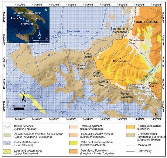
Figure 1.
(A): Location map of the study area (B): geological map of the Punta Licosa promontory with the chronological classification of the main geological units (modified from Martelli et al. [45]).
Pollica Sandstones and the San Mauro Formation belong to the Cilento Group [45] and are both constituted by arenaceous-pelitic turbidites. In particular, while Pollica Sandstones have a main siliciclastic component, the San Mauro Formation is mainly characterised by marly-calcarenite composition with conglomeratic intervals [46,47].
The terrains of Valle del Lambro Synthem are mainly terraced deposits formed by alternating lenses of imbricated fluvial gravels, whereas the deposits of the Palinuro Synthem are mainly formed by bioclastic calcarenites in the lower part and cross-laminated sands in the upper part [37,48]. A few metres above the present riverbed of the Rio Dell’Arena, Holocene terraced alluvial deposits occur. The latter are mainly represented by heterogeneous, incoherent and heterometric deposits, made mainly of gravels and sands. The analysed, submerged part is mainly characterised by an undifferentiated terrigenous substratum, represented by tertiary siliciclastic and carbonate terrains mainly attributed to the Cilento group (especially Pollica sandstones). Occasionally, it is possible to observe a Pleistocene sand bank mainly composed of coarse organogenic sands with fragmented and/or intact shells. Late Holocene Outer shelf deposits are represented by medium-fine sands with bio and lithoclasts rich in rhyzomes of marine phanerogams and pelites.
In the inlets of the promontory and in Castellabate and Ogliastro plains, recent beach deposits are recognisable. These deposits are constituted by medium-thin, coarse, gravelly sands, and sandy gravels with heterometric stones, coarse up to arenitic blocks, modelled by the modern marine currents.
The main tectonic structures, and the most evident at the scale of the outcrop, are mainly N–S extensional faults (Figure 1) showing vertical and transcurrent evidence of movements. In particular, the major tectonic structure consists of a deformation band characterised by brittle deformation that runs from San Marco di Castellabate to Agnone, in a WNW–ESE direction; this structure splits into multiple faults towards the southeast. In San Marco di Castellabate, a fault parallel to this zone of deformation, probably a lower-order structure, drops down the Tyrrhenian calcarenites [45].
This area is characterised by a Mediterranean temperate climate with average annual temperatures of 17° (12.6–20.8°), characterised by an average annual rainfall of 729.7 mm [44], mainly concentrated in spring and late autumn, and long periods of drought during the summer. The area has a mainly semidiurnal microtidal regime, with maximal ranges of ca. ± 0.6 m and a minimum range of about −0.1 m [49] during spring tides, while during neap tide oscillations are weaker [50].
Generally, waves with the highest significant height (exceeding 6 m) come from the SW sector [51]. This is also the direction containing the maximum geographical sea fetch, with a maximum value exceeding 800 km.
3. Materials and Methods
In this study, a multi-technical approach including direct and indirect methods was applied in order to obtain a detailed characterisation of both the emerged and submerged sectors of the study area. In particular, data from detailed direct surveys were overlaid by those coming from indirect surveys, such as photo-interpretation, morphometric analysis of high-resolution DTMs from Lidar and bathymetric data, and analysis of morpho-acoustic and optical data measured with different instruments, supported by an accurate literature review of previous works.
All the adopted methodologies are summarised in the diagram shown in Figure 2.
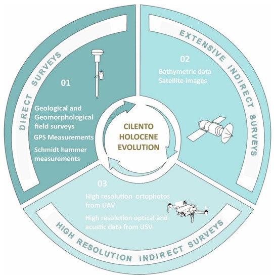
Figure 2.
Flowchart describing the methodological approach used in this research.
Particular attention was paid to the seabed investigation through different kind of bathymetric surveys [52] aimed at reconstructing the submerged morphologies located in the shallow water sector, whose morphometric analysis provided clear evidence of the Holocene coastal modification and parallel retreat.
Various methods can be used for bathymetric surveys, including multi-beam echosounder (MBES) and single-beam echosounder (SBES) surveys, based on the principle of acoustic wave propagation in water. In fact, a single-beam device includes a transducer combining transmitter and receiver that sends a sound pulse straight down into the water; the signal reaches the seabed, where it is reflected or refracted, and a part of it returns to the transducer; computers measure the time interval between the transmission and reception of the sound pulse precisely [53,54,55], knowing the sound velocity of the water using one of the empirical available formulas [56].
Unlike single-beam, multi-beam uses a series of sound pulses from the transmitter to scan a large swath of the seabed beneath the ship, across the track. The appropriate processing of the footprints of data from the irradiated footprints can give the water depth values of hundreds or even more measured points on the seabed in the vertical plane perpendicular to the course, so that accurate and rapid measurements can be made [57,58,59,60,61,62]. The scan angle is fixed, so the swath width depends on the depth of the water: the deeper the depth, the wider the swath; consequently, several track lines are necessary in shallow waters to completely cover the survey area.
It is also possible to quantify the backscatter of the sound signal that is computed by measuring the amount of sound reflected by the sea floor and received by the instrument [63,64] so to achieve information about bottom hardness, roughness and types (e.g., rock, mud, etc.).
However, the use of ships equipped with acoustic survey devices is difficult in specific remote and not easily accessible areas, such as in shallow water where the ship is at risk and materials can be lost. Alternative technologies such as remotely operated vehicles (ROVs) and/or unmanned surface vehicles (USVs) are also used to acquire bathymetric data bypassing the obstacles of the execution of traditional bathymetric survey techniques in difficult areas [65,66,67].
Remote sensing makes it possible to investigate, also for bathymetric purposes, areas that are difficult to access without high costs [68,69]. Using imagery techniques, depths can be determined quickly over large remote coastal areas, and also in presence of dangerous hazards, submerged objects and steep seabed morphology [70]. The use of remotely sensed images for generating bathymetric depths has been investigated since the 1970s, as testified by the study carried out by the University of Michigan for the Spacecraft Project of the US Naval Oceanographic Office [71]. However, Satellite-Derived Bathymetry (SDB) has had a strong development in recent years, also due to the wide availability of remotely sensed images with increasingly high geometric resolution. The accuracy of SDB maps is partly a function of water clarity, depth, and wave climate [72]. SDB is suitable for achieving depth in shallow coastal areas, but at present the results do not reach the accuracy of traditional bathymetric surveys, such as single-beam and multi-beam [73].
Within a remote sensing approach to explore bathymetry in shallow water, another instrument capable of measuring the depth of the sea is Laser Imaging Detection and Ranging (LIDAR), which uses light in the form of a pulsed laser to measure ranges (variable distances) to the investigated surface [74]. The most widely used platforms on which a LIDAR system is employed are airplanes and helicopters.
Bathymetric data can be also be easily extracted from digital nautical charts available in raster and vector form. In particular, the vector files include depth points and isolines that are easily selectable and directly usable for interpolation method applications to generate 3D bathymetric models [75]. The interpolation of sea depth values derived from nautical charts is certainly the simplest approach to obtain a continuous bathymetric model of the desired area, but the data available are sometimes not updated and do not present the desired level of detail (small or medium scale rather than a large scale of representation).
Taking into account the strengths and weaknesses of the different bathymetry acquisition techniques, a good compromise can be reached by integrating data from different sources, paying, however, particular attention to the different accuracy levels. In particular, updated nautical charts were not available for our study area (that is, the Tyrrhenian coast around Punta Licosa (Italy)) so the existing ones did not provide adequate support for the morphological study. For this reason, we used recently acquired depth data to build a 3D bathymetric model. We also experimented with SDB techniques deriving bathymetry from 2022 satellite images.
By using this approach, a morphological reconstruction of the Punta Licosa coast was carried out, providing a detailed mapping of the shore platform and evaluating the cliff retreat rate over the last 7.6 ky.
3.1. Geological and Geomorphological Field Surveys and GPS Measurements
The main direct surveys carried out in this study included geological and geomorphological field observations aimed at recognising all the morphologies and main indicators of paleo-sea level stands located in the emerged and transitional coastal area. In addition, sea–land sections were traced using GNSS R6 Trimbles to precisely characterise the main morphological variations.
3.2. Schmidt Hammer Measurements
In order to define the rock mass quality characterising the cliffs and estimate their mechanical properties, ‘non-destructive’ field investigations were carried out on the emerged part of the cliff face. The instrument used to evaluate uniaxial compressive strength (UCS) was the Schmidt hammer (or sclerometer) model ECTHA 1000. The operating principle of this instrument means that a mass shot from a spring impacts a plunger in contact with the surface of the rock and the test result is expressed in terms of the rebound distance of the mass. The hammer is pressed on the rock wall using an orientation of choice, normally preferring a vertically downward orientation where possible, and a rebound number on the Schmidt hammer is recorded [76].
In each selected site, about 20 readings must be recorded, discarding the highest and lowest values according to the procedure suggested by the ISRM (International Society for Rock Mechanics) [77]. Knowing the density of the tested rock and the rebound number, it is possible to determine the UCS.
3.3. Photogrammetric Surveys and Post-Processing
Low-flying Unmanned Aerial Vehicles (UAVs) were used to obtain detailed and high-resolution images along the rocky promontory [78,79]. This survey technique needs to define a flight plan for covering the entire area of interest with a suitable set of photos. Specifically, it is necessary to set a sufficient overlap (about 80%) between two adjacent images and the flight altitude in order to obtain the desired GSD (Ground Sample Distance). The GSD is the size assumed by the pixel on the terrain; a smaller GSD indicates higher spatial resolution and more detailed imagery, while a larger GSD indicates lower resolution and less detail. GSD is an important parameter for defining the potential spatial resolution of a point cloud generated by photogrammetric algorithms.
Images were acquired during low tide using a UAV (DJI Phantom 4) flying about 40 m above the sea cliff and the shore platforms to obtain a mean GSD (Ground Sample Distance) of less than 5 cm. Flights were carried out in October 2021, and in April and June 2022 (further details are reported in Table 1).

Table 1.
Image acquisition data.
Before the image acquisition, several photogrammetric targets were located in the area of interest, both on the land surface and on the sea bottom. Such targets were made of soft PVC in order to be easily transportable. Ballast must be used during installation to prevent any movement caused by sea movement or wind. These targets are typically designed with easily detectable features in images, such as high-contrast markings and distinctive shapes. In this work, classic 75 cm square Survey Aerial Targets (SATs) were used, whose high contrast was ensured by the Iron Cross pattern, in which the target area is divided into four quadrants coloured alternatively in black and yellow.
A specialised operator placed the photogrammetric targets on the area of interest by following the instructions below reported:
- Each target was placed on the ground (or sea bottom) by employing ballasts or stakes;
- The spatial arrangement of targets was chosen to cover the entire area of interest, and the configuration sought to be in accordance with Von Gruber spatial arrangement [80];
- They were placed so that their location was visible in the images and easily accessible with a GNSS receiver.
For each survey, at least three targets were positioned on the sea bottom at different depths, 0.5, 1.0 and 1.5 m, and their position was estimated using the geodetic multi-constellation GNSS receiver Leica Leica-GS15.
The UAV data were then processed in the laboratory by using the Agisoft Metashape software. The images were elaborated and filtered to remove overexposed images, erroneous data and damaged files, and were processed, using Structure from Motion (SfM) algorithms [81,82] to obtain a 3D Point Cloud useful for extracting geomorphological information into three dimensions. The GNSS data were processed in PPK (Post Processing Kinematic) mode in order to obtain an accuracy comparable with the GSD. The targets were used as Ground Control Points (GCPs) to constrain the 3D model to a specific reference system and to contain the model deformations. The targets located on the seabed were used to estimate the water refraction effect, which modifies the height of the underwater points [83]. Finally, a unique high-precision Digital Elevation Model (DEM) covering the submerged part and the shore was produced. Moreover, using the DEM, an orthoimage and a GeoTIFF of the area of interest were produced.
3.4. ARGO Surveys and Post-Processing
In order to carry out indirect geophysical surveys in the accessible shallow water sectors characterised by the presence of shore platforms, a USV called ARGO was applied. This catamaran-like platform, with a length of 1.20 m and a width of 0.86 m, was used in order to collect high-precision data on the seabed morphology, precisely map the main underwater geomorphological features, and test the data obtained from the UAV surveys. In particular, ARGO is a technological project of marine drones, designed and engineered in 2020 in the laboratories of Parthenope University, aimed at testing an innovative methodology for geological and geomorphological marine investigations in shallow water sectors, usually considered critical areas to be investigated by using traditional survey boats [66,84,85,86].
The USV is powered by two T-200 thrusters with three-blade propellers on brushless motors which provides a 2-knot data acquisition speed. The unmanned equipment is furnished with acoustic and optical sensors integrated through innovative technological approaches [84,85]. The geo-acoustic sensors are:
- (i)
- A single-beam echo sounder (SBES, Ohmex SonaLite) with 200 kHz acquisition frequency, with a depth range of 0.3–80 m and an accuracy of 0.025 m;
- (ii)
- A sides scan sonar (SSS; Sonar Tritech Side-Scan StarFish 450C) optimised for coastal waters (450 kHz CHIRP transmission) with a slant range between 1 and 100 m each channel and a maximum precision under optimal water conditions of 0.0254 m. During the survey, the SSS range was 30 m and, in the case of the Punta Ogliastro site, two lines with an 80% overlap were carried out.
These instruments were embedded in the USV with an offset of a few centimetres from the GPS (Global Positioning System). The optical sensors consisted of two Xiaomi YI Action cameras placed parallel to the vertical axis, with a variable stereoscopic base chosen based on the bathymetry of the study area and a GoPro Hero 3 forming an angle of about 30 with the seabed. All the acquired data were transmitted in broadcasting, allowing the simultaneous work of a multidisciplinary team of specialists able to analyse specific datasets in real time.
The acquired SSS data were processed by using Chesapeake Sonar Web Pro 3.16 software to create a GeoTIFF mosaic and obtain the sonar coverage of the surveyed areas. In the case of the Punta Ogliastro site, the mosaic had a resolution of 0.1 × 0.1 m. The interpretation of the mosaic, by means of backscattering analysis, allowed discrimination between sandy and rocky bottoms [66,87]. This analysis was confirmed by comparing the mosaic with the georeferenced photos recorded by the photogrammetric system.
The GIS (Geographic Information System) analysis of the data allowed the mapping of seabed landforms, classified through the backscattering analysis.
3.5. Satellite Images and Post-Processing
Sentinel-2 images and depth data were used to experiment with another technique for obtaining a digital bathymetric model (DBM) of the study area. Downloaded from the Copernicus platform [88], the images were acquired on 21 July 2022 and generated as 2A processing level products to represent the Bottom of Atmosphere (BOA) reflectance; in fact, they were derived from Level-1C products using algorithms of scene classification and atmospheric correction [89]. The dataset includes 13 multispectral bands with different geometric resolutions. In particular, the two bands used to generate the bathymetric model, specifically Blue and Green Bands, both present a resolution of 10 m.
In order to obtain the DBM, the Bands Ratio Method (BRM) was applied using Blue and Green bands [90] with a 3rd-degree polynomial (3DP) [91]. This method requires knowing the depth at some points to define the relationship between band ratio values and depth values. Depth data were extracted from the HD sonar bathymetric chart (SBC), derived from the Navionics website [92]. SBCs were created by using Navionics proprietary systems that process sonar data contributed by boaters with existing content derived from multiple official nautical charts, government and private sources. Specifically, 80 depth points were selected along a transect located in the central part of the investigated area, and developed perpendicularly to the coastline so as to investigate the variability of depth proceeding offshore. Once the image pre-processing phase had been carried out and the relationship between reflectance values and depth values established, a DBM of the area was obtained with the same resolution as the Sentinel-2 used images (10 m).
To test the accuracy of the bathymetric model, since the depth points and contour lines are available on the Navionics website, the differences (residuals) were found between the nautical chart depth values and the corresponding ones in DBM. We calculated statistics, i.e., minimum, maximum, mean, standard deviation and Root Mean Square Error (RMSE), of those residuals. The following formula was used to calculate RMSE:
where µ is the mean value of the residuals and σ is the standard deviation.
The model obtained, therefore, appears to be reliable up to a depth of 25 m because it presents in this zone residuals with RMSE equal to 2.77 m. The greatest error values are recorded in the bordering areas of the most peripheral bathymetric lines (i.e., 30 m), with a maximum value equal to the pixel size (10 m). Particularly, the accuracy is better near the coast; in fact, the model in the 0–5 m depth range has an RMSE value of 0.905 m.
3.6. Spatial Analysis and Data Elaboration
All data collected were processed in the GIS environment (ArcGIS 10.4) in order to obtain an emerged-submerged DTM.
In particular, the emerged DTM was obtained from the LIDAR data provided by the Ministry of the Environment and Energy Safety (Ministero dell’Ambiente e della Sicurezza Energetica, MASE), which through a topographic survey of the Italian territory mapped part of the nation. The MASE provides, in the national geoportal, the DTMs in raster format with different resolutions (1 m × 1 m, 2 m × 2 m and 20 m × 20 m); in our study the 2 m × 2 m one was used, ranging between 0 and +300 m MSL, with a planimetric accuracy of approximately 30 cm and 15 cm in height [93].
As regards the submerged area, depth data were obtained by means of the SDB procedure described in the previous sub-section.
3.6.1. Morphometric Analysis
The submerged landforms identified in the study area were interpreted as shore platforms through the integration of different sources of data and according to the following criteria:
- i.
- Morphometric analysis of satellite images;
- ii.
- Morphometric analysis of extension, borders and slope from the high-resolution DTMs and related reclassification into three classes (sub-horizontal surfaces between 0 and 5%; gently sloping surfaces between 5 and 15%; steep slopes greater than 15%);
- iii.
- Morpho-structural analysis of the coastal sector by in situ surveys;
- iv.
- Analysis of the geological data available for the submerged sector of the study area where the rocky seabed is identified [45];
- v.
- Analysis of bibliographic seismo-stratigraphic data regarding the definition of lithology and the orientation of the strata [26,44];
- vi.
- Definition of the primary process forming the surface.
3.6.2. Analysis of Meteo-Marine Data
In order to obtain a quantitative evaluation of the above-mentioned morphological responses, a careful meteo-marine analysis was carried out. Wave data records analysed in this study were supplied by the Italian SeaWave Measurement Network [94] and recorded between 07 January 1989 and 31 December 2014 (3 h sampling rate with some data gaps) by an ondametric buoy located near the island of Ponza (40°52′00.10” N, 12°56′60.00′′ E), at a nominal depth of 115 m, which belongs to the Italian National Tide gauge network. This buoy was chosen as it is the ondameter closest to the study area, and because it records the longest available time series of meteo-marine data to allow the reconstruction of the effect of wave action on the sea cliffs along the analysed coastal sector [10].
A dataset made of a total of 74,519 wave records was downloaded, containing information regarding significant wave height (Hs), wave period (T), and mean wave direction (Dm). These data were processed to improve the information on the wave climate representative of the central-southern Tyrrhenian Sea already provided by Di Luccio et al. [95].
The sea states registered by the wave buoy were subdivided into 7 meteo-marine classes based on the significant wave height value (i.e., a: Hs ≤ 1; b: 1 < Hs ≤ 2; c: 2 < Hs ≤ 3; d: 3 < Hs ≤ 4; e: 4 < Hs ≤ 5; f: 5 < Hs ≤ 6; g: Hs > 6). This subdivision was performed for all events in the series, and a rose diagram was created for each direction (as shown in Figure 9 of the Section 4).
One of the focuses of this analysis was the evaluation of geographical fetch, i.e., the maximum extension of the areas potentially subject to the direct action of the wind. Then, these data were compared to the effective fetch, i.e., the distance over which the wind can travel across the open water, by using the following equations from Saville [96] and Seymour [97]:
where Fe,w is the effective fetch length relative to direction Φw, Fi is the length of the geographical fetch relative to the i-th direction Φi, Φw is the average direction referring to the geographical north of the possible origin of the wind responsible for the wave motion generation, Φi is the i-th direction referring to the geographical north related to a sector of 2𝜃 considered around Φw (Φw–𝜃 ≤ Φi ≤ Φw + 𝜃), 𝜃 is the width of the sector of the possible wave motion origin, with an estimated value of ± 45° and ± 90° according to Saville’s and Seymour’s methods, respectively, and n is an exponential term defined according to the law of directional distribution of the wave spectra that characterise the study area (generally estimated as n = 2).
Finally, we compared the fetch values with the prevalent wave height to establish the influence of the most significant parameters.
3.7. Procedure for the Evaluation of the Retreating Rates
The study area was divided in different sectors according to their exposure to wave fronts. For each sector, a series of transects 50 m distant from each other were produced in order to evaluate the retreating rates (RR) that affected the platform in the considered time span by using the following equation:
where Exti are the n measurements of extension taken for each platform with a 50 m step, and ΔT is the time period in years in which the platforms remained active.
In a further step, the error related to this value was evaluated through the following equation:
where RRmax represented the highest value of Retreat rate evaluated while RRmin represent the lowest one.
3.8. GIA Models and RSL Data
According to several authors [8,98], a shore platform can be interpreted as SLIP by detecting two particular morphological elements (Figure 3) on its surface, represented by the outer margin (i.e., the termination point of the platform towards the sea), related to the sea-level position at the beginning of the platform formation (time T1 in Figure 3), and the inner margin (i.e., the contact point between the horizontal bedrock and the vertical rocky cliff), related to the sea-level position at the end of the platform formation (or present-day MSL in the case of active landforms; time T2 in Figure 2).
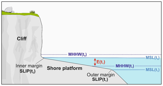
Figure 3.
Shore platform as sea-level index point (SLIP).
Both inner and outer margins, at the moment of their formation, are located at the same level as the mean higher high water (MHHW, i.e., average of the higher high water height of each tidal day observed over a Tidal Datum Epoch) that in the study area is equal to 0.25 m. Consequently, the SLIP associated with this indicator can be calculated as follows:
where E is the elevation of the platform at issue concerning the former mean sea level (MSL). In this research, we assumed that MHHW(t1) had the same value as MHHW(t2).
SLIP = E − MHHW
Generally, if the inner and/or outer margin of a shore platform is not precisely detectable, the medium altitude of the landform can be interpreted as a marine limiting point (MLP, sensu Vacchi et al. [13]), helping in the assessment of a lower limit for the former RSL position. Furthermore, in order to interpret these landforms as SLIP or MLP, it is necessary to date them through absolute (i.e., radiocarbon dating technique) or relative methods (i.e., indirect chronological correlations).
In this study, the outer margin of the shore platform was detected by overlaying data from GPS measurements, satellite images analysis and UAV and USV surveys.
Regarding its dating, a new indirect procedure has been proposed based on the comparison between the altimetric position of this landform and a series of GIA models specifically created for the study area [99].
This suite of RSL curves was produced by using the sea-level equation solver SELEN [100], coupled with three ice-sheet models [101,102,103]. The sea-level equation was solved for a total of 54 models, assuming different values for both the lithosphere thickness and the lower and intermediate mantle viscosity.
4. Results
All the performed analyses led to the characterisation of the present-day shore platform along the whole coastal sector by integrating previous data with the new data derived from the performed direct and indirect surveys.
4.1. Characterisation, Geomechanical Proprieties and Morphometric Analysis of the Cliff Rocks (Emerged Area)
The physical and mechanical characterisation was performed on the lithologies belonging to Pollica sandstones in which both the present-day sea cliffs and the related shore platforms are shaped. The rocks from this formation are arenaceous-pelitic turbidites, predominantly silicoclastics with medium to fine arenites. These sandstones are moderately altered and characterised by the presence of discontinuities spaced at more than 6 cm. In addition, from field survey observations, the strata layering on the cliff face gently dip landwards for almost the entire promontory.
Keeping in mind the density of these rocks, of about 2.30 × 10³ kg/m3, values of UCS between 58 and 60 and 70 MPa were calculated in all the sites (Table 2) with the exception of the San Marco di Castellabate site, made of highly fractured cemented sands, for which lower values were estimated. All the values obtained in each site are listed in Table 2.
Table 2.
Obtained UCS values along the Licosa promontory.
Moreover, GPS measurements were carried out along the whole coastal sector in order to observe the main topographic variations, measure the height of the inner margin of the present-day shore platform and assess the height of the cliffs along the study area (Table 3).
Table 3.
GPS measurements obtained along the Punta Licosa Promontory.
4.2. Morphometric Analysis of the Submerged Area and RSL Determination
The first result of this integrated analysis was the detailed mapping of the present-day shore platform all around the Punta Licosa promontory, between San Marco di Castellabate in the north, and Punta Ogliastro in the south (Figure 4). This was achieved by integrating the morphometric analysis with on-field surveys and the study of cartographic and seismo-stratigraphic sources, in accordance with the methodology previously described (see Section 3.6.1).
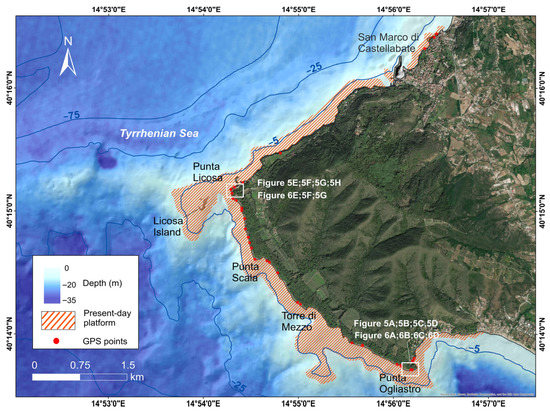
Figure 4.
Distribution of the present-day platform along the Punta Licosa promontory. The DTM of the submerged sector is derived from satellite image analysis.
In particular, while the majority of the platform’s morphology was reconstructed through the analysis of satellite images, Punta Ogliastro and Punta Licosa (Figure 5), located in the southern and central part of the promontory, respectively, were surveyed in detail by using UAVs and USVs devices. These sites were considered strategic due to the fact that along their coasts the platform is well-exposed and visible, allowing its detailed geomorphological characterisation (Figure 5 and Figure 6).
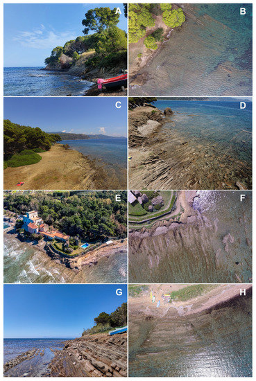
Figure 5.
Detail of the two sites investigated through UAV Survey: (A–D) Punta Ogliastro; (E–H) Punta Licosa. Location is shown in Figure 4.
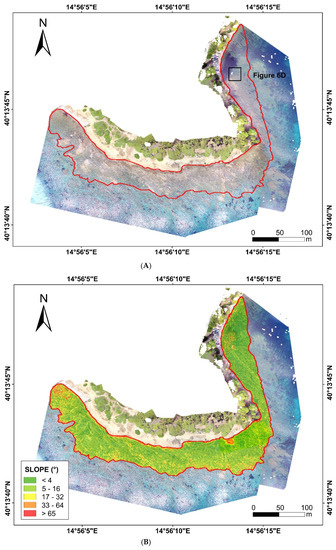
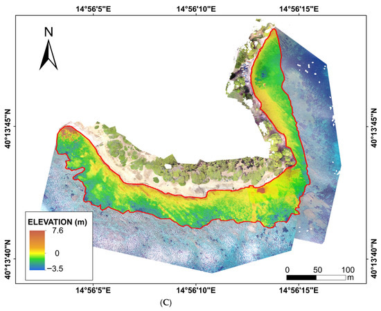
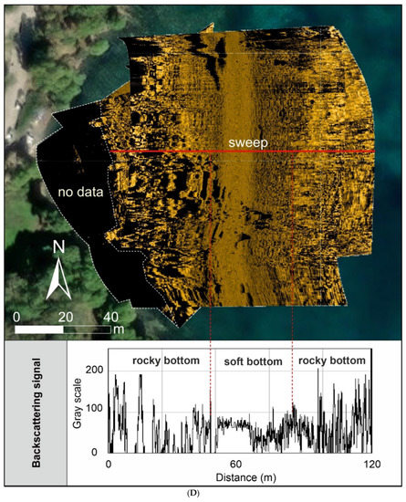
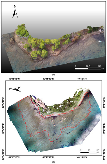
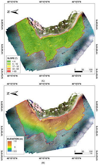
Figure 6.
Main characteristics of the Punta Ogliastro site: (A) investigated platform; (B) slope in degrees; (C) elevation in meters; (D) Side Scan Sonar analysis; (E) dense cloud of the emerged and submerged part of the Punta Ogliastro rocky coast. Main Features of Punta Licosa site: (F) investigated platform; (G) slope in degrees; (H) elevation in meters.
For both platforms, the reconstruction of the emerged-submerged DEM was performed together with a slope analysis in the GIS environment and the related re-classification into four reference classes according to Gomez-Pazo et al. [104].
According to data, the UAV-surveyed portion of the platform at Punta Ogliastro (Figure 5A–D and Figure 6E) is characterised by a width of approximately 20 m and an along-shore length of 100 m, covering a total area of 15.976 m2 (Figure 6A), with an elevation ranging between 0 m and −3.5 m m.s.l. (Figure 6C) and the presence of some emerged blocks reaching 1.3 m m.s.l. At Punta Ogliastro, the analysis of the high-resolution slope map of the platform (Figure 6B) allowed its classification as a sub-horizontal surface, with the definition of its main inclination generally lower than 4°, and the detection of micro-morphologies on the surface characterised by higher slope values ranging between 33° and 64°, with local peaks over 65°. These dome morphologies are characteristic of differential erosion happening on structures characterised by the presence of different layers, where the easiest erodible lithologies are removed by the wave action, forming flatter surfaces, in favour of the hardest ones, resulting in the formation of gibbous morphologies. In more detail, the flattest and most homogenous sector of the platform appears to be the eastern one, characterised by an N–S orientation, followed by the frontal sector, with an E–W orientation, characterised by a higher local slope variability. By contrast, the western sector of the platform, with a NNW–SSE orientation, shows the most numerous pieces of evidence related to differential erosion. Additionally, in the case of Punta Ogliastro, the integration between the morphometric analysis and acoustic data calibrated through the comparison with georeferenced videos allowed seabed classification. In particular, the backscattering analysis along a sweep (Figure 6D) demonstrated that the highest backscattering values (200–255 in greyscale) were associated with the rocky bottom (which reflected 78–100% of the acoustic signal emitted by the SSS transducer). Instead, values lower than 100 can be associated with an area covered by soft sediments (reflecting at maximum 50% of the acoustic signal). The signal variability (0–255) associated with the rocky seafloor can be interpreted as evidence of the roughness due to the erosive effects, in accordance with the image analysis from georeferenced videos. Otherwise, the analysed part of the platform at the Punta Licosa site (Figure 5D–G) showed a width and an along-shore length of about 76.5 m and 414 m, respectively, covering an area of 30.430 m2 (Figure 6F) with an elevation ranging between 0 m and −3.5 m m.s.l. (Figure 6H) and some emerged areas reaching 1.8 m m.s.l. In this case, the analysis of the high-resolution slope map of the platform (Figure 6G) allowed assessing that more than 95% of the platform as characterised by a main inclination generally lower than 4°, with higher local slope values almost absent, consequently classifying it as sub-horizontal surface. In more detail, by analysing the map in Figure 6G it is possible to observe that the minor slope variations are characterised by a NO–SE orientation, according to the direction of the layers and following the contact between the most and least erodible lithologies. As previously described for the case of Punta Ogliastro, this conformation is also related to differential erosion by wave action.
Moving on to the extensive analysis of the submerged sector of the study area, the platform at issue, with its outer margin positioned between −6.0 m MSL and −8.4 m MSL, showed a quite irregular shape (i.e., spatial extension variability) in the different parts of the promontory and, based on its exposure to wave action, was divided into four sectors ranging from PL1 to PL4 (Figure 7).
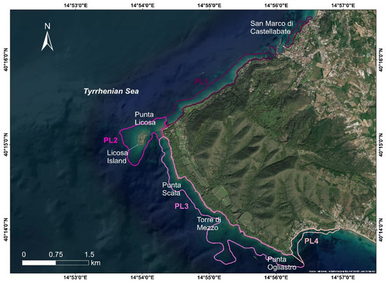
Figure 7.
Division of the Punta Licosa Promontory into four coastal sectors (PL1 to PL 4) based on their exposure to the wave action.
The widest detected platform is located along the central part of the promontory (PL2 sector, see Figure 7 for location) and reaches a maximum extension of 905 m in its central part. This area corresponds to the elongation of Punta Licosa and Licosa Island, located about 360 m from the coast.
However, in the northern part of the promontory, along the PL1 sector (see Figure 7 for the location), the active shore platform shows a maximum extension of 282 m. Moving towards the southern part of the promontory, along the PL3 sector (see Figure 7 for the location), the platform shows a maximum extension of 610 m while, in the southernmost part of the promontory, in the correspondence of Ogliastro Bay and the PL4 sector (see Figure 7 for the location), the platform shows its minimum size with a maximum extension of about 170 m.
Finally, considering the tectonic stability of the study area assessed by previous studies [41,42], the correlation between the position of the outer margin platform, identified as the beginning of the erosional phase, and the available GIA models specifically produced for the area [99] allowed the estimation of the period for the formation of the platform between 8.7 and 6.5 ky BP (Figure 8), in correspondence with the Holocene slow-down of the RSL rise. Consequently, a SLIP at 7.2 ± 1.2 m was calculated and chronologically constrained to 7.6 ± 1.1 ky BP, considering the average value of the time span associated with the platform’s formation.
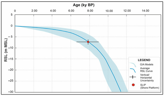
Figure 8.
The RSL data derived from the Holocene shore platforms and the GIA predictions for the Gulf of Naples [99].
4.3. Retreat Rates Evaluations
Another fundamental result obtained from our multi-technique approach to the study of a tectonically stable coastal sector was the precise measuring of the sea cliffs’ retreat rates by applying a morphometric analysis to our high-resolution DTMs derived from the satellite image elaboration coupled with a detailed analysis of UAV and USV DTMs.
The analysis was made, characterising each block, ranging from PL1 to PL4 (see Figure 6 for location), obtaining sea-cliff retreat rates which differed from sector to sector (Table 4) according to the procedure described in the Section 3. In particular, the highest average retreat rates (RRs med) of 0.072 and 0.034 m/y were observed in the central part of the promontory, along the PL2 and PL3 sectors, respectively (Table 4). The lowest RRs med of 0.023 and 0.014 m/y were observed in the northern and southern parts of the promontory, along the PL1 and PL3 sectors, respectively.
Table 4.
Maximum (RRs max), minimum (RRs min) and average (RRs med) retreat rates for the four sectors of the Punta Licosa Promontory (PL1, PL2, PL3, PL4).
Retreat values differed despite the overall geological and lithological uniformity of the studied coast, as also demonstrated by comparable values of UCS obtained through Schmidt hammer measurements. In some cases, the only difference observed in the geological configuration during our direct and indirect surveys was related to the dipping of strata. This allows the exclusion of lithological or tectonic reasons for the significant variations in erodibility.
Therefore, to define the possible influence of offshore/nearshore waves along the Licosa promontory on sea cliff retreat rates, the acquired data about the general and local wave climate were examined.
The highest waves approach the coast from SW. Maximum wave heights exceeded 6 m off PL2 and PL3 sectors, and about 5.5 m off PL1 and PL4 sectors (Figure 9).
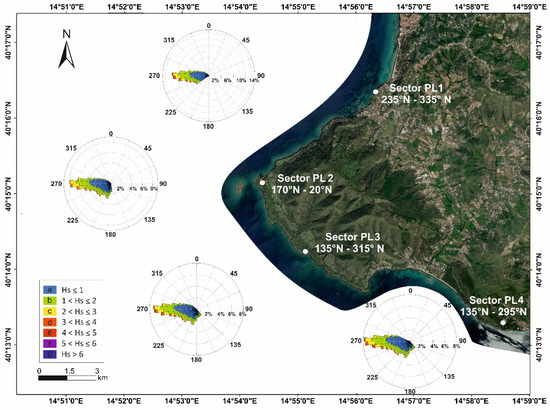
Figure 9.
Significant wave height roses obtained for PL1-PL4 sectors.
In particular, the PL1 sector showed exposure to wave events, mainly coming from 235 to 335°N (SW/NW). As is clearly visible from the rose diagram related to this sector (Figure 9), the higher percentage of events occurring in this sector belonged to classes a and b of wave height (i.e., Hs ≤ 1 and 1< Hs ≤ 2), respectively, representing 64.5% and 24.0% of the total events occurring in the coastal sector. On the other hand, the events belonging to the classes e, f and g (i.e., Hs ≥ 4 m) represented 0.6% of the total events. The highest geographical fetch of this sector was measured between 230° N and 245° N, with a length of more than 500 km, while the effective fetch referring to 245° N was equal to 179 km.
PL2 is an open coastal sector exposed to the dominant SW–NW waves. In fact, the reported rise diagram shows that the occurrence direction of waves ranged between 180° N and 300° N. This is also the direction from which 100% of waves with a significant wave height above 3 m occurred (Classes of Hs d; e; f; g), which represents 0.53% of the total events. SW–NW is also the occurrence direction of events belonging to class a and b of Hs, representing 65.5% and 23.8% of the total events, respectively. The highest geographical fetch of this sector was measured between 230° N and 250° N, with a length of about 900km, while the effective fetch referring to 250° N was equal to 580 km.
The PL3 sector faces the direction of the SW–W swells but is sheltered from more northerly waves, showing exposure to wave events from 135° N to 300° N. The highest percentage of events occurring in this coastal sector belonged to classes a and b of wave height, representing, respectively, 64.8% and 24.3%. The highest geographical fetch was measured at about 250° N with a length of about 900 km, while the effective fetch referred to this direction was equal to 600 km.
Finally, the PL4 sector showed exposure to wave events mainly coming from 135° N to 280° N and was largely sheltered from the main NW swells. The rise diagram related to this direction shows that the highest percentage of events that occurred in this coastal sector belonged to classes a and b of wave height, which, respectively, represented 63.8% and 24.8% of the total. The highest geographical fetch of this sector was measured between 250° N and 260° N with a length of more than 500 km, while the effective fetch referred to 255° N was equal to 260 km.
5. Discussion
The research at issue has studied for the first time the morpho-evolution of the present-day shore platform cut into sandstones along the Cilento coast.
In more detail, the performed multi-technical geomorphological analyses led to a full morphometric characterisation of the emerged and transitional rocky coast of Punta Licosa and the definition of the sea cliff response to the Holocene RSL changes. The overlap between multidisciplinary techniques and the realization of several direct and indirect surveys (i.e., SSS, USV, and UAV analysis) allowed the realisation of detailed mapping of the present-day platform otherwise impossible to achieve.
The platform was initially mapped at a large scale by using the DTM derived from the analysis of satellite images, and then carefully mapped through the use of UAV and USV surveys in those areas characterised by easy access and good water visibility, assessing the morphometry of this platform.
The morphological characterisation of the active shore platform, together with the determination of its outer margin position related to an RSL chronologically constrained by available GIA models, can be considered an effective result for the study area. In this way, the beginning of the shore platform formation was constrained at about 7.6 ± 1.1 ky BP, therefore evaluating the retreating trend occurred in the considered time span for the PL1–PL4 sectors.
By looking at the data reported in Table 3, it is possible to observe that the calculated retreat rates slightly differ and, considering the overall lithological uniformity of the coast, this behaviour may be ascribed to local wave climate variation.
In fact, the PL2 sector, which was characterised by the maximum extension of the platform and by the highest RR (RRmax 0.104 m/y), was also the sector most frequently exposed to waves with a height higher than 2m. Conversely, sector PL4 presented the lowest extension of the platform and the lowest value of RRmax (0.020 m/y) as a response to the lowest exposure to wave events.
The detailed geomorphological characterisation of the Holocene shore platform in this tectonically stable context allowed us to interpret this platform as a high-precision RSL marker indirectly dated through the correlation with the available sito-specific GIA models. Nevertheless, the integration between direct and indirect surveys provided crucial information on the response of this coastal system to the Holocene RSL change by evaluating the variation of the retreating rates.
6. Conclusions
Punta Licosa is one of the most attractive coastal landscape in southern Italy, being part of the Protected Marine Area of Santa Maria Di Castellabate. It represents a great example of a coast cut in sandstone lithologies whose evolution was not particularly influenced by anthropic pressure, and therefore it is a suitable area for those analyses aimed at evaluating the interplay between glacio-hydro-isostatic sea-level rise and coastal retreat rates.
This study underlines the importance of detailed and extensive assessments of the rocky coast response to sea-level changes. The interplay between large- and small-scale analysis allowed the reconstruction of the Holocene evolution, which was crucial for the characterisation of the present-day shore platform, making it possible to obtain the retreat rates of the coastal area since 7.6 ky BP.
Despite the proposed approach needing the availability of reliable and site-specific GIA models, in the case of a monophasic platform like those taken into account in the present work, it can be considered effective and less complex and expensive than some other effective approaches such as those based on the usage of cosmogenic nuclides [105,106].
Author Contributions
G.M., M.F.T. and C.C. designed the study and participated in all phases. S.D.P., C.P., C.M.R. and P.P.C.A. provided a global structural discussion and participated in the development of the methodological approach. M.F.T., C.C., S.D.P., A.M.A., G.M. and F.G.F. carried out the fieldwork observations and analysed the results. S.D.P., C.P., P.P.C.A., G.M., C.C. and M.F.T. made contributions regarding the conceptual approach. All authors have read and agreed to the published version of the manuscript.
Funding
This research received no external funding.
Data Availability Statement
Data are available within the article.
Acknowledgments
The authors sincerely thank Francesco Peluso, Luigi De Luca and Andrea Gionta for their contribution during the field and marine surveys.
Conflicts of Interest
The authors declare no conflict of interest.
Abbreviations
The following abbreviations are used in the manuscript:
| ALB | Airborne Laser Bathymetry |
| BOA | Bottom Of Atmosphere |
| DBM | Digital Bathymetric Model |
| DEM | Digital Elevation Model |
| DTM | Digital Terrain Model |
| GCP | Ground Control Points |
| GIA | Glacio-Hydro-Isostatic Adjustments |
| GIS | Geographic Information System |
| GNSS | Global Navigation Satellite System |
| GPS | Global Positioning System |
| GSD | Ground Sample Distance |
| LIDAR | Laser Imaging Detection and Ranging |
| MHHW | Mean Higher High Water |
| MLP | Marine Limiting Point |
| MSL | Medium Sea Level |
| NIR | Near InfraRed |
| NOAA | National Oceanic and Atmospheric Administration |
| PPK | Post Processing Kinematic |
| RMSE | Root Mean Square Error |
| ROV | Remotely Operated Vehicle |
| RSL | Relative Sea Level |
| SAT | Survey Aerial Target |
| SBES | Single-Beam Echo Sounder |
| SDB | Satellite-Derived Bathymetry |
| SfM | Structure from Motion |
| SLIP | Sea-Level Index Point |
| SLM | Sea-Level Marker |
| SSS | Side Scan Sonar |
| UAV | Unmanned Aerial Vehicle |
| UCS | Uniaxial Compressive Strength |
| USV | Unmanned Surface Vehicle |
References
- Aucelli, P.; Caporizzo, C.; Cinque, A.; Mattei, G.; Pappone, G.; Stefanile, M. New insight on the 1st century bc paleo-sea level and related vertical ground movements along the Baia—Miseno coastal sector (Campi Flegrei, Southern Italy). In Proceedings of the IMEKO TC4 International Conference on Metrology for Archaeology and Cultural Heritage; MetroArchaeo, Florence, Italy, 4–6 December 2019; Volume 2019, pp. 474–477. [Google Scholar]
- Aucelli, P.P.C.; Mattei, G.; Caporizzo, C.; Cinque, A.; Amato, L.; Stefanile, M.; Pappone, G. Multi-proxy analysis of relative sea-level and paleoshoreline changes during the last 2300 years in the Campi Flegrei caldera, Southern Italy. Quat. Int. 2021, 602, 110–130. [Google Scholar] [CrossRef]
- Caporizzo, C.; Gracia, F.J.; Aucelli, P.P.C.; Barbero, L.; Martín-Puertas, C.; Lagóstena, L.; Ruiz, J.A.; Alonso, C.; Mattei, G.; Galán-Ruffoni, I.; et al. Late-Holocene evolution of the Northern Bay of Cádiz from geomorphological, stratigraphic and archaeological data. Quat. Int. 2021, 602, 92–109. [Google Scholar] [CrossRef]
- Tursi, M.F.; Anfuso, G.; Matano, F.; Mattei, G.; Aucelli, P.P.C. A Methodological Tool to Assess Erosion Susceptibility of High Coastal Sectors: Case Studies from Campania Region (Southern Italy). Water 2023, 15, 121. [Google Scholar] [CrossRef]
- Kennedy, D.M.; Stephenson, W.J.; Naylor, L.A. Introduction to the rock coasts of the world. Geol. Soc. Lond. Mem. 2014, 40, 1–5. [Google Scholar] [CrossRef]
- Budetta, P.; Santo, A.; Vivenzio, F. Landslide Hazard Mapping along the Coastline of the Cilento Region (Italy) by Means of a GIS-Based Parameter Rating Approach. Geomorphology 2008, 94, 340–352. [Google Scholar] [CrossRef]
- Kanyaya, J.I.; Trenhaile, A.S. Tidal Wetting and Drying on Shore Platforms: An Experimental Assessment. Geomorphology 2005, 70, 129–146. [Google Scholar] [CrossRef]
- Rovere, A.; Raymo, M.E.; Vacchi, M.; Lorscheid, T.; Stocchi, P.; Gomez-Pujol, L.; Harris, D.L.; Casella, E.; O’Leary, M.J.; Hearty, P.J. The Analysis of Last Interglacial (MIS 5e) Relative Sea-Level Indicators: Reconstructing Sea-Level in a Warmer World. Earth Sci. Rev. 2016, 159, 404–427. [Google Scholar] [CrossRef]
- Mattei, G.; Aucelli, P.P.C.; Caporizzo, C.; Rizzo, A.; Pappone, G. New geomorphological and historical elements on morpho-evolutive trends and relative sea-level changes of Naples coast in the last 6000 years. Water 2020, 12, 2651. [Google Scholar] [CrossRef]
- Aucelli, P.P.; Mattei, G.; Caporizzo, C.; Di Luccio, D.; Tursi, M.F.; Pappone, G. Coastal vs Volcanic Processes: Procida Island as a Case of Complex Morpho-Evolutive Response. Mar. Geol. 2022, 448, 106814. [Google Scholar] [CrossRef]
- Evelpidou, N.; Pirazzoli, P.; Vassilopoulos, A.; Spada, G.; Ruggieri, G.; Tomasin, A. Late Holocene Sea Level Reconstructions Based on Observations of Roman Fish Tanks, Tyrrhenian Coast of Italy. Geoarchaeology 2012, 27, 259–277. [Google Scholar] [CrossRef]
- Lambeck, K.; Rouby, H.; Purcell, A.; Sun, Y.; Sambridge, M. Sea Level and Global Ice Volumes from the Last Glacial Maximum to the Holocene. Proc. Natl Acad. Sci. USA 2014, 111, 15296–15303. [Google Scholar] [CrossRef] [PubMed]
- Vacchi, M.; Marriner, N.; Morhange, C.; Spada, G.; Fontana, A.; Rovere, A. Multiproxy Assessment of Holocene Relative Sea-Level Changes in the Western Mediterranean: Sea-Level Variability and Improvements in the Definition of the Isostatic Signal. Earth Sci. Rev. 2016, 155, 172–197. [Google Scholar] [CrossRef]
- Stocchi, P.; Spada, G. Influence of Glacial Isostatic Adjustment upon Current Sea Level Variations in the Mediterranean. Tectonophysics 2009, 474, 56–68. [Google Scholar] [CrossRef]
- Davidson-Arnott, R.G. Rates of Erosion of till in the Nearshore Zone. Earth Surf. Process. Landf. 1986, 11, 53–58. [Google Scholar] [CrossRef]
- Sunamura, T. Geomorphology of Rocky Coasts; Wiley: New York, NY, USA, 1992. [Google Scholar]
- Trenhaile, A.S. Rock Coasts, with Particular Emphasis on Shore Platforms. Geomorphology 2002, 48, 7–22. [Google Scholar] [CrossRef]
- Bird, E. Coastal Cliffs: Morphology and Management; Springer: Berlin, Germany, 2016. [Google Scholar]
- Trenhaile, A.S. The Geomorphology of Rock Coasts; Oxford University Press: Oxford, UK, 1987. [Google Scholar]
- Trenhaile, A.S. Predicting the Response of Hard and Soft Rock Coasts to Changes in Sea Level and Wave Height. Clim. Chang. 2011, 109, 599–615. [Google Scholar] [CrossRef]
- Kennedy, D.M.; Dickson, M.E. Lithological Control on the Elevation of Shore Platforms in a Microtidal Setting. Earth Surf. Process. Landf. 2006, 31, 1575–1584. [Google Scholar] [CrossRef]
- Trenhaile, A.S.; Porter, N.J. Can Shore Platforms Be Produced Solely by Weathering Processes? Mar. Geol. 2007, 241, 79–92. [Google Scholar] [CrossRef]
- Trenhaile, A.S.; Kanyaya, J.I. The Role of Wave Erosion on Sloping and Horizontal Shore Platforms in Macro-and Mesotidal Environments. J. Coast. Res. 2007, 23, 298–309. [Google Scholar] [CrossRef]
- Murray-Wallace, C.V.; Woodroffe, C.D. Quaternary Sea-Level Changes: A Global Perspective; Cambridge University Press: Cambridge, UK; New York, NY, USA, 2014. [Google Scholar]
- Amato, V.; Aucelli, P.P.C.; Mattei, G.; Pennetta, M.; Rizzo, A.; Rosskopf, C.M.; Schiattarella, M. A geodatabase of Late Pleistocene-Holocene palaeo sea-level markers in the Gulf of Naples. Alp. Mediterr. Quat. 2018, 31, 5–9. [Google Scholar]
- Savini, A.; Bracchi, V.A.; Cammarosano, A.; Pennetta, M.; Russo, F. Terraced Landforms Onshore and Offshore the Cilento Promontory (South-Eastern Tyrrhenian Margin) and Their Significance as Quaternary Records of Sea Level Changes. Water 2021, 13, 566. [Google Scholar] [CrossRef]
- Micallef, A.; Krastel, S.; Savini, A. Introduction. In Submarine Geomorphology; Micallef, A., Krastel, S., Savini, A., Eds.; Springer: Berlin/Heidelberg, Germany, 2017. [Google Scholar]
- Casalbore, D.; Falese, F.; Martorelli, E.; Romagnoli, C.; Chiocci, F.L. Submarine Depositional Terraces in the Tyrrhenian Sea as a Proxy for Paleo-Sea Level Reconstruction: Problems and Perspective. Quat. Int. 2017, 439, 169–180. [Google Scholar] [CrossRef]
- Caporizzo, C.; Aucelli, P.P.C.; Di Martino, G.; Mattei, G.; Tonielli, R.; Pappone, G. Geomorphometric analysis of the natural and anthropogenic seascape of Naples (Italy): A high-resolution morpho-bathymetric survey. Trans. GIS 2021, 25, 2571–2595. [Google Scholar] [CrossRef]
- Aucelli, P.; Cinque, A.; Mattei, G.; Pappone, G. Historical Sea Level Changes and Effects on the Coasts of Sorrento Peninsula (Gulf of Naples): New Constrains from Recent Geoarchaeological Investigations. Palaeogeogr. Palaeoclimatol. Palaeoecol. 2016, 463, 112–125. [Google Scholar] [CrossRef]
- Caputo, T.; Marino, E.; Matano, F.; Somma, R.; Troise, C.; De Natale, G. Terrestrial Laser Scanning (TLS) Data for the Analysis of Coastal Tuff Cliff Retreat: Application to Coroglio Cliff, Naples, Italy. Ann. Geophys. 2018, 61, SE110. [Google Scholar] [CrossRef]
- Esposito, G.; Salvini, R.; Matano, F.; Sacchi, M.; Troise, C. Evaluation of Geomorphic Changes and Retreat Rates of a Coastal Pyroclastic Cliff in the Campi Flegrei Volcanic District, Southern Italy. J. Coast. Conserv. 2018, 22, 957–972. [Google Scholar] [CrossRef]
- Aucelli, P.P.C.; Gagliardi, E.; Mattei, G.; Napolitano, F.; Pappone, G.; Pennetta, M.; Tursi, M.F. Morphological responses to relative sea-level changes along Procida coast (Gulf of Naples, Italy) during the last 6.5 Ky. In Proceedings of the 2020 IEEE International Workshop on Metrology for the Sea (MetroSea), Napoli, Italy, 5–7 October 2020; IEEE: Piscataway, NJ, USA, 2020; pp. 175–179. [Google Scholar]
- Budillon, F.; Amodio, S.; Contestabile, P.; Alberico, I.; Innangi, S.; Molisso, F. The Present-Day Nearshore Submerged Depositional Terraces off the Campania Coast: An Analysis of Their Morpho-Bathymetric Variability. In Proceedings of the 2020 IEEE International Workshop on Metrology for the Sea (MetroSea), Napoli, Italy, 5–7 October 2020; IEEE: Piscataway, NJ, USA, 2020; pp. 132–138. [Google Scholar]
- Budillon, F.; Amodio, S.; Alberico, I.; Contestabile, P.; Vacchi, M.; Innangi, S.; Molisso, F. Present-Day Infralittoral Prograding Wedges (IPWs) in Central-Eastern Tyrrhenian Sea: Critical Issues and Challenges to Their Use as Geomorphological Indicators of Sea Level. Mar. Geol. 2022, 450, 106821. [Google Scholar] [CrossRef]
- Lirer, L.; Pescatore, T.; Scandone, P. Livello Di Piroclastiti Nei Depositi Continentali Post-Tirreniani Del Litorale Sud-Tirrenico. Atti Accad. Gioenia Sci. Nat. Catania 1967, 18, 85–115. [Google Scholar]
- Brancaccio, L.; Cinque, A.; Russo, F.; Belluomini, G.; Branca, M.; Delitala, L. Segnalazione e Datazione Di Depositi Marini Tirreniani Sulla Costa Campana. Boll. Soc. Geol. It 1990, 109, 259–265. [Google Scholar]
- Antonioli, F.; Cinque, A.; Ferranti, L.; Romano, P. Emerged and Submerged Quaternary Marine Terraces of Palinuro Cape (Southern Italy). Mem. Descr. Della Carta Geol. D’italia 1994, 52, 237–260. [Google Scholar]
- Iannace, A.; Romano, P.; Santangelo, N.; Santo, A.; Tuccimei, P. The OIS 5c along Licosa Cape Promontory (Campania Region, Southern Italy): Morphostratigraphy and U/Th Dating. Zeit. Geomorph. N. F. 2001, 45, 307–332. [Google Scholar] [CrossRef]
- Esposito, C.; Filocamo, F.; Marciano, R.; Romano, P.; Santangelo, N.; Scarciglia, F.; Tuccimei, P. Late Quaternary Shorelines in Southern Cilento (Mt. Bulgheria): Morphostratigraphy and Chronology. Il Quaternario 2003, 16, 3–14. [Google Scholar]
- Ferranti, L.; Antonioli, F.; Mauz, B.; Amorosi, A.; Dai Pra, G.; Mastronuzzi, G.; Monaco, C.; Orru, P.; Pappalardo, M.; Radtke, U.; et al. Markers of the last interglacial sea level high stand along the coast of Italy: Tectonic implications. Quat. Int. 2006, 145–145, 30–54. [Google Scholar] [CrossRef]
- Bini, M.; Zanchetta, G.; Drysdale, R.N.; Giaccio, B.; Stocchi, P.; Vacchi, M.; Hellstrom, J.C.; Couchoud, I.; Monaco, L.; Ratti, A.; et al. An End to the Last Interglacial Highstand before 120 Ka: Relative Sea-Level Evidence from Infreschi Cave (Southern Italy). Quat. Sci. Rev. 2020, 250, 106658. [Google Scholar] [CrossRef]
- Tursi, M.F.; Mattei, G.; Caporizzo, C.; Del Pizzo, S.; Amodio, A.M.; Rosskopf, C.M.; Aucelli, P.P. Late Quaternary Sea-Level Variations and Geomorphic Coastal Responses in Southern Italy: The Punta Licosa Case Study (Campania Region). In Proceedings of the 10th International Conference on Geomorphology, Coimbra, Portugal, 12–16 September 2022. [Google Scholar] [CrossRef]
- Guida, D.; Valente, A. Terrestrial and Marine Landforms along the Cilento Coastland (Southern Italy): A Framework for Landslide Hazard Assessment and Environmental Conservation. Water 2019, 11, 2618. [Google Scholar] [CrossRef]
- Martelli, L.; Nardi, G.; Cammarosano, A.; Cavuoto, G.; Aiello, G.; D’Argenio, B.; Marsella, E. Note Illustrative Della Carta Geologica d’Italia (scala 1:50.000), Foglio 502 “Agropoli”. Servizio Geologico d’Italia, ISPRA. 2016. Available online: http://www.isprambiente.gov.it/Media/carg/campania.html (accessed on 20 July 2020).
- Critelli, S. Petrologia Delle Areniti Della Formazione Di San Mauro (Eocene Superiore-Oligocene Superiore, Bacino Del Cilento), Appennino Meridionale. Mem. Soc. Geol. It. 1987, 38, 601–619. [Google Scholar]
- Critelli, S.; Le Pera, E. Litostratigrafia e Composizione Della Formazione Di Pollica (Gruppo Del Cilento, Appennino Meridionale). Boll. Soc. Geol. It. 1990, 109, 511–536. [Google Scholar]
- Cinque, A.; Romano, P.; Rosskopf, C.M.; Santangelo, N.; Santo, A. Morfologie Costiere e Depositi Quaternari Tra Agropoli e Ogliastro Marina (Cilento-Italia Meridionale). Il Quaternario 1994, 7, 3–16. [Google Scholar]
- Naples Tidal station. Available online: https://www.mareografico.it (accessed on 5 March 2022).
- Cianelli, D.; Uttieri, M.; Buonocore, B.; Falco, P.; Zambardino, G.; Zambianchi, E. Dynamics of a very special Mediterranean coastal area: The Gulf of Naples. In Mediterranean Ecosystems: Dynamics, Management and Conservation; Williams, G.S., Ed.; Nova Science Publisher’s, Inc.: New York, NY, USA, 2012; pp. 129–150. [Google Scholar]
- Mattei, G.; Di Luccio, D.; Benassai, G.; Anfuso, G.; Budillon, G.; Aucelli, P.P.C. Characteristics and coastal effects of a destructive marine storm in the Gulf of Naples (southern Italy). Nat. Hazards Earth Syst. Sci. 2021, 21, 3809–3825. [Google Scholar] [CrossRef]
- United States Geological Survey (USGS), Bathymetric Surveys. Available online: https://www.usgs.gov/centers/ohio-kentucky-indiana-water-science-center/science/bathymetric-surveys#:~:text=Bathymetric%20surveys%20allow%20us%20to,the%20Ecomapper%20Autonomous%20Underwater%20Vehicle (accessed on 10 September 2022).
- Blondel, P. A review of acoustic techniques for habitat mapping. Hydroacoustics 2008, 11, 29–38. [Google Scholar]
- Lurton, X. An Introduction to Underwater Acoustics: Principles and Applications; Springer: London, UK, 2016. [Google Scholar]
- Chen, C.; Zheng, H.; Tian, W.; Wang, Z.; Li, H. Detection Method for Single-Beam Echo Sounder Based on Equivalent Measurement. J. Phys. Conf. Ser. 2021, 1739, 012021. [Google Scholar] [CrossRef]
- Amoroso, P.P.; Parente, C. The Importance of Sound Velocity Determination for Bathymetric Survey. Acta Imeko 2021, 10, 46–53. [Google Scholar] [CrossRef]
- Guo, Q.; Fu, C.; Chen, Y.; Zhang, Y. Application of multi-beam bathymetry system in shallow water area. J. Phys. Conf. Ser. 2023, 2428, 012042. [Google Scholar] [CrossRef]
- Brown, J.; Noll, G. Multibeam Sonar Data Acquisition Systems: A Simplified Conceptual Model, National Oceanic and Atmospheric Administration; Technical Memorandum NOS CS 3; NOAA: Silver Spring, MD, USA, 2003.
- Von Deimling, J.S.; Weinrebe, W.; Tóth, Z.; Fossing, H.; Endler, R.; Rehder, G.; Spieß, V. A low frequency multibeam assessment: Spatial mapping of shallow gas by enhanced penetration and angular response anomaly. Mar. Pet. Geol. 2013, 44, 217–222. [Google Scholar] [CrossRef]
- Huges Clarke, J.E. The impact of acoustic imaging geometry on the fidelity of seabed bathymetric models. Geosciences 2018, 8, 109. [Google Scholar] [CrossRef]
- Lekkerkerk, H.J. State of the Art in Multibeam Echosounders|Hydro International. 2020. Available online: Hydro-international.com (accessed on 20 July 2022).
- Maleika, W. Development of a method for the estimation of multibeam echosounder measurement accuracy. Prz. Elektrotechniczny 2012, 2, 4. [Google Scholar]
- National Ocean and Atmospheric Administration (NOAA), How Does Backscatter Help Us Understand the Sea Floor? National Ocean Service. Available online: https://oceanservice.noaa.gov/facts/backscatter.html#:~:text=The%20sea%20floor%20depth%2C%20or,and%20received%20by%20the%20sonar (accessed on 25 March 2023).
- Brown, C.J.; Blondel, P. Developments in the application of multibeam sonar backscatter for seafloor habitat mapping. Appl. Acoust. 2009, 70, 1242–1247. [Google Scholar] [CrossRef]
- Giordano, F.; Mattei, G.; Parente, C.; Peluso, F.; Santamaria, R. Integrating Sensors into a Marine Drone for Bathymetric 3D Surveys in Shallow Waters. Sensors 2015, 16, 41. [Google Scholar] [CrossRef]
- Mattei, G.; Troisi, S.; Aucelli, P.P.C.; Pappone, G.; Peluso, F.; Stefanile, M. Sensing the Submerged Landscape of Nisida Roman Harbour in the Gulf of Naples from Integrated Measurements on a USV. Water 2018, 10, 1686. [Google Scholar] [CrossRef]
- Ashphaq, M.; Srivastava, P.K.; Mitra, D. Review of Near-Shore Satellite Derived Bathymetry: Classification and Account of Five Decades of Coastal Bathymetry Research. J. Ocean Eng. Sci. 2021, 6, 340–359. [Google Scholar] [CrossRef]
- Chénier, R.; Faucher, M.A.; Ahola, R. Satellite-derived bathymetry for im-proving Canadian Hydrographic Service charts. Int. J. Geo-Inf. 2018, 7, 306. [Google Scholar] [CrossRef]
- Casal, G.; Harris, P.; Monteys, X.; Hedley, J.; Cahalane, C.; McCarthy, T. Understanding satellite-derived bathymetry using Sentinel 2 imagery and spatial prediction models. GIsci Remote Sens. 2020, 57, 271–286. [Google Scholar] [CrossRef]
- Mavraeidopoulos, A.K.; Pallikaris, A.; Oikonomou, E. Satellite Derived Bathymetry (SDB) and Safety of Navigation. Int. Hydrogr. Rev. 2017, 17, 7–19. [Google Scholar]
- Polcyn, F.C.; Brown, W.L.; Sattinger, I.J. The Measurement of Water Depth by Remote Sensing Techniques. Michigan Univ. Ann. Arbor. Inst. Sci. Technol. 1970. [Google Scholar]
- Pacheco, A.; Horta, J.; Loureiro, C.; Ferreira, Ó. Retrieval of Nearshore Bathymetry from Landsat 8 Images: A Tool for Coastal Monitoring in Shallow Waters. Remote Sens. Environ. 2015, 159, 102–116. [Google Scholar] [CrossRef]
- Vrdoljak, L.; Kilić Pamuković, J. Assessment of Atmospheric Correction Processors and Spectral Bands for Satellite-Derived Bathymetry Using Sentinel-2 Data in the Middle Adriatic. Hydrology 2022, 9, 215. [Google Scholar] [CrossRef]
- Lewicka, O.; Specht, M.; Stateczny, A.; Specht, C.; Dardanelli, G.; Brčić, D.; Szostak, B.; Halicki, A.; Stateczny, M.; Widźgowski, S. Integration Data Model of the Bathymetric Monitoring System for Shallow Waterbodies Using UAV and USV Platforms. Remote Sens. 2022, 14, 4075. [Google Scholar] [CrossRef]
- Alcaras, E.; Parente, C.; Vallario, A. From Electronic Navigational Chart Data to Sea-Bottom Models: Kriging Approaches for the Bay of Pozzuoli. Acta IMEKO 2021, 10, 36–45. [Google Scholar] [CrossRef]
- Aydin, A.; Basu, A. The Schmidt Hammer in Rock Material Characterization. Eng. Geol. 2005, 81, 1–14. [Google Scholar] [CrossRef]
- ISRM. Suggested methods for determining hardness and abrasiveness of rocks. Int. J. Rock Mech. Min. Sci. Geomech. Abstr. 1978, 15, 89–97. [Google Scholar] [CrossRef]
- Pérez-Alberti, A.; Trenhaile, A.S. An Initial Evaluation of Drone-based Monitoring of Boulder Beaches in Galicia, North-western Spain. Earth Surf. Process. Landf. 2015, 40, 105–111. [Google Scholar] [CrossRef]
- Gómez-Pazo, A.; Pérez-Alberti, A.; Trenhaile, A. Recording Inter-annual Changes on a Boulder Beach in Galicia, NW Spain Using an Unmanned Aerial Vehicle. Earth Surf. Process. Landf. 2019, 44, 1004–1014. [Google Scholar] [CrossRef]
- Thompson, M.M.; Eller, R.C.; Radlinski, W.A.; Speert, J.L. (Eds.) Manual of Photogrammetry; American Society of Photogrammetry: Falls Church, VA, USA, 1966; Volume 1, p. 61. [Google Scholar]
- Metashape, A. Agisoft Metashape User Manual, Professional Edition; Version 1.7; LLC Agisoft: St. Petersburg, Russia, 2020. [Google Scholar]
- Over, J.S.R.; Ritchie, A.C.; Kranenburg, C.J.; Brown, J.A.; Buscombe, D.D.; Noble, T.; Sherwood, C.R.; Warrick, J.A.; Wernette, P.A. Processing coastal imagery with Agisoft Metashape Professional Edition, version 1.6—Structure from motion workflow documentation (No. 2021–1039). US Geol. Surv. 2021; Open-File Report 2021–1039, 46p. [Google Scholar] [CrossRef]
- Agrafiotis, P.; Karantzalos, K.; Georgopoulos, A.; Skarlatos, D. Correcting image refraction: Towards accu-rate aerial image-based bathymetry mapping in shallow waters. Remote Sens. 2020, 12, 322. [Google Scholar] [CrossRef]
- Mattei, G.; Troisi, S.; Aucelli, P.P.C.; Pappone, G.; Peluso, F.; Stefanile, M. Multiscale Reconstruction of Natural and Archaeological Underwater Landscape by Optical and Acoustic Sensors. In Proceedings of the 2018 IEEE International Workshop on Metrology for the Sea; Learning to Measure Sea Health Parameters (MetroSea), Bari, Italy, 8–10 October 2018; pp. 46–49. [Google Scholar] [CrossRef]
- Mattei, G.; Aucelli, P.P.C.; Caporizzo, C.; Peluso, F.; Pappone, G.; Troisi, S. Innovative Technologies for Coastal Paleo-Landscape Reconstruction and Paleo-Sea Level Measuring. In Proceedings of the International Workshop on R3 in Geomatics: Research, Results and Review, Naples, Italy, 10 October 2019; Springer: Berlin, Germany, 2019; Volume 146, pp. 244–255. [Google Scholar] [CrossRef]
- Pappone, G.; Aucelli, P.P.C.; Mattei, G.; Peluso, F.; Stefanile, M.; Carola, A. A Detailed Reconstruction of the Roman Landscape and the Submerged Archaeological Structure at “Castel dell’Ovo islet” (Naples, Southern Italy). Geosciences 2019, 9, 170. [Google Scholar] [CrossRef]
- Mattei, G.; Giordano, F. Integrated geophysical research of Bourbonic shipwrecks sunk in the Gulf of Naples in 1799. J. Archaeol. Sci. Rep. 2015, 1, 64–72. [Google Scholar] [CrossRef]
- European Space Agency (ESA). Copernicus Open Access Hub. Available online: https://scihub.copernicus.eu/dhus/ (accessed on 24 July 2022).
- European Space Agency (ESA). Sentinel-2 Multispectral Satellite Images—Level-2A Algorithm Overview. Available online: https://sentinel.esa.int/web/sentinel/technical-guides/sentinel-2-msi/level-2a/algorithm (accessed on 4 July 2022).
- Stumpf, R.P.; Holderied, K.; Sinclair, M. Determination of Water Depth with High-resolution Satellite Imagery over Variable Bottom Types. Limnol. Oceanogr. 2003, 48, 547–556. [Google Scholar] [CrossRef]
- Figliomeni, F.G.; Parente, C. Bathymetry from Satellite Images: A Proposal for Adapting the Band Ratio Approach to IKONOS Data. Appl. Geomat. 2022, 1–17. [Google Scholar] [CrossRef]
- Navionics, Navionics Chart Viewer. Available online: https://webapp.navionics.com (accessed on 20 July 2022).
- Geoportale Nazionale. Available online: http://www.pcn.minambiente.it/mattm/servizio-distribuzione-dati-pst/ (accessed on 10 December 2022).
- Bencivenga, M.; Nardone, G.; Ruggiero, F.; Calore, D. The Italian Data Buoy Network (RON). Adv. Fluid Mech. 2012, 74, 305. [Google Scholar]
- Di Luccio, D.; Benassai, G.; Budillon, G.; Mucerino, L.; Montella, R.; Pugliese Carratelli, E. Wave Run-up Prediction and Observation in a Micro-Tidal Beach. Nat. Hazards Earth Syst. Sci. 2018, 18, 2841–2857. [Google Scholar] [CrossRef]
- Saville, T. The Effect of Fetch Width on Wave Generation; US Beach Erosion Board: Denver, CO, USA, 1954. [Google Scholar]
- Seymour, R.J. Estimating Wave Generation on Restricted Fetches. J. Waterw. Port Coast. Ocean Eng. 1977, 103, 251–264. [Google Scholar] [CrossRef]
- Furlani, S.; Antonioli, F.; Gambin, T.; Gauci, R.; Ninfo, A.; Zavagno, E.; Micallef, A.; Cucchi, F. Marine Notches in the Maltese Islands (Central Mediterranean Sea). Quat. Int. 2017, 439, 158–168. [Google Scholar] [CrossRef]
- Mattei, G.; Caporizzo, C.; Corrado, G.; Vacchi, M.; Stocchi, P.; Pappone, G.; Schiattarella, M.; Aucelli, P.P. On the Influence of Vertical Ground Movements on Late-Quaternary Sea-Level Records. A Comprehensive Assessment along the Mid-Tyrrhenian Coast of Italy (Mediterranean Sea). Quat. Sci. Rev. 2022, 279, 107384. [Google Scholar] [CrossRef]
- Spada, G.; Stocchi, P. SELEN: A Fortran 90 Program for Solving the “Sea-Level Equation”. Comput. Geosci. 2007, 33, 538–562. [Google Scholar] [CrossRef]
- Peltier, W.R. Global Glacial Isostasy and the Surface of the Ice-Age Earth: The ICE-5G(VM2) model and GRACE. Ann. Rev. Earth Planet Sci. 2004, 32, 111–149. [Google Scholar] [CrossRef]
- Peltier, W.R.; Argus, D.F.; Drummond, R. Space geodesy constrains ice-age terminal deglaciation: The global ICE-6G_C (VM5a) model. J. Geophys. Res. Solid Earth 2015, 120, 450–487. [Google Scholar] [CrossRef]
- De Boer, B.; Stocchi, P.; Van De Wal, R.S.W. A Fully Coupled 3-D Ice-Sheet–Sea-Level Model: Algorithm and Applications. Geosci. Model Dev. 2014, 7, 2141–2156. [Google Scholar] [CrossRef]
- Gómez-Pazo, A.; Pérez-Alberti, A. The Use of UAVs for the Characterization and Analysis of Rocky Coasts. Drones 2021, 5, 23. [Google Scholar] [CrossRef]
- Recorbet, F.; Rochette, P.; Braucher, R.; Bourles, D.; Benedetti, L.; Hantz, D.; Finkel, R.C. Evidence for active retreat of a coastal cliff between 3.5 and 12 ka in Cassis (South East France). Geomorphology 2010, 115, 1–10. [Google Scholar] [CrossRef]
- Regard, V.; Dewez, T.; Bourlès, D.L.; Anderson, R.S.; Duperret, A.; Costa, S.; Leanni, L.; Lasseur, E.; Pedoja, K.; Maillet, G.M. Late Holocene seacliff retreat recorded by 10Be profiles across a coastal platform: Theory and example from the English Channel. Quat. Geochronol. 2012, 11, 87–97. [Google Scholar] [CrossRef]


Disclaimer/Publisher’s Note: The statements, opinions and data contained in all publications are solely those of the individual author(s) and contributor(s) and not of MDPI and/or the editor(s). MDPI and/or the editor(s) disclaim responsibility for any injury to people or property resulting from any ideas, methods, instructions or products referred to in the content. |
© 2023 by the authors. Licensee MDPI, Basel, Switzerland. This article is an open access article distributed under the terms and conditions of the Creative Commons Attribution (CC BY) license (https://creativecommons.org/licenses/by/4.0/).