Abstract
We study the surface deformation following a moderate size M5+ earthquake sequence that occurred close to Tyrnavos village (Thessaly, Greece) in March 2021. We adopt the interferometric synthetic aperture radar (InSAR) technique to exploit several pairs of Sentinel-1 acquisitions and successfully retrieve the ground movement caused by the three major events (M5+) of the sequence. The mainshocks occurred at depths varying from ~7 to ~10 km, and are related to the activation of at least three normal faults characterizing the area previously unknown. Thanks to the 6-day repeat time of the Sentinel-1 mission, InSAR analysis allowed us to detect both the surface displacement due to the individual analyzed earthquakes and the cumulative displacement caused by the entire seismic sequence. Especially in the case of a seismic sequence that occurs over a very short time span, it is quite uncommon to be able to separate the surface effects ascribable to the mainshock and the major aftershocks because the time frequency of radar satellite acquisitions often hamper the temporal separation of such events. In this work, we present the results obtained through the InSAR data analysis, and are able to isolate single seismic events that were part of the sequence.
1. Introduction
The broader Aegean Region is the most seismically active area of the whole Mediterranean and European continent. In particular, earthquakes are quite frequent in Greece where around than 1–2 strong (M > 6.0) and 5–6 moderate (M > 5.0) events occur on average each year. Starting on 3 March 2021 (Table 1), a seismic sequence affected Thessaly, with major epicenters located at 20 to 30 km WNW of Larissa, the fifth most populous town in Greece. The epicentral area is located between Tyrnavos and Elassona, generating diffuse damage in a number of minor centers within the Antichasia Mountains (Figure 1). Notwithstanding the strong magnitude of the mainshock (ML 6.0, Mw 6.3; NOA and USGS, respectively) there were no deaths or serious injuries due to the relatively low vulnerability of most buildings. Moreover, the localization of the epicenter was found to be in an area showing low seismicity in recent times.

Table 1.
Parameters of the main events of the 2021 Thessaly seismic sequence.
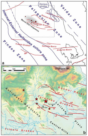
Figure 1.
(a) Simplified geological-tectonic map of Central Greece showing the major isopic zones (blue lines/characters) linking the Internal and External Hellenides relative to the location of the seismic sequence. In red are the Middle-Late Quaternary tectonic structures. The dashed box indicates the enlarged area in (b), in which the major active faults and tectonic structures mapped in the broader epicentral area (modified from [3,6,8]) are represented. Red stars indicate the events with M > 5. DF—Domokos Fault; RF—Rodia Fault; GF—Gyrtoni Fault; TF—Tyrnavos Fault; VS—Vlachogianni segment; LF—Larissa Fault.
The present-day orographic texture of Thessaly and its surroundings is basically oriented NW-SE. This trend is the result of complex polyphase tectonic evolution that began during the Cretaceous period, when the Pelagonian microcontinent [1,2] collided with the Vardar Zone and became attached to the southern margin of Eurasia. On the opposite side, with the progressive subduction of the Pindos Ocean, another branch of Tethys realm, a new collisional process started in the late Eocene or early Oligocene culminating in the creation of the External Hellenides fold-and-thrust belt. The accretionary wedge is still active along the Ionian Sea, but in Thessaly, contractional deformation ended in the (early) Miocene. With the progressive westward migration of thrusting and the consequent local waning of compression, the whole region was then affected (from the late Miocene–Pliocene to the early Pleistocene) by a widespread post-orogenic collapse [3]. This induced a strong tectonic inversion associated with a NE-SW crustal extension and mainly NW-SE trending structures [4]. The overall result was a basin-and-range-like morphology, alternating between tectonic-topographic ‘highs’, like the Pindos Range, the Central Hills and the Olympos-Ossa-Pilion range, and ‘lows’, like the Karditsa, Larissa and Thermaikos basins.
However, since the middle Pleistocene, the geodynamics of the Aegean Region have abruptly changed, with this change being characterized by a roughly longitudinal stretching direction. Thessaly was affected by this most recently, and thus it still has active tectonic phases which have started generating new, mainly E-W trending structures, like the Tyrnavos Graben and Gonnoi Horst [5] or the Almyros and Vasilika Basins [4] in the northern and southern sectors, respectively. Most of the associated normal faults are still in an incipient stage [6], and hence the cumulative displacements are relatively small. Moreover, in several cases, the newly formed seismogenic sources have likely exploited inherited NW-SE trending structures. Clear examples are represented by the Rodia Fault, north of Larissa [7,8], and the Domokos Fault, south of Karditsa [9,10], or the Vlachogianni segment west of Tyrnavos. Whatever the case, the accumulated crustal deformation since the middle–late Quaternary has not yet been sufficient to have radically changed the region-wide morphology of Thessaly.
The seismic sequence that affected northern Thessaly in March 2021 perfectly reflects the above structural and seismotectonic complexities as far as the preliminary available focal mechanisms indicate nodal planes ranging between WNW-ESE and NW-SE. In order to shed some light on the issue, the present research is devoted to analyzing the broader epicentral area by means of the synthetic aperture radar interferometry (InSAR) technique. Indeed, the 2021 Thessaly sequence represents a very uncommon case study where InSAR data allowed us to isolate the coseismic ground deformations due to the major shocks and to provide a first estimate of the geometric and kinematic characteristics of the causative faults. Some other studies have been produced using InSAR methodology to investigate earthquake sequences or swarms worldwide [11,12,13,14,15,16,17,18]. This in turn will contribute to unravel the seismotectonic complexity of the affected crustal volume.
The paper is organized as follows. Section 2 illustrates the InSAR rationale, evidencing its advantages and limitations. In Section 3, we present the results related to both the three different seismic events individually and the cumulated displacement caused by all the events together obtained using the InSAR analysis. In Section 4, we introduce the discussion based on the InSAR outcomes and their interpretation under a morpho-tectonic point of view. Finally, the concluding remarks are addressed in Section 5.
2. InSAR Technique and Data
Over recent decades, InSAR technology [19,20,21] has been used to investigate ground deformations due to seismic, volcanic, geological, or anthropogenic activities. It relies on the extraction of the phase difference between two complex-valued SAR images related to the same imaged scene, usually referred to as master and slave, respectively. An SAR sensor is a coherent, active microwave instrument, which can acquire data during daytime or nighttime, and under virtually all meteorological conditions (i.e., it is time and weather independent). Each SAR image pixel consists of a complex value, obtained as the vector sum (i.e., accounting for amplitude and phase) of the backscattered incident radar pulse from the elementary targets within a resolution cell. The pixel-per-pixel phase difference between two images (the so called interferogram) acquired at different times can be related to the changes in the geometric distance of the radar from the illuminated object, if the backscattered signals are sufficiently correlated. The interferogram contains both topographic and surface motion information; surface motion can be obtained by removing the topographic component in general by using an external DEM (e.g., [20]). Each fringe (i.e., 2π phase difference) corresponds to a line of sight (LoS) displacement equal to λ/2, where λ is the SAR wavelength. Several issues, however, may complicate the application of InSAR to a single image pair.
Firstly, several sources (e.g., vegetation growth, ground movement, soil erosion, plowing, and differences in imaging geometry) may cause the SAR phases at the two acquisitions to be statistically decorrelated [22], and thus unrelated to the changes in the geometric distance from the radar. Secondly, phase differences are only observed in modulus 2π. The recovery of the integer multiples of 2π, and thus the determination of the phase gradient between any two interferogram pixels, represents a 2D phase unwrapping problem, for which only approximate solutions can be found by automated algorithms [23]. Recent coseismic literature ad-hoc phase unwrapping strategies include: manually preventing error-prone integration paths, e.g., across fault ruptures [24] or high fringe-rate areas [25], and manual phase-jump corrections between the mainland and islands [26]. Moreover, if the ground motion results along the North-South direction, the interferometry is not able to detect it (or it is able to only for a fraction of about 10%). To avoid such limitations, some different SAR techniques have been developed such as offset-tracking and multiple aperture interferometry methods [27,28,29,30].
Finally, the measured differences in travel-times (or distances) can also be influenced by unmodeled effects, e.g., due to variable propagation velocity through the variably refractive atmosphere (mainly due to water vapor content) or to uncertainties in the satellite position at the moment of the acquisitions. It is possible to overcome (or at least limit) the atmospheric delay, and as such the multi-temporal InSAR approach (that is not the object of this paper) has been developed over the last two decades and is nowadays widely used, especially to study the post-seismic phase and monitor a large variety of phenomena affecting the Earth’s surface. With the aim of mitigating the undesired contribution of the atmosphere in the coseismic phase, it is possible to introduce tropospheric delay maps from the date in question that can be provided by many external sources (i.e., GACOS delay maps [31]) into the SAR data processing.
The Tyrnavos seismic sequence has been analyzed by using the InSAR technique with the aim of detecting and assessing the complex coseismic ground deformation patterns resulting from different earthquakes. The unprecedented revisit time of 6 days offered by the synergistic action of Sentinel-1A-B missions, operated by the European Space Agency, allows us to provide a synoptic view of the main events of the sequence, i.e., the ML 6.0 mainshock occurred on the 3 March and the strongest aftershocks (ML 5.9 and ML 5.2) occurred on the 4 and 12 March respectively, hereinafter referred to as events 1, 2, and 3 (Table 1). Indeed, according to the acquisition plan, such events can be isolated and investigated by taking advantage of the combined use of all the available Sentinel-1 SAR images. To such aim, three interferograms from Sentinel-1 ascending data (in the TOPSAR acquisition mode) encompassing the coseismic displacement due to each event have been calculated. In addition, two interferograms encompassing all the three events, thus providing the cumulated displacement field for both the ascending and descending orbits, were produced (Table 2). Furthermore, with the cumulated interferograms along both tracks being available, it was possible to calculate the displacement components along the E-W and vertical direction, respectively.
Table 2.
SAR data used to investigate the seismic swarm.
The interferometric pairs were processed using different software (i.e., SARscape (SARMAP), GAMMA [32], and SNAP (provided by ESA)) to perform the standard two-step interferometry and cross-validate the InSAR measurements. Hence, firstly the acquisitions were imported in the format desired by the specific software, then the later image (slave) was coregistered on the earlier one (master). A multilooking factor was applied to obtain a final ground resolution equal to 30 m. Such an operation is also useful to reduce the speckle noise and then increase the signal to noise ratio. Then, the interferogram was calculated and a filtering operation was applied, adopting the Goldstein filter [33]. Interferometric fringes were then unwrapped with the minimum cost flow algorithm [34] and geocoded to get the line of sight (LoS) displacement map. The InSAR topographic contribution was removed using the shuttle radar topography mission SRTM–1 (resolution ∼30 m) digital elevation model [35].
The choice to process all the coseismic interferograms by means of three different software, allowed us to cross-validate the results.
3. Results
We organize this section as follows: first we show the InSAR results for each of the three individual events, and then for the cumulated case. Here, for the sake of simplicity, we show the results retrieved only through GAMMA but all the coseismic pairs were also processed using both the SARScape and SNAP software (these data are provided in the supplementary material).
3.1. Isolated Events
3.1.1. Coseismic Deformation of the 3 March Event
The mainshock of the sequence, i.e., the ML 6.0 earthquake, occurred on the 3 March at 10:16 (UTC), was investigated considering the ascending SAR pair acquired on the 25 February and the 3 March, respectively. The postseismic image was acquired only a few hours after the event, at about 16:30, thus allowing us to capture the coseismic ground displacement. Although acquired on the same dates, the data along the descending orbit were not able to constrain the ground deformation since the image from the 3 March was acquired a few hours before the event.
The mainshock produced a deformation pattern highlighted by the ascending InSAR analysis (Figure 2A,B). The full deformation pattern occurred in an area located a few kilometers away from the epicenter towards the south-west, and seems to have been caused by a normal fault that was, until now, unknown, elongating NW-SE with a ~20 km length, as is clearly visible from the obtained interferogram. Moreover, the epicenter is in an area very seldom affected by seismic events in recent years (Figure 1). The maximum displacement values reach more than 25 cm away from the satellite along the line of sight (LoS); the obtained full deformation field affects an area of ~20 km in length and ~10 km in width.
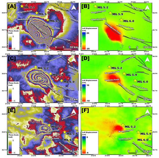
Figure 2.
Wrapped interferogram and LoS displacement related to the ML 6.0 mainshock (A,B); the ML 5.9 aftershock (C,D) and the ML 5.2 aftershock (E,F). The epicenter locations are from the National Observatory of Athens (NOA) (http://www.gein.noa.gr/en/seismicity/recent-earthquakes, accessed on 20 March 2021). The active faults modified from [3,6,8].
3.1.2. Coseismic Deformation of the 4 March Event
The day after the mainshock, a strong aftershock ML 5.9 struck the same area only a few kilometers NW from the main event. We considered the ascending interferometric couple spanning the temporal interval 3–9 March to image the earthquake (Figure 2C,D). The retrieved pattern was comparable with the previous one but obviously moved towards the NW with a lower length (about 12 km) and values (up to ~10 cm). Also, in this case, the causative fault seems to be a new normal fault or a consecutive segment of the previous one. The epicenter of this new event is located NW with respect to the mainshock that showed a SE-NW alignment.
3.1.3. Coseismic Deformation of the 12 March Event
A number of aftershocks occurred, so on 12 March, a new earthquake ML 5.2 affected the area 20 km NW to the 4 March event. The ground movement was imaged using the Sentinel-1 data acquired along the ascending orbit (Figure 2E,F). Looking at the obtained pattern, we got maximum LoS values of ~−6 cm, and a length of less than 10 km. Furthermore, looking at this final moderate event, the NW-SE alignment is confirmed concerning both the three event epicenters and the produced surface displacement fields.
3.2. Cumulated Events
Once we isolated the three earthquakes, we produced the cumulated displacement pattern due to all events combined. To this end, we selected two interferometric pairs along both the ascending and descending orbit. In detail, we considered the 25 February 2021 and the 15 March 2021 data for the ascending direction and the 2 March 2021 and the 14 March 2021 acquisitions for the descending one. The ascending and descending retrieved displacement patterns take into account both the coseismic deformations induced by the 3 main events as well as any postseismic release. However, the interferograms obtained from InSAR show several fringes quite well recognized and associated with significant deformation signals. Deformation is due to the 3 different events and is aligned along the SE-NW direction with a total length of about 45 km and a maximum width of more than 15 km. The phase interferograms were unwrapped and the LoS deformation motions were estimated, revealing strong co-seismic displacements mainly in the Northern and Western part of the Tyrnavos area.
The ascending cumulated interferogram (Figure 3A,C) shows a similar shape and number of deformational fringes to the ones formed in the descending pair (Figure 3B,D). The latter is indicative of the preeminent vertical kinematic character of the ground movement depicted from the two SAR geometries along the LoS directions.
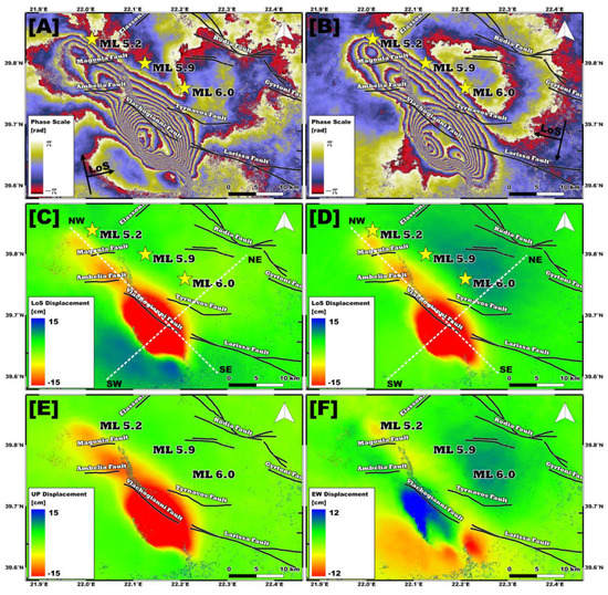
Figure 3.
Wrapped ascending and descending interferograms (A,B), LoS displacement (C,D), and UP (E) and EW (F) deformation component srelated to the cumulated coseismic ground deformation of the ML 6.0, ML 5.9, and ML 5.2 earthquakes. The dashed lines in panels (C,D) indicate the cross sections shown in Figure 4.
The LoS displacement vector is composed by the displacement along the E-W, N-S, and vertical components projected along the SAR sensor direction. Based on the satellite SAR acquisition geometry, the projection of the LoS displacement vector on the 3D motion components is defined by the incidence angle θ and the azimuth angle φ of the satellite heading (measured clockwise from the North). Moreover, due to the characteristic imaging mode, the InSAR technique is more sensitive in revealing the vertical motions than the E-W motions, while it is limited in the N-S direction. Taking advantage of the availability of both the ascending and descending SAR geometry for the common ground pixel, we combined LoS cumulated displacement measurements to estimate the horizontal and vertical components of the total detected displacement signal (Figure 3E,F). During this calculation, both the azimuth and incidence angles of the satellite were treated as constants for each track [36]. The E-W component deformation map (Figure 3F) depicts significant eastward motion of the interested area (~10 cm), while the vertical component describes strong subsidence phenomena up to more than 10 cm (Figure 3E). The images of the E-W and vertical components emphasize the gradual decrease in co-seismic displacement towards the Western and Northern part of the Tyrnavos area.
Then, to better analyze the retrieved deformation patterns, we performed two parallel profiles along the two sections shown in Figure 3C,D, crossing the cumulated LoS displacement field SE-NW and SE-NW in the NE-SW direction, and across the cumulated LoS displacement fields (Figure 4A,B). It is noteworthy as the reliability of the measurements is guaranteed by the cross-validation of the outcomes from different software shown in all panels. InSAR measurements from SNAP, SARScape, and GAMMA are in excellent agreement, showing the same behavior along both transects. The deformation patterns due to the three events projected along the SE-NW cross sections (Figure 4A,C) are well recognized, especially thanks to the descending data. Here, starting from SE to NW, it is possible to detect three minima of the deformation pattern in correspondence with the epicenters of the events peaking at about −30, −10, and −6 cm, respectively. Concerning the NE-SW sections, +10 cm of LoS deformation are measured along the two sides of the main pattern in ascending (Figure 4C) and descending (Figure 4D) data. It is consistent with the estimated EW deformation (Figure 3F).
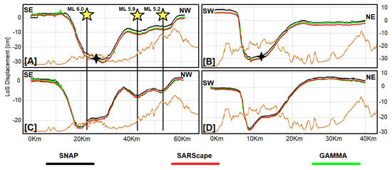
Figure 4.
Cross sections along the SE-NW and SW-NE transects shown in Figure 3 panels (C,D) for the cumulated ascending (A,B) and descending (C,D) LoS displacement maps. Blue cross indicates the crossing point between the two profiles.
Looking at Figure 4, it is easy to see how the displacement values retrieved from the cumulated coseismic pairs obtained from the different software are essentially equivalent to each other. Furthermore, the SE-NW transects initially exhibit the larger ground displacement pattern due to the mainshock then a resurgence (motion towards the sensor) of the surface movement and two new consecutive soil displacements (motion away from the sensor) related to the two aftershocks considered in the analysis. Such behavior is common to both the cumulative displacement pattern retrieved from the ascending and descending orbit. In detail, along the descending track, the maximum negative value is about −30 cm due to the larger magnitude earthquake while the following two events reach −12 cm and −8 cm, respectively. The ascending cumulative displacement field highlights slightly lower values than the descending case, at up to −20 cm for the mainshock and −8 cm and −6 cm for the aftershocks. The latter probably is due to the different acquisition geometries as well as than a possible small residual related to the atmospheric contribution that does not invalidate the results.
Instead, concerning the SW-NE profile, the retrieved patterns for both orbits show as their main behavior a fast increase in the sensor-target distance (negative values) occurring at a very short distance of less than ~3 km with values up to ~30 cm (~28 for the ascending case) followed by a rise for a total length of ~15 km.
These patterns suggest that they are due to the presence of one or more normal faults showing a roughly NW-SE strike and a common NE dipping with a length of more than 40 km.
4. Discussion
The interferometric analyses suggest that the activation of a NW-SE trending, ~20 km long normal fault for the 3 March 2021 ML 6.0 mainshock. Based on a joint analysis with preliminary seismological data and field observations [37], the causative fault is deemed to be NE-dipping at a relatively moderate angle (~35°). Both interferometric results (see the transects in Figure 4) and the first available focal mechanisms (NOA, INGV, USGS, GFZ, EMSC) support this hypothesis, which leads us to some inferences about the role played by the local geological setting for the seismic sequence nucleation and faulting propagation.
For this purpose, and in order to provide additional seismotectonic constraints to the sequence characterization, we realized several rheological profiles in the epicentral area(s) of the mainshocks. A comparison and cross-check between the modelled rheological layering and the preliminary seismological data, with particular reference to the depth distribution of the seismicity, has been carried out. Such an approach follows a long-established concept in the earthquake geology literature (e.g., [38,39]), linking the seismological behavior to the brittle deformation. Accordingly, the brittle-ductile transition (hereinafter BDT) is generally considered a good approximation for the seismicity cutoff depth.
The strength envelopes have been realized after a thorough selection of the input parameters for the modelling of the brittle and ductile behaviors (respectively corresponding to frictional sliding and power-law creep deformation mechanisms), following the methods and the indications provided in Maggini and Caputo [40,41]. Specific and accurate elaborations on the most crucial parameters (see [41]), such as the thermal ones, surface heat flow, crustal structure, Moho depth, and strain rate have been carried out starting from the available literature data (e.g., [42,43,44]). The resulting rheological profiles for the epicentral area indicate that the BDT lies at ca 17–18 km (Figure 5).
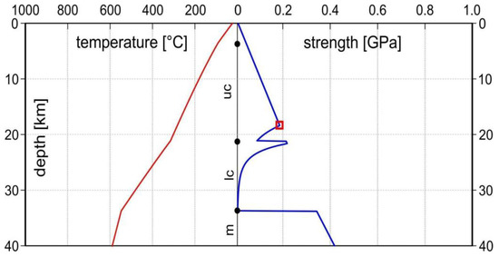
Figure 5.
Representative rheological profile for the epicentral area. The blue line represents the strength envelope, the red line the corresponding geothermal gradient, while the red square indicates the BDT. Abbreviations: uc—upper crust; lc—lower crust; m—mantle.
Most of the aftershocks in the sequence are confined in the first 15 km of the crust [37], with the mainshocks being limited to maximum depths of ~10 km. On one hand, such seismological features agree with the proposed rheological layering, as the seismicity is effectively limited to (the upper portion of) the brittle layer. On the other hand, however, the slight discrepancy between the deeper BDT and the shallower seismicity cutoff depth of the March 2021 sequence may be pointing out that seismicity nucleation and faulting propagation are, here, also controlled by the litho-mechanical setting and geological evolution rather than by the very rheological layering itself.
To this point, it is worth noting that the crustal(-lithospheric) suture between the Internal and the External Hellenides recalled in the introduction (Figure 1a), that is to say the major shear zone separating the overthrusted Pelagonian units from the underlying Pindos Ocean, including interposed slices of the ophiolithic suite, largely outcrops along the western sectors of Thessaly, but also within the Olympus, Ossa and Krania tectonic windows. Taking into account reasonable thickness values of the Pelagonian and the other involved tectono-stratigraphic units, in correspondence with the epicentral area of the March 2021 seismic sequence, this important weakness zone is relatively shallow, say between 5 and 10 km deep, and it is likely affected by major vertical steps reasonably caused by the high angle Neogene-Quaternary faulting. We therefore suggest that the causative fault for the March 2021 sequence may be tentatively linked to some of these inherited structures in the relatively shallow and weak volume, corresponding to the suture zone between Internal and External Hellenides. With this in mind, it should also be noted that such faults and shear zones may have possibly acted earlier as compressional structures and then been subjected to negative inversion. Accordingly, they may still retain peculiar features of compressional tectonics, such as the low-to-moderate dip angle, which may represent a potential explanation for the small/moderate dip seen in the available focal mechanisms for the March 2021 sequence.
5. Concluding Remarks
The present ground deformation study based on InSAR analysis and geological interpretation of the Thessaly seismic swarm outlines the seismogenic source and provides an overall image of the tectonic status in the investigated area. InSAR data exhibit intense displacements on the southern and eastern part of the affected area, decaying towards its western and northern parts. The pattern and amplitude of the InSAR LoS displacement vectors, and the decomposed E-W and vertical components, highlighted distinct and differential motions along and across the different tectonic structures. Co-seismic displacements during the occurred sequence are correlated with the activation of a SE-NW striking normal fault system largely unknown in its details, but clearly belonging to the Tyrnavos Graben that started forming in the middle-late Pleistocene, and whose bordering structures are still in a growing phase.
Accordingly, all investigated events could certainly be considered ‘areal’ morphogenic earthquakes, but not ‘linear’ ones [45].
An improvement/extension of this work could be to consider other SAR data acquired at different frequency bands such as L- and X-Band and line of sight. In this way, it would be possible to retrieve the whole 3-D deformation coseismic field. Furthermore, it could be interesting to follow this study producing the source model for the causative faults.
It is noteworthy to highlight the capacity to discriminate between each of the three different events providing a fairly unique possibility to underline the various retrieved patterns and the related ground displacement values evidencing the SE-NW alignment. Isolating, through InSAR data, the contribution of each event in a seismic sequence occurring in a short time span is not straightforward. This is due to the revisit time of the satellite and the high temporal frequency of the seismic events in a sequence. The previous C-band mission of the European Space Agency (ESA), i.e., ERS and Envisat, were able to acquire one SAR image per month. Therefore, they are constrained to the cumulated ground displacement related to a seismic sequence occurring for 7–10 days, as did the Thessaly sequence.
Instead, the launch of Sentinel-1 missions opened new scenarios and possibilities in the study of seismic sequences. They offer an unprecedented revisit time of 6 days thanks to the synergistic action of both Sentinel-1A and Sentinel-1B satellites. Such revisit time is an essential condition in order to separate the contribution of any foreshocks and/or aftershocks from the mainshock. However, it may not be sufficient. Indeed, as in this investigated case, it is important to have a suitable correlation between the Sentinel-1 acquisition plan and the occurrence of the seismic events so that to have at least one SAR acquisition before and after any significant earthquake of the sequence. Finally, InSAR analysis has proved to be a fundamental instrument for monitoring interesting phenomena on the Earth’s surface, such is a seismic swarms, in a unique way that helps support geophysics and decision makers as well. We demonstrate here that the Sentinel-1 constellation could potentially provide unprecedented opportunities to study these phenomena, and even face the low temporal resolution of InSAR.
Supplementary Materials
The following are available online at https://www.mdpi.com/article/10.3390/geosciences11050191/s1. All the analyzed coseismic pairs used in this work are enclosed in a rar file. Such file shows a DOI assigned through the Zenodo site: 10.5281/zenodo.4659820.
Author Contributions
R.C., S.S., and C.T. conceived the project; C.T., M.P., and N.A.F. analyzed the SAR data; R.C. and M.M. provided the geological knowledge of the area of Tyrnavos and deeply helped with the interpretation of the experimental results; all authors contributed to the writing. All authors have read and agreed to the published version of the manuscript.
Funding
This research received no external funding.
Institutional Review Board Statement
Not Applicable.
Informed Consent Statement
Not Applicable.
Data Availability Statement
The data presented in this study are openly available in Zenodo at https://zenodo.org/record/4659820#, accessed on 28 April 2021. YIpghZAzZdg [doi:10.5281/zenodo.4659820].
Acknowledgments
The authors thank the European Space Agency (ESA) for distributing the Sentinel-1 SAR images of the Tyrnavos area, which were used in this work, free of charge.
Conflicts of Interest
The authors declare no conflict of interest.
References
- Mountrakis, D. Tertiary and Quaternary tectonics of Greece. In Postcollisional Tectonics and Magmatism in the Mediterranean Region and Asia; Dilek, Y., Pavlides, S., Eds.; Geological Society of America: Boulder, CO, USA, 2006; Volume 409, pp. 125–136. [Google Scholar]
- Doutsos, T.; Pe-Piper, G.; Boronkay, K.T.; Koukouvelas, I. Kinematics of the central Hellenides. Tectonics 1993, 12, 936–953. [Google Scholar] [CrossRef]
- Caputo, R.; Pavlides, S. Late Cainozoic geodynamic evolution of Thessaly and surroundings (central-northern Greece). Tectonophys 1993, 223, 339–362. [Google Scholar] [CrossRef]
- Caputo, R. Geological and structural study of the recent and active brittle deformation of the Neogene-Quaternary basins of Thessaly (Greece). Sci. Ann. 1990, 2, 252. [Google Scholar]
- Caputo, R.; Bravard, J.-P.; Helly, B. The Pliocene-Quaternary tecto-sedimentary evolution of the Larissa Plain (Eastern Thessaly, Greece). Geodin. Acta 1994, 7, 57–85. [Google Scholar] [CrossRef]
- Caputo, R. Inference of a seismic gap from geological data: Thessaly (Central Greece) as a case study. Ann. Geofis. 1995, 38, 1–19. [Google Scholar]
- Caputo, R. Morphotectonics and kinematics along the Tirnavos Fault, northern Larissa Plain, mainland Greece. Zeits. Geomorph. NF 1993, 94, 167–185. [Google Scholar]
- Caputo, R.; Helly, B. The Holocene activity of the Rodia Fault, Central Greece. J. Geodyn. 2005, 40, 153–169. [Google Scholar] [CrossRef]
- Papastamatiou, D.; Mouyaris, N. The earthquake of April 30, 1954, in Sophades (Central Greece). Geophys. J. R. Astron. Soc. 1986, 87, 885–895. [Google Scholar] [CrossRef]
- Palyvos, N.; Pavlopoulos, K.; Froussou, E.; Kranis, H.; Pustovoytov, K.; Forman, S.L.; Minos-Minopoulos, D. Paleoseismological investigation of the oblique-normal Ekkara ground rupture zone accompanying the M 6.7–7.0 earthquake on 30 April 1954 in Thessaly, Greece: Archaeological and geochronological constraints on ground rupture recurrence. J. Geophys. Res. 2010, 115, B06301. [Google Scholar]
- Svigkas, N.; Atzori, S.; Kiratzi, A.; Tolomei, C.; Salvi, S. Isolation of swarm sources using InSAR: The case of the February 2017 seismic swarm in western Anatolia (Turkey). Geophys. J. Int. 2019, 217, 1479–1495. [Google Scholar] [CrossRef]
- Pezzo, G.; Tolomei, C.; Atzori, S.; Salvi, S.; Shabanian, E.; Bellier, O.; Farbod, Y. New kinematic constraints of the western Doruneh Fault, northeastern Iran, from interseismic deformation analysis. Geophys. J. Int. 2012, 190, 622–628. [Google Scholar] [CrossRef]
- Salvi, S.; Atzori, S.; Tolomei, C.; Antonioli, A.; Trasatti, E.; Merryman Boncori, J.P.; Pezzo, G.; Coletta, A.; Zoffoli, S. Results from INSAR monitoring of the 2010–2011 New Zealand seismic sequence: EA detection and earthquake triggering. In Proceedings of the IEEE International Symposium on Geoscience and Remote Sensing (IGARSS), Munich, Germany, 22–27 July 2012; pp. 3544–3547. [Google Scholar]
- Atzori, S.; Tolomei, C.; Antonioli, A.; Merryman Boncori, J.P.; Bannister, S.; Trasatti, E.; Pasquali, P.; Salvi, S. The 2010–2011 Canterbury, New Zealand, seismic sequence: Multiple source analysis from InSAR data and modeling. J. Geophys. Res. 2012, 117, B08305. [Google Scholar] [CrossRef]
- Bell, J.; Amelung, F.; Christopher, H. InSAR analysis of the 2008 Reno-Mogul earthquake swarm: Evidence for westward migration of Walker Lane style dextral faulting. Geophys. Res. Lett. 2012, 39, L18306. [Google Scholar] [CrossRef]
- Benetatos, C.; Kiratzi, A.; Kementzetzidou, K.; Roumelioti, Z.; Karakaisis, G.; Scordilis, E.; Latoussakis, I.; Drakatos, G. The Psachna (Evia Island) earthquake swarm of June 2003. Bull. Geol. Soc. Greece 2004, 36, 1379–1388. [Google Scholar] [CrossRef]
- Kyriakopoulos, C.; Chini, M.; Bignami, C.; Stramondo, S.; Ganas, A.; Kolligri, M.; Moshou, A. Monthly migration of a tectonic seismic swarm detected by DInSAR: Southwest Peloponnese, Greece. Geophys. J. Int. 2013, 194, 1302–1309. [Google Scholar] [CrossRef]
- Ganas, A.; Kourkouli, P.; Briole, P.; Moshou, A.; Elias, P.; Parcharidis, I. Coseismic displacements from moderate-size earthquakes mapped by Sentinel-1 differential interferometry: The case of February 2017 Gulpinar earthquake sequence (Biga Peninsula, Turkey). Remote Sens. 2018, 10, 1089. [Google Scholar] [CrossRef]
- Gabriel, A.K.; Goldstein, R.M.; Zebker, H.A. Mapping small elevation changes over large areas: Differential radar interferometry. J. Geophys. Res. Solid Earth 1989, 94, 9183–9191. [Google Scholar] [CrossRef]
- Massonnet, D.; Rossi, M.; Carmona, C.; Adragna, F.; Peltzer, G.; Feigl, K.; Rabaute, T. The displacement field of the Landers earthquake mapped by radar interferometry. Nature 1993, 364, 138–142. [Google Scholar] [CrossRef]
- Peltzer, G.; Rosen, P. Surface Displacement of the 17 May 1993 Eureka Valley, California, Earthquake Observed by SAR Interferometry. Science 1995, 268, 1333–1336. [Google Scholar] [CrossRef]
- Zebker, H.A.; Villasenor, J. Decorrelation in interferometric radar echoes. IEEE Trans. Geosci. Remote Sens. 1992, 30, 950–959. [Google Scholar] [CrossRef]
- Chen, C.W.; Zebker, H.A. Two-dimensional phase unwrapping with use of statistical models for cost functions in nonlinear optimization. J. Opt. Soc. Am. 2001, 18, 338–351. [Google Scholar] [CrossRef]
- Yue, H.; Simons, M.; Duputel, Z.; Jiang, J.; Fielding, E.; Liang, C.; Owen, S.; Moore, A.; Riel, B.; Ampuero, J.P.; et al. Depth varying rupture properties during the 2015 Mw 7.8 Gorkha (Nepal) earthquake. Tectonophysics 2017, 714–715, 44–54. [Google Scholar] [CrossRef]
- Wang, T.; Wei, S.; Shi, X.; Qiu, Q.; Li, L.; Peng, D.; Weldon, R.J.; Barbot, S. The 2016 Kaikoura earthquake: Simultaneous rupture of the subduction interface and overlying faults. Earth Planet. Sci. Lett. 2018, 482, 44–51. [Google Scholar] [CrossRef]
- Moreno, M.; Li, S.; Melnick, D.; Bedford, J.R.; Baez, J.C.; Motagh, M.; Metzger, S.; Vajedian, S.; Sippl, C.; Gutknecht, B.D.; et al. Chilean megathrust earthquake recurrence linked to frictional contrast at depth. Nat. Geosci. 2018, 11, 285–290. [Google Scholar] [CrossRef]
- Mastro, P.; Serio, C.; Masiello, G.; Pepe, A. The Multiple Aperture SAR Interferometry (MAI) Technique for the Detection of Large Ground Displacement Dynamics: An Overview. Remote Sens. 2020, 12, 1189. [Google Scholar] [CrossRef]
- Bechor, N.B.D.; Zebker, H.A. Measuring two-dimensional movements using a single InSAR pair. Geophys. Res. Lett. 2006, 33, L16311. [Google Scholar] [CrossRef]
- Avouac Michel, R.; Taboury, J.P. Measuring ground displacements from SAR amplitude images: Application to the Landers earthquake. Geophys. Res. Lett. 1999, 26, 875–878. [Google Scholar] [CrossRef]
- Peltzer, G.; Crampé, F.; King, G. Evidence of nonlinear elasticity of the crust from the Mw 7.6 Manyi (Tibet) earthquake. Science 1999, 286, 272–276. [Google Scholar] [CrossRef]
- Li, X.; Huang, G.; Kong, Q. Atmospheric phase delay correction of D-InSAR based on Sentinel-1A. Int. Arch. Photogramm. Remote Sens. Spat. Inf. Sci. 2018, XLII-3, 955–960. [Google Scholar] [CrossRef]
- Wegmuller, U.; Werner, C. Gamma SAR processor and interferometry software. In Proceedings of the ERS Symposium on Space at the Service of Our Environment; ESA Publications Division: Florence, Italy, 1997; pp. 1687–1692. [Google Scholar]
- Goldstein, R.M.; Werner, C.L. Radar interferogram filtering for geophysical applications. Geophys. Res. Lett. 1998, 25, 4035–4038. [Google Scholar] [CrossRef]
- Costantini, M. A novel phase unwrapping method based on network programming. IEEE Trans. Geosci. Remote Sens. 1998, 36, 813–821. [Google Scholar] [CrossRef]
- Farr, T.G.; Kobrick, M. Shuttle radar topography mission produces a wealth of data. Eos Trans. AGU 2000, 81, 583–585. [Google Scholar] [CrossRef]
- Dalla Via, G.; Crosetto, M.; Crippa, B. Resolving vertical and east-west horizontal motion from differential interferometric synthetic aperture radar: The L’Aquila earthquake. J. Geophys. Res. 2012, 117, B02310. [Google Scholar] [CrossRef]
- Lekkas, E.; Agorastos, K.; Mavroulis, S.; Kranis, C.; Skourtsos, E.; Carydis, P.; Gogou, M.; Katsetsiadou, K.-N.; Papadopoulos, G. The early March 2021 Thessaly earthquake sequence. Newsl. Environ. Disaster Cris. Manag. Strateg. 2021, 195. [Google Scholar] [CrossRef]
- Scholz, C.H. The brittle-plastic transition and the depth of seismic faulting. Geol. Rundsch. 1988, 77, 319–328. [Google Scholar] [CrossRef]
- Sibson, R.H. Roughness at the Base of the Seismogenic Zone: Contributing Factors. J. Geophys. Res. 1984, 89, 5791–5799. [Google Scholar] [CrossRef]
- Maggini, M.; Caputo, R. Rheological behaviour in collisional and subducting settings: Inferences for the seismotectonics of the Hellenic Region. Turk. J. Earth Sci. 2020, 29, 381–405. [Google Scholar]
- Maggini, M.; Caputo, R. Sensitivity analysis for crustal rheological profiles: Examples from the Aegean Region. Ann. Geophys. 2020, 63, SE334. [Google Scholar] [CrossRef]
- Makris, J.; Papoulia, J.; Yegorova, T. A 3-D density model of Greece constrained by gravity and seismic data. Geophys. J. Int. 2013, 194, 1–17. [Google Scholar] [CrossRef]
- Fytikas, M.D.; Kolios, N.P. Preliminary heat flow map of Greece. In Terrestrial Heat Flow in Europe; Springer: Berlin/Heidelberg, Germany, 1979; pp. 197–205. [Google Scholar]
- Kreemer, C.; Blewitt, G.; Klein, E.C. A geodetic plate motion and Global Strain Rate Model. Geochem. Geophys. 2014, 15, 3849–3889. [Google Scholar] [CrossRef]
- Caputo, R. Ground effects of large morphogenic earthquakes. J. Geodyn. 2005, 40, 113–118. [Google Scholar] [CrossRef]


Publisher’s Note: MDPI stays neutral with regard to jurisdictional claims in published maps and institutional affiliations. |
© 2021 by the authors. Licensee MDPI, Basel, Switzerland. This article is an open access article distributed under the terms and conditions of the Creative Commons Attribution (CC BY) license (https://creativecommons.org/licenses/by/4.0/).