Instability of Compacted Residual Soil

Abstract

Static liquefaction of loose sands has been observed to initiate at stress ratios far less than the steady-state stress ratio. Different collapse surface concepts largely based on undrained triaxial test results have been proposed in the literature to explain the above instability phenomenon of loose sands. Studies of the instability behavior of fill material derived from residual soils remain limited. The present study investigated the instability behavior of a compacted residual soil using the conventional undrained triaxial tests and specially equipped constant shear triaxial tests. The test results were characterized in the p’: q: v space using the current state parameter with respect to the steady-state line for the residual soil. A modified collapse surface that has gradients varying with p’ and v was proposed for the loose residual soil to represent the instability states of undrained loading. Under constant shear stress conditions, the soil can mobilize stress ratios higher than those defined by the modified collapse surface. An instability surface was therefore presented for the instability states reached in static loading. Further, an alternative method of deducing the instability surface from the undrained stress paths was introduced.

1. Introduction

Liquefaction of loose saturated materials has been observed to initiate at a mobilized stress ratio well below the steady-state stress ratio [1,2,3,4]. Sladen et al. [1] introduced the concept of the collapse surface in p’: q: v space based on the peak states of undrained stress paths for the loose sand to explain the instability phenomenon. Sasitharan et al. [5] proposed that the envelope composed of post-peak portions of the undrained stress paths for loose samples defines the state boundary in p’: q: v space (above which no stress state can exist for the soil). Sasitharan et al. [6] approximated the state boundary by a planar envelope passing through the steady-state line. They showed that liquefaction could be initiated when the stress paths for loose materials approach the state boundary surface in either drained or undrained loading.

The above collapse concepts of static liquefaction are largely based on the results of conventional undrained triaxial tests on loose sands. Most of the liquefaction failures in slopes are induced by the reduction in effective confining stress whilst shear stress remains nearly constant, as opposed to the failures reproduced by increasing shear stress in conventional triaxial tests. This difference was first noted by Bishop and Henkel [7]. Brand [8] emphasized that laboratory studies be focused on constant shear stress tests to closely simulate the field stress path.

This study investigated the instability of a compacted residual soil using isotropically consolidated undrained (ICU) and specially equipped constant shear (CS) triaxial tests on specimens of various densities. The parameters associated with the collapse surface concepts and steady states of the soil were obtained from the ICU tests. The CS tests were used to characterize the instability states in static loading and to examine the applicability of the existing collapse surface concepts for the compacted residual soil.

2. Experimental Program

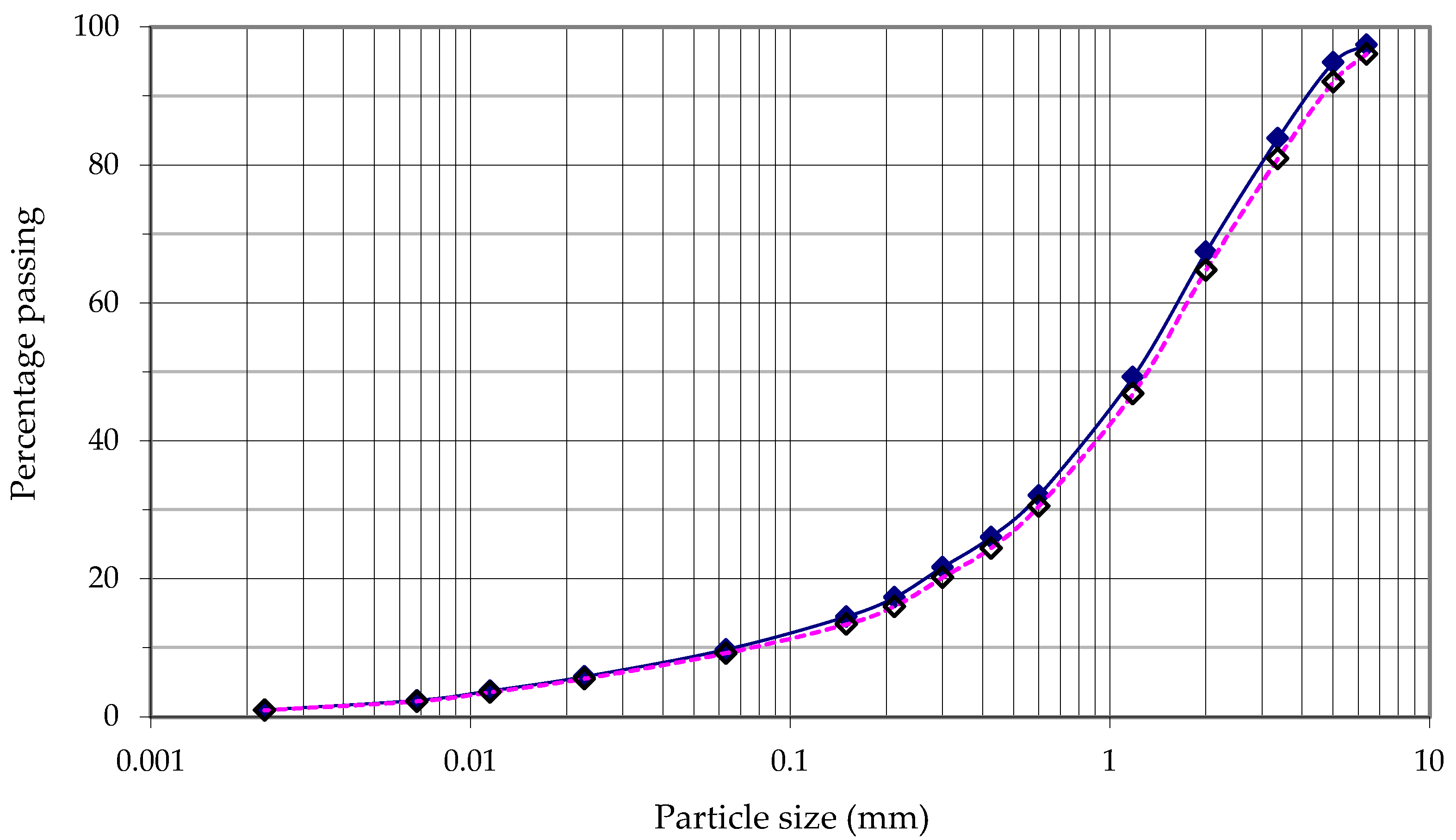
A bulk sample of completely decomposed granite was taken from Beacon Hill in Hong Kong. Based on visual inspection, it was a sandy residual soil and yellowish-brown in color. The particle size distribution of the soil is shown in Figure 1 and the index properties of the soil are summarized in Table 1. According to the British classification system, the soil can be classified as well-graded, silty, gravelly sand. The results of the standard Proctor test indicated a maximum dry density (γ_d(max)) of 1900 kg/m³ and an optimum moisture content of 12.5%.

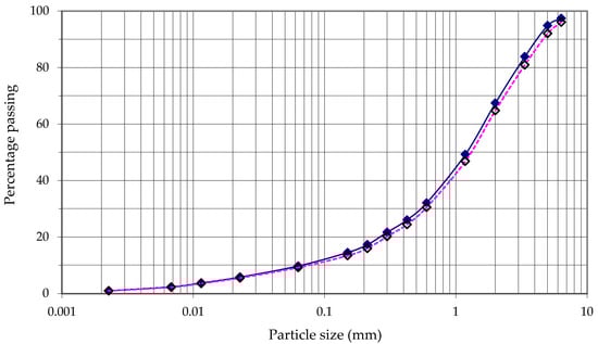
Figure 1. Particle size distribution of the residual soil.

Table 1. Index properties of the residual soil.

Property	Value
Gravel	35%
Sand	55%
Silt	8%
Clay	2%
D10	0.07 mm
D30	0.55 mm
D60	1.65 mm
Liquid limit 1	45%
Plastic limit 1	30%
Specific gravity	2.62

¹ For the material passing 425 μm BS sieve.

Four series of ICU tests were conducted on specimens prepared at void ratios corresponding to target relative compactions Rc (${\gamma }_d$/${\gamma }_{d(\max )}$) ranging from 80% to 95%. The details of the test series are presented in Table 2. For the CS tests, the target relative compactions (Rc) ranged from 80% to 90%. The CS specimens were consolidated to two ranges of principal stress ratios, ${\sigma }_1^{\text{'}}$/${\sigma }_3^{\text{'}}$. The lower stress range ${\sigma }_1^{\text{'}}$/${\sigma }_3^{\text{'}}$ varied from 1.6 to 1.8 and the upper range ${\sigma }_1^{\text{'}}$/${\sigma }_3^{\text{'}}$ was between 2.1 and 2.9. Table 3 summarizes the details of the CS test program.

Table 2. Isotropically consolidated undrained (ICU) test series.

Test Series	Test	Rc (%)	γd (Mg/m3)	After Consolidation		Peak State		Steady State
				p’c	ec	p’p	qp	p’ss	qss
ICU-80	ICU-80-1	80	1.52	34	0.696	24	26	3	5
	ICU-80-2	80	1.52	71	0.660	42	46	11	14
	ICU-80-3	80	1.52	85	0.640	60	60	16	22
	ICU-80-4	80	1.52	102	0.640	71	68	17	25
	ICU-80-5	80	1.52	129	0.624	85	84	23	34
ICU-85	ICU-85-2	85	1.62	42	0.622	43	57	17	27
	ICU-85-3	85	1.62	68	0.605	58	73	22	35
	ICU-85-4	85	1.62	99	0.592	71	77	30	47
	ICU-85-5	85	1.62	122	0.585	83	89	38	58
	ICU-85-6	85	1.62	172	0.559	108	121	52	76
	ICU-85-7	85	1.62	196	0.551	118	137	60	90
ICU-90	ICU-90-1	90	1.71	42	0.527	71	110	-	-
	ICU-90-2	90	1.71	69	0.527	91	135	-	-
	ICU-90-3	90	1.71	98	0.524	111	161	68	106
	ICU-90-4	90	1.71	125	0.519	129	177	75	113
ICU-95	ICU-95-1	95	1.81	40	0.454	171	269	-	-
	ICU-95-2	95	1.81	67	0.448	206	317	-	-
	ICU-95-3	95	1.81	94	0.442	211	326	-	-
	ICU-95-4	95	1.81	122	0.441	239	370	-	-

Notes: Specimens were prepared at the optimum moisture content of 12.5%, Rc: target relative compaction, γ_d: dry density of the specimen at the end of compaction, strain rate: 0.08 mm /min.

Table 3. Constant shear (CS) test series.

Test Series	Test	Rc (%)	γd (Mg/m3)	Isotropic Consolidation		Anisotropic Consolidation
				p’c	ec	p’ac	(q/p’)ac	eac
CS-80	CS-80-1	80	1.52	45	0.672	58	0.57	0.653
	CS-80-2	80	1.52	68	0.671	87	0.57	0.643
	CS-80-3	80	1.52	69	0.679	88	0.57	0.655
	CS-80-4	80	1.52	97	0.655	126	0.52	0.641
CS-85	CS-85-1	85	1.62	94	0.586	118	0.59	0.572
	CS-85-1R	85	1.62	96	0.596	118	0.61	0.582
	CS-85-2	85	1.62	73	0.600	91	0.58	0.596
	CS-85-3	85	1.62	97	0.617	118	0.57	0.611
	CS-85-4	85	1.62	120	0.585	148	0.58	0.578
CS-85B	CS-85B-3	85	1.62	39	0.609	54	0.83	0.606
	CS-85B-4	85	1.62	47	0.613	68	0.88	0.609
	CS-85B-5	85	1.62	64	0.607	89	0.88	0.595
CS-90	CS-90-1	90	1.71	42	0.527	52	0.56	0.525
	CS-90-2	90	1.71	67	0.521	84	0.54	0.519
	CS-90-3	90	1.71	99	0.511	128	0.55	0.507
	CS-90B-1	90	1.71	33	0.523	53	1.15	0.522
	CS-90B-2	90	1.71	28	0.533	42	1.05	0.532
	CS-90B-3	90	1.71	18	0.533	28	1.09	0.533

Notes: Specimens were prepared at the optimum moisture content of 12.5%, Rc: target relative compaction, γ_d: dry density of the specimen at the end of compaction.

2.1. Testing Arrangement

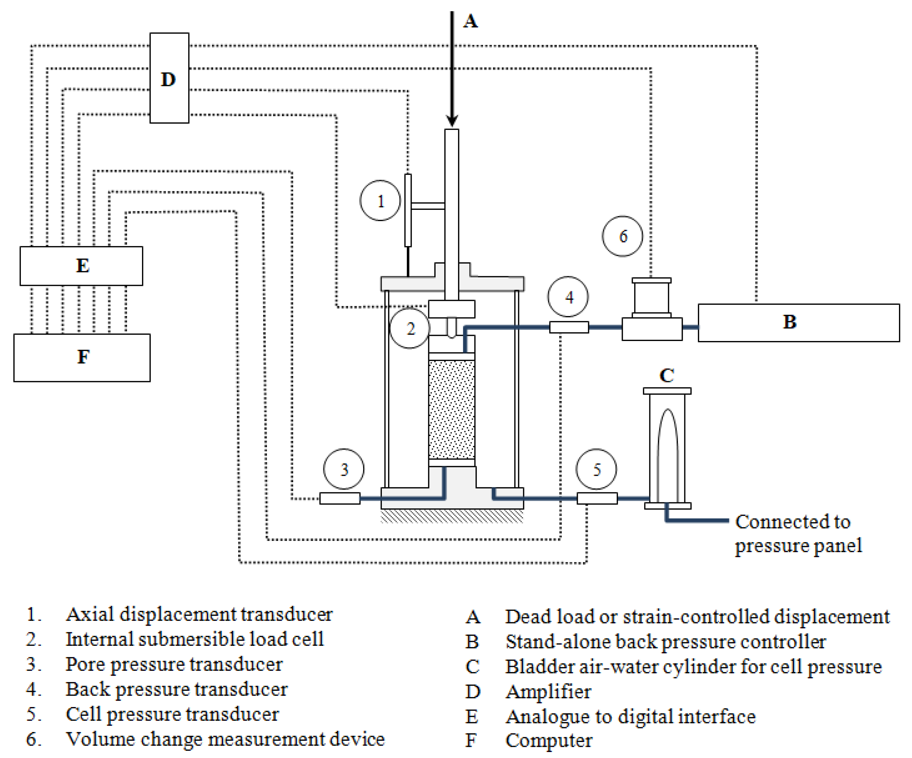
Constant shear triaxial tests can be performed either by reducing the cell pressure while maintaining the back pressure and deviator stress or by increasing the back pressure while maintaining the cell pressure and deviator stress. The second method was used in this study. The triaxial setup consisted of a triaxial cell, a bladder air–water pressure cylinder, a stand-alone back pressure controller, a hanger straddling over the triaxial cell, a load frame, and a high-speed data acquisition system (Figure 2). The hanger with dead weight was used for the CS tests and the load frame was used to apply strain-controlled displacement for ICU tests. The data acquisition system consisted of three pressure transducers, an internal submersible load cell, a volume change measurement device, an axial displacement transducer, an amplifier, and a computer with an analog-to-digital card.

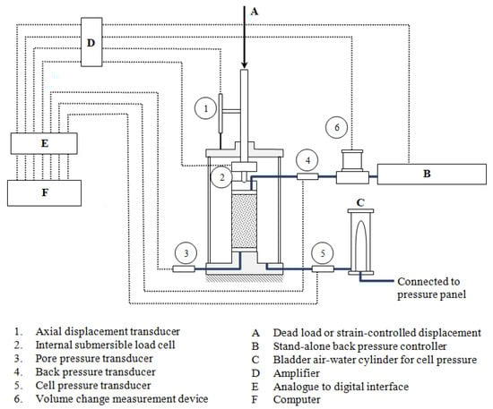
Figure 2. Test arrangements.

The back pressure was controlled by the stand-alone back pressure controller. The cell pressure was maintained constant by the bladder air–water pressure cylinder connected to a pressure panel, which maintains the cell pressure even during any sudden failures in CS tests. The axial force applied to the specimen was measured by the submersible load cell. The pressure transducer connected to the top cap was used to record the back pressure applied to the specimen. The pressure transducer connected to the base pedestal was used to measure the pore pressure of the specimen and to assess the pore pressure distribution within the specimen by comparing the readings at its top and bottom, particularly during the failure stages of CS tests. The cell pressure was also measured throughout a test using another pressure transducer to ensure that the pressure maintained constant. The measurements of axial stresses and pore pressures were accurate to 2 kPa and 0.5 kPa, respectively.

The volume change measurement device attached to the back pressure channel was used to record the amount of water drained into or out of the specimen. The data acquisition system was capable of recording the signals from the three pressure transducers, the submersible load cell, volume change measurement device, and axial displacement transducer, at rates up to 1 kHz.

2.2. Test Procedures

Test specimens of 76 mm in diameter with a height-to-diameter ratio of 2 were formed by the moist-tamping method at the optimum moisture content. Each specimen was prepared to the desired sample density in a split mold in five layers. The specimen was then transferred to the triaxial base pedestal with a filter paper and a porous stone at each end, and then enclosed in a 0.3 mm-thick latex membrane. Measurements of sample dimensions were taken while maintaining a negative pore pressure of about 10 kPa. Saturation of the specimen was carried out by flushing with carbon dioxide followed with de-aired water, and applying back pressure. B values of 0.98 or higher were easily attained at a back pressure of less than 200 kPa. An effective pressure of 10 to 15 kPa was maintained during the saturation process. After saturation, the specimen was isotropically consolidated under a prescribed pressure. Back pressure was maintained at a value between 200 and 250 kPa during consolidation.

For the ICU tests, the drainage valve was closed after the consolidation stage, and the specimen was compressed in a strain-controlled manner at a strain rate of 0.08 mm/min. The measurements of axial load, axial deformation, and pore pressure were taken at one second intervals. The axial compression was continued until the deformation reached about 20% axial strain.

For the CS tests, the specimens were prepared and saturated in the same manner as for the ICU test specimens. The specimens were then isotropically consolidated to a predetermined value and deviator stress was applied under drained conditions by increasing the dead load on the hanger until the required stress ratio was reached. Back pressure was maintained at a value between 200 and 250 kPa during the whole period of the consolidation process. Once the required stress states were achieved, the specimen was subjected to the constant shear stress path by increasing the back pressure at a rate between 4 to 10 kPa/h. The tests were continued until axial deformation reached its limit. The data were acquired at 0.01 s intervals.

3. ICU Test Results

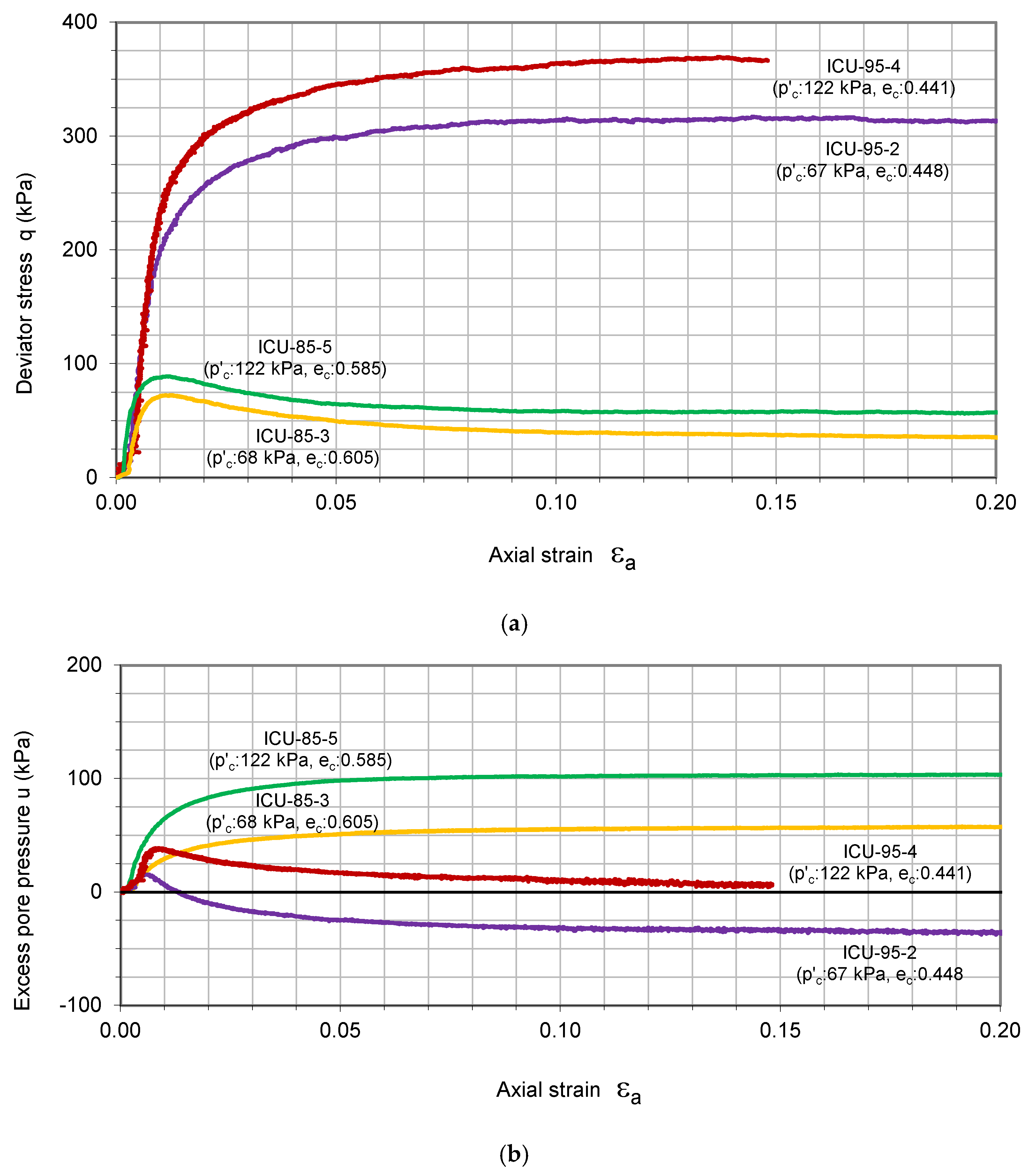
The results of deviator stress and pore pressure vs. axial strain for two pairs of tests (ICU-85-3 and ICU-95-2 consolidated to the same pressure of about 68 kPa, and ICU-85-5 and ICU-95-4 consolidated to the same pressure of about 122 kPa) are shown in Figure 3. All the test results were corrected for membrane effects according to Germaine and Ladd [9]. The consolidation pressures and void ratios of the specimens after the consolidation are also shown in the figure. The stress–stain curves showed that specimens with void ratios of 0.585 and 0.605 (ICU-85-3 and ICU-85-5) reached peak states at an axial strain of about 1% and exhibited strain-softening behavior, and pore pressures increased steadily. Both the deviator stress and the induced pore pressure reached steady states at axial strains of about 20%. Specimens with void ratios of 0.441 and 0.448 (ICU-95-2 and ICU-95-4) exhibited strain-hardening behavior with a steady increase in the deviator stress and a drop in the induced pore pressure after an axial strain of about 1%. For the details of all the test results, readers can refer to Junaideen [10].

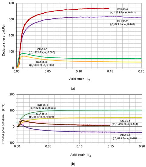
Figure 3. Results of the ICU tests on the residual soil: (a) q against ${\epsilon }_a$ ; (b) u against ${\epsilon }_a$.

3.1. Steady States

All the specimens that display strain-softening behavior reached steady states at axial strains of about 20%. The final states of the specimens showing strain-hardening behavior also signified the steady states. There are, however, concerns with the measurements taken at the boundary of dilating specimens that are likely to have severe localized shear zones. It would therefore be prudent to use only the results of the specimens showing strain-softening behavior to obtain the steady states. The data of the steady states are shown in Table 2. The steady-state line obtained from the data can be expressed by a linear line with the slope M in the p’: q plane and by a logarithmic line in the p’: v plane in the conventional way:

$$\frac{q_{ss}}{p_{ss}^{\text{'}}}=M$$

(1)

$$p_{ss}^{\text{'}}=\exp \left(\frac{\Gamma -{\nu }_{ss}}{\lambda }\right)$$

(2)

The steady-state parameters M, Γ, and λ obtained for the residual soil are given in Table 4 along with those obtained for similar soil types found in Hong Kong [11].

Table 4. Comparison of index and steady-state parameters of residual soils.

Samples		Particle Size Distribution (%)				Liquid Limit (%)	Plastic Limit (%)	Proctor Test		Steady State
		Gravel	Sand	Silt	Clay			(Mg/m3)	(%)	M	Γ	λ
Present study	Beacon Hill	35	55	8	2	45	30	1.90	12.5	1.52	1.835	0.071
Zhai (2000)	Valley Road Estate	24	54	14	8	39	29	1.78	16.0	1.61	1.818	0.049
	Chi Lin Ching Yuen	27	36	9	28	78	36	1.72	17.0	1.51	2.043	0.098
	Diamond Hill	33	49	7	11	59	31	1.70	19.0	1.62	2.223	0.111

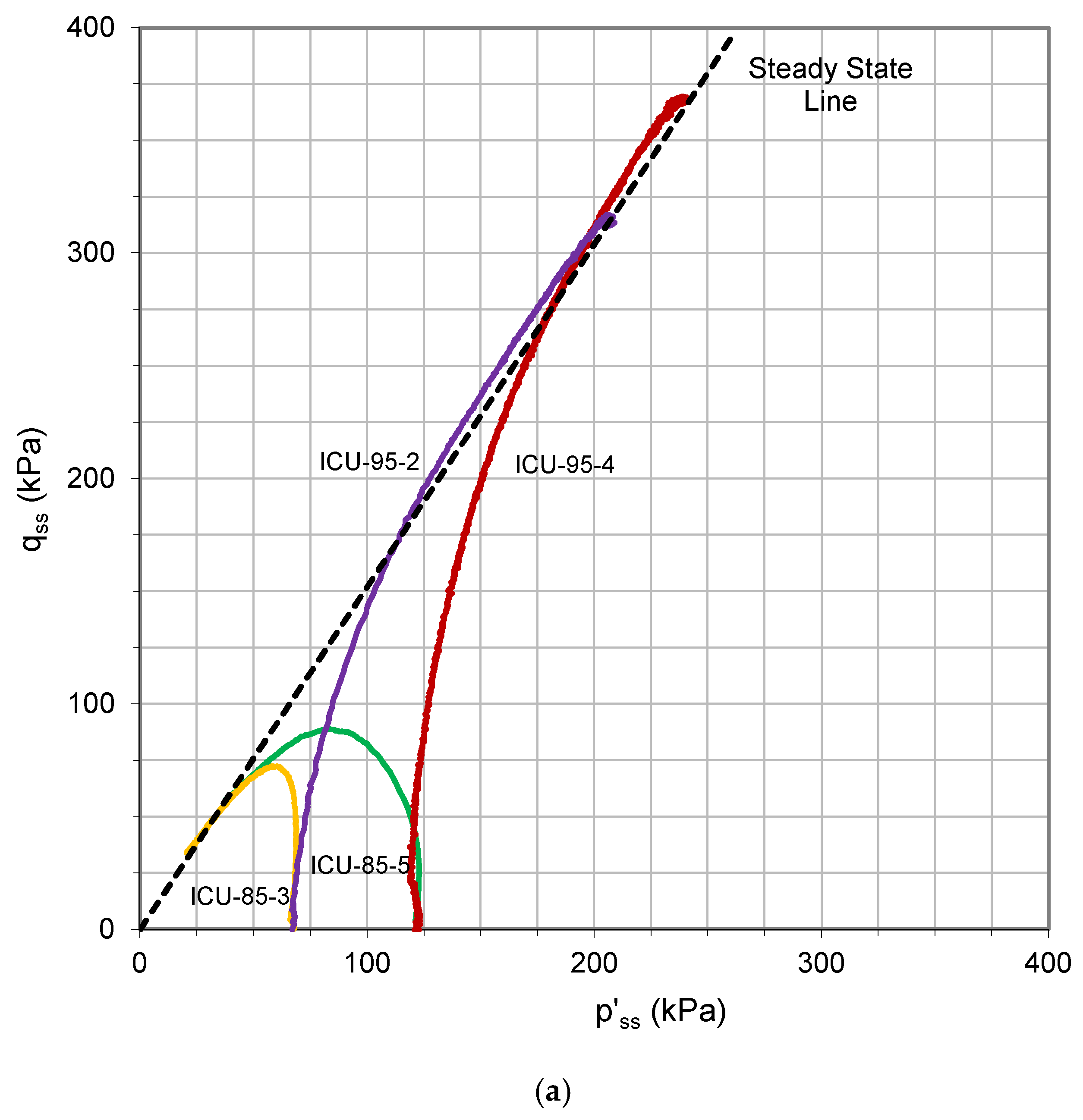
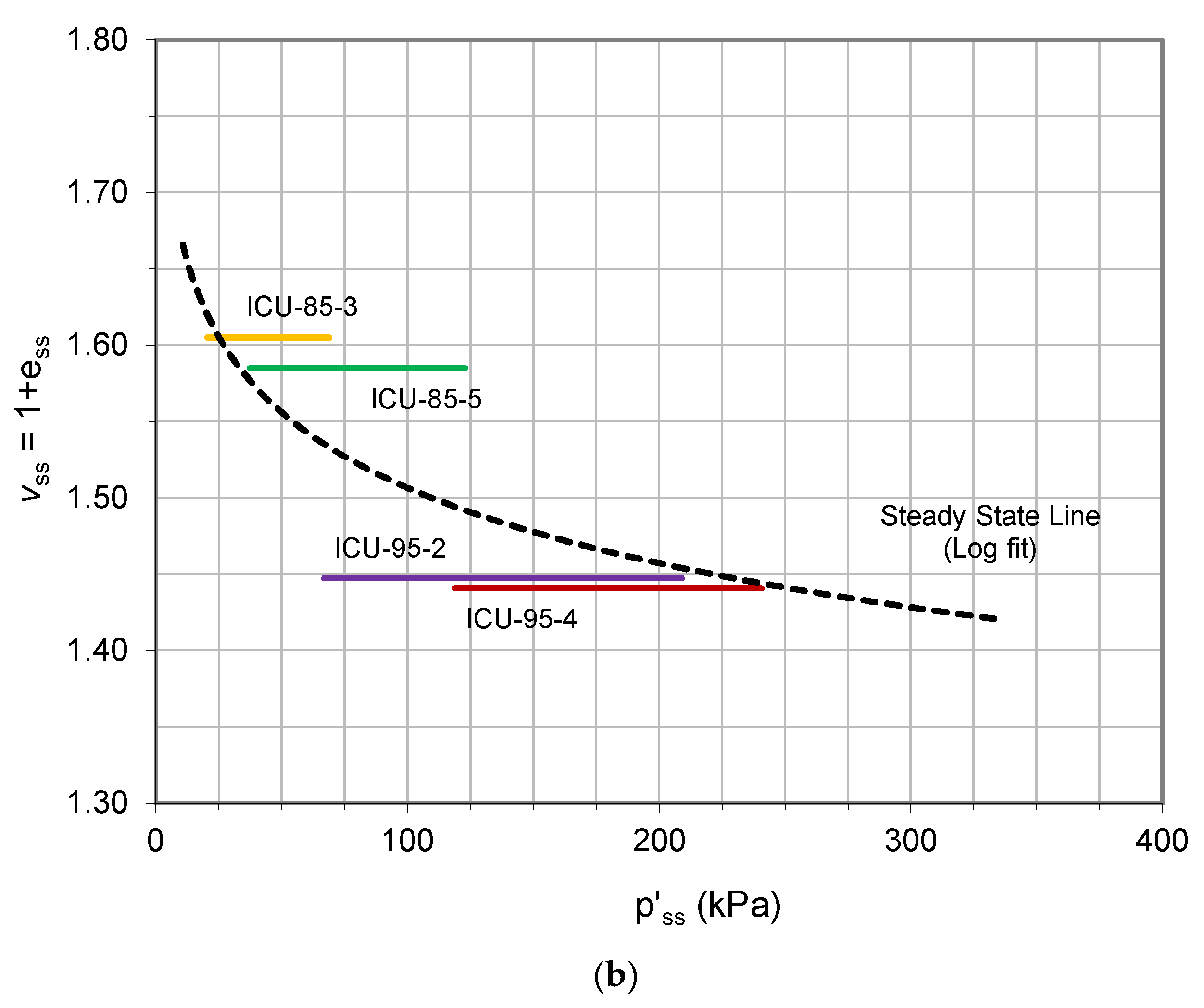
The paths in the p’: q and p’: v planes for the tests ICU-85-3, ICU-95-2, ICU-85-5, and ICU-95-4 are presented in Figure 4 together with the steady-state line. The specimens that showed strain-softening and strain-hardening behavior had their initial states, respectively, above and below the steady-state line in the p’: v plane. Furthermore, the results of the specimens that showed strain-hardening behavior approached the steady-state line at high stress levels. This validates the extension of the logarithmic relationship used in the p’: v plane to other high stress levels.

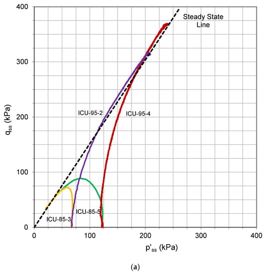
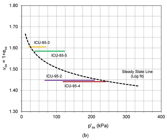
Figure 4. Stress paths for the ICU tests: (a) $p_{ss}^{\text{'}}-q_{ss}$ ; (b) $p_{ss}^{\text{'}}-v_{ss}$.

3.2. Peak States

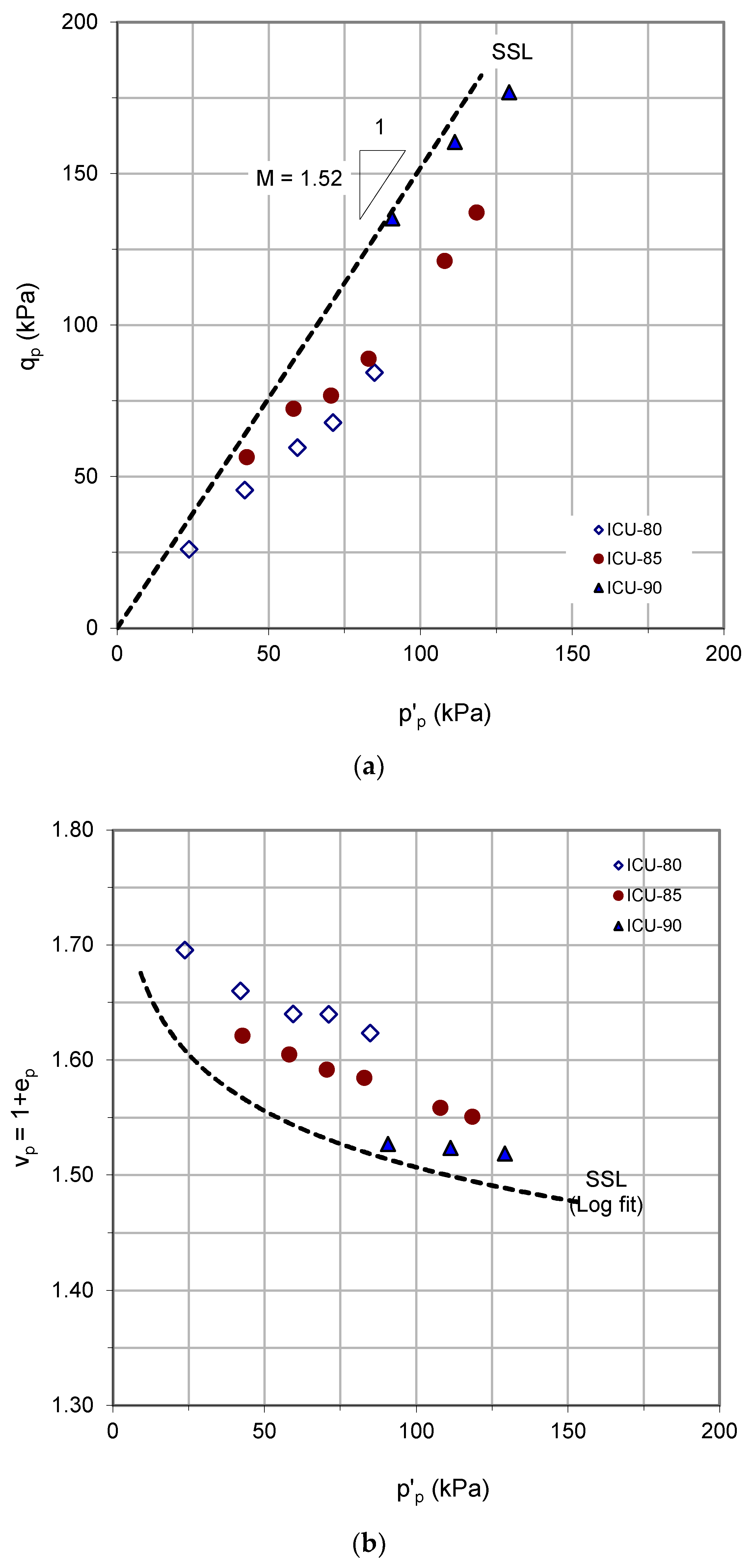
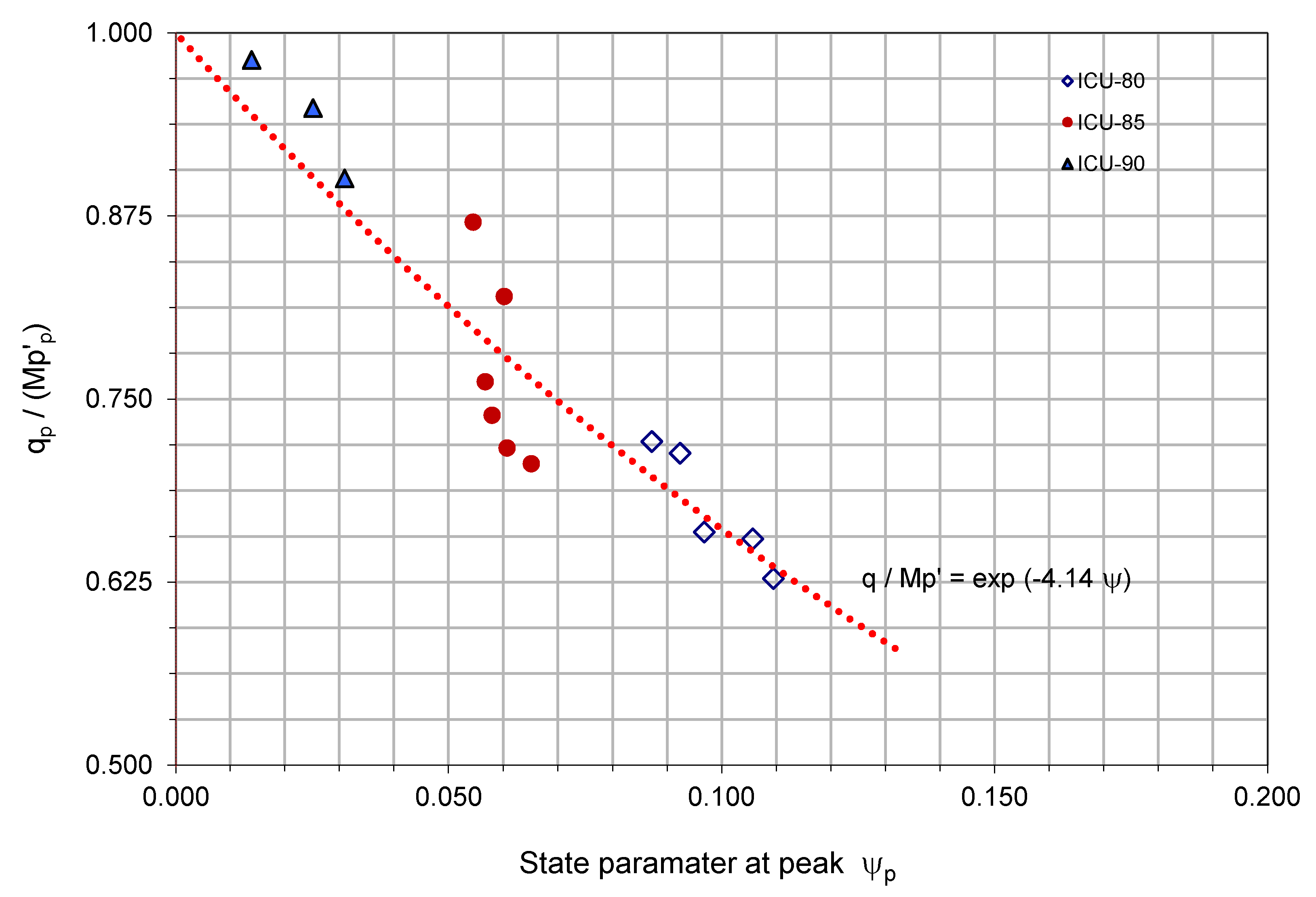
Figure 5 shows the peak states of the specimens whose initial states after consolidation were above the steady-state line in the p’: v plane. As both specific volume and stress level influenced the peak states, the soil state relative to the steady-state line in the p’: v plane could be related to the peak state. The soil state relative to the steady-state line can be defined uniquely in terms of the difference between the current specific volume $(v)$ and the specific volume at the steady-state line corresponding to the current effective stress p’ ($v_{ss}$ at p’). This difference was denoted $\psi$ and called the ‘state parameter’ by Been and Jefferies [12]. Figure 6 presents the variation in normalized peak stress ratio against the state parameter at the peak state. The results show that the peak stress ratio had a clear trend with the state parameter. A similar trend was observed by Been and Jefferies [12] and Yang [13]. The correlation between peak stress ratio and state parameter in Figure 6 can be approximated by an exponential function,

$$\frac{q_p}{M{p}_p^{\text{'}}}=\exp [-{\alpha }_u{\psi }_p]$$

(3)

where ${\alpha }_u$ is a positive constant. For the residual soil, ${\alpha }_u$ is equal to 4.14. The subscripts ‘p’ and ‘u’ denote, respectively, peak state and undrained condition. State parameter ${\psi }_p$ can be expressed as,

$${\psi }_p=v_p-(\Gamma -\lambda \ln p_p^{\text{'}})$$

(4)

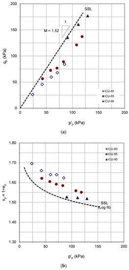
Figure 5. Peak states of the ICU results of the loose specimens: (a) $p_p^{\text{'}}-q_p$ ; (b) $p_p^{\text{'}}-v_p$.

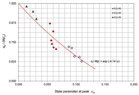
Figure 6. Peak state stress ratio as a function of state parameter.

Substituting this relation in Equation (3), the relationship between p’, q, and v at the peak states of the undrained paths can be obtained,

$$q_p=M{(p_p^{\text{'}})}^{1-{\alpha }_u\lambda }\exp [-{\alpha }_u(v_p-\Gamma )]$$

(5)

Equation (5) represents a surface in p’: q: v space that passes through the steady-state line. The equation could be written in general form omitting the subscript ‘p’.

$$q=M{(p^{\text{'}})}^{1-{\alpha }_u\lambda }\exp [-{\alpha }_u(v-\Gamma )] \mathrm{for} v\le \Gamma -\lambda \ln p$$

(6)

Unlike the collapse surface defined by Sladen et al. [1], which has a constant gradient, this surface has a gradient that varies with stress levels and specific volumes, and here, it is called the ‘modified collapse surface.’ At a particular specific volume, this becomes a curve as a function of p’. The stresses at the steady-state line corresponding to the current specific volume could be used to normalize the modified collapse surface so that it could be represented in two-dimensional form:

$$p_{ss}^{\text{'}}=\exp \left(\frac{\Gamma -\nu }{\lambda }\right)$$

(7)

$$q_{ss}=M{p}_{ss}^{\text{'}}=M\exp \left(\frac{\Gamma -\nu }{\lambda }\right)$$

(8)

This normalization technique was also used by Sladen and Oswell [14]. From Equations (6) and (8), the following equation relates the peak states of undrained loading to the steady states

$$\frac{q}{M{p}_{ss}^{\text{'}}}={\left[\frac{p^{\text{'}}}{p_{ss}^{\text{'}}}\right]}^{a_u} \mathrm{for} v\le \Gamma -\lambda \ln p$$

(9)

where $a_u=1-{\alpha }_u\lambda$, and the subscript ‘u’ denotes undrained loading

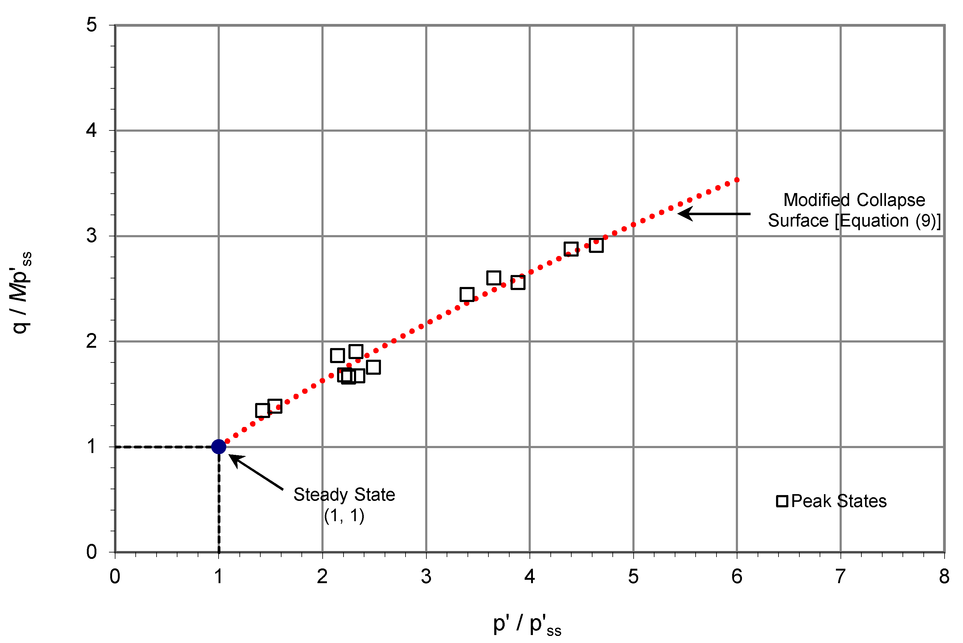
This follows that in normalized $(p^{\text{'}}/p_{ss}^{\text{'}}):(q/M{p}_{ss}^{\text{'}})$ space, all the curves corresponding to different specific volumes reduce to a single curve; and all the steady states reduce to a single point. Figure 7 presents all the peak states of the ICU test results and the curve that represents the modified collapse surface. For the residual soil, ${\alpha }_u$ = 4.14 (from Figure 6) and $a_u$ = $1-{\alpha }_u\lambda$ = 1 − 4.14 × 0.071 = 0.706.

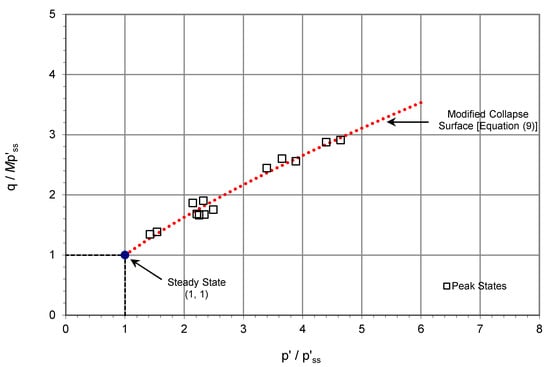
Figure 7. Modified collapse surface from the peak states of ICU results.

3.3. Post-Peak States

The undrained effective stress paths can be presented in the normalized space, see Figure 8. For clarity, not all the stress paths are shown in the figure. As proposed by Sasitharan et al. [6], the planar envelope composed of post-peak portions of the undrained effective stress paths can be delineated in the normalized space. The gradient of the planar surface in the normalized space will be $S_{pp}/M$, where $S_{pp}$ is the gradient of the planar envelope in the p’: q plane. As it passes through the steady state (1,1), the envelope can be readily defined as

$$\frac{q}{M{p}_{ss}^{\text{'}}}=\frac{S_{pp}}{M}\left(\frac{p^{\text{'}}}{p_{ss}^{\text{'}}}\right)+\left(1-\frac{S_{pp}}{M}\right)$$

(10)

where $S_{pp}=1.30$ for the residual soil. The modified collapse surface is also shown in Figure 8 for comparison.

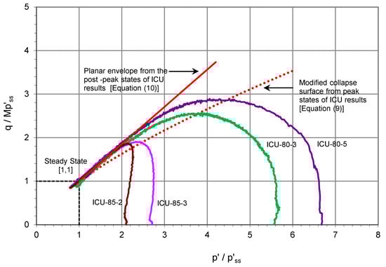
Figure 8. Normalized stress paths of the ICU results with the modified collapse surface and planar envelope.

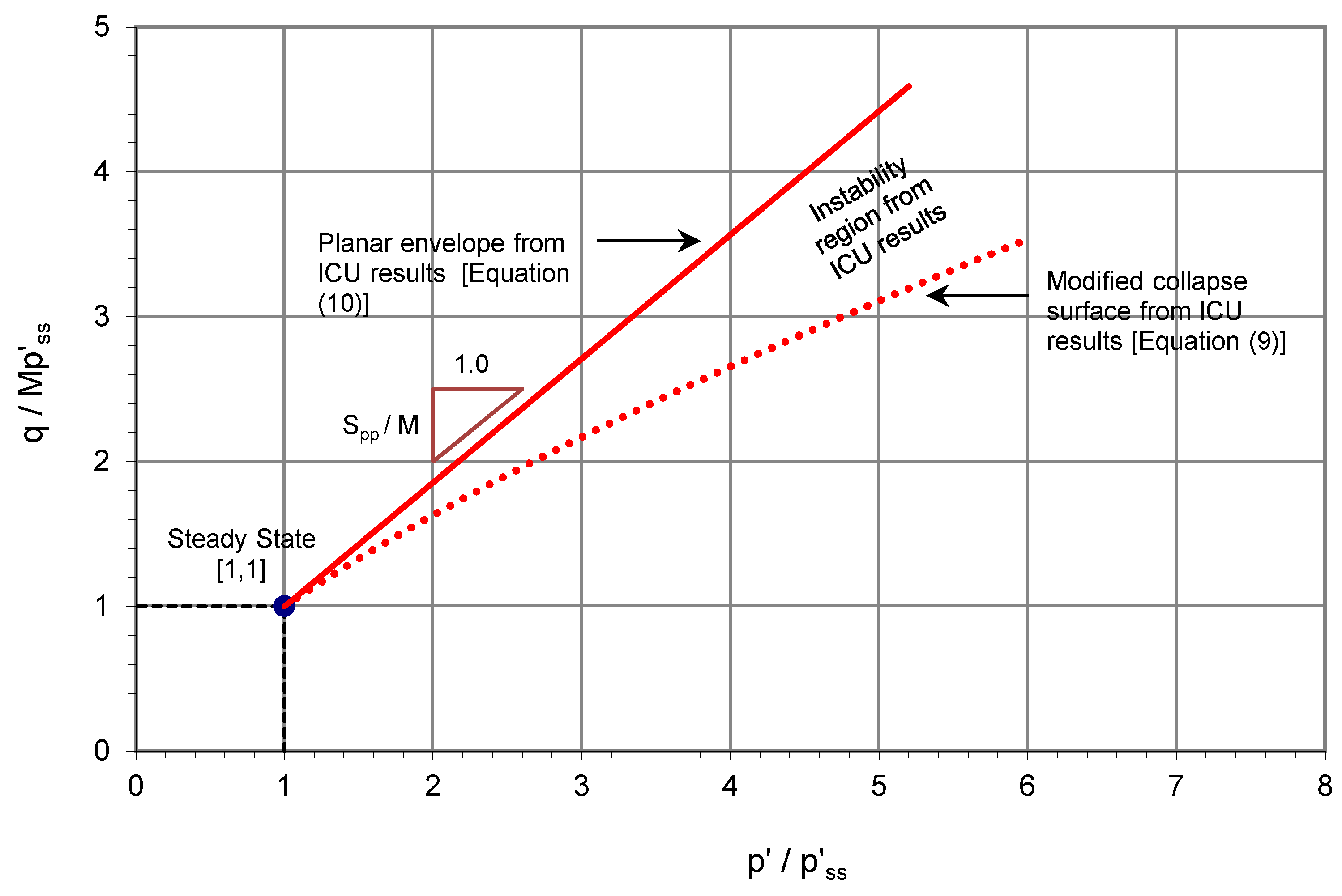
3.4. Instability Region from the ICU Test Results

Instability is perceived as the inability of a material to sustain the current stress state, resulting in large strains. Lade [15] proposed that instability is not synonymous with failure, although both lead to catastrophic events. Two failure criteria are commonly used to interpret triaxial results: ${({\sigma }_1^{\text{'}}-{\sigma }_3^{\text{'}})}_{\max }$ and ${({\sigma }_1^{\text{'}}/{\sigma }_3^{\text{'}})}_{\max }$. The two conditions are reached simultaneously in conventional drained tests. In undrained triaxial tests on loose materials, ${({\sigma }_1^{\text{'}}-{\sigma }_3^{\text{'}})}_{\max }$ is however reached before ${({\sigma }_1^{\text{'}}/{\sigma }_3^{\text{'}})}_{\max }$ is reached. Lade [15] suggested that ${({\sigma }_1^{\text{'}}-{\sigma }_3^{\text{'}})}_{\max }$ does not correspond to a true failure condition, but rather to a condition of minimum stress difference at which instability may develop inside the true failure surface. As this instability occurs before the stress state reaches the failure line [16,17,18,19], it is referred to as ‘pre-failure instability.’

Accordingly, the modified collapse surface provides the lower limit of the instability region. Besides, Sladen et al. [1] proposed that all soil states on or above the collapse surface are susceptible to liquefaction during static loading. Sasitharan et al. [5,6] suggested that the planar envelope for the post-peak portions of undrained paths defines the state boundary surface; and liquefaction can be initiated when the stress path followed during either drained or undrained loading approaches the state boundary. From the above concepts, it can be deduced that the region confined by the modified collapse surface and the planar envelope would represent unstable states for the residual soil (Figure 9). The instability region, which was obtained from the ICU test results, is examined below together with the results of the CS tests.

Figure 9. Instability region in normalized space from the ICU test results.

4. CS Test Results

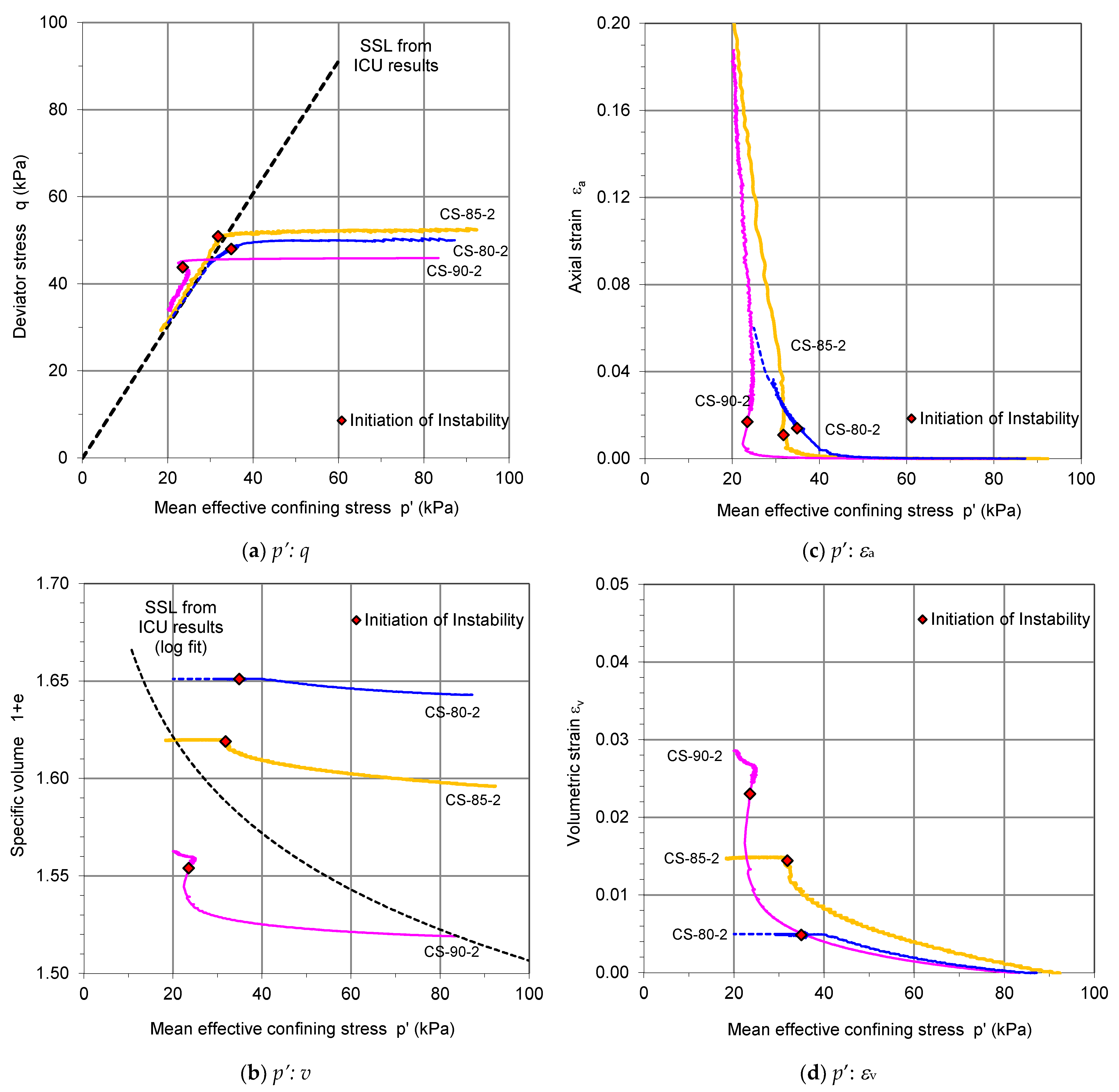
For the CS tests, three sets of specimens prepared at different relative compactions were used (refer to Table 3). Typical test results selected from each set (CS-80-2, CS-85-2, and CS-90-2) are presented in Figure 10. These specimens were isotropically consolidated approximately to p’ of 70 kPa and deviator stress was applied in a drained manner until the stress ratio (q/p’)_ac reached a value of about 0.56. The void ratios of the specimens after the anisotropic consolidation were respectively 0.643, 0.596, and 0.519. In Figure 10a–d, deviator stress q, specific volume v = 1 + e, axial strain ${\epsilon }_a$, and volumetric strain ${\epsilon }_v$ are plotted against mean effective confining stress p’. For the calculation of the volumetric and axial strains, the state after the anisotropic consolidation was considered as the initial state. Note that for CS-80-2 and CS-85-2, the initial states were well above the steady-state line in the p’: v plane, and for CS-90-2, the initial state lay on the steady-state line. For the details of the test results, readers can refer to Junaideen [10,20].

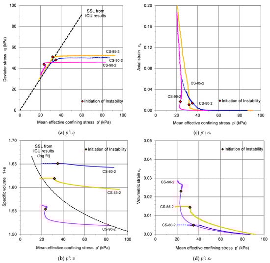
Figure 10. Typical results of the CS tests on the residual soil (a) p’: q, (b) p’: v, (c) p’: ε_a, and (d) p’: ε_v.

4.1. Initiation of Instability

For the CS tests, during the reduction in p’, volumetric strain increased consistently, whereas the axial strain started to develop only after p’ reduced below 50 kPa (Figure 10c,d). Axial strain rate increased with deceasing p’, which consequently resulted in instability of the soil specimens. The ‘initiation of instability’ is defined here using an axial strain vs. time curve: the state at which the curve deviates from the tangent drawn at 1% axial strain. For the tests shown in Figure 10a–d, the initiation of instability occurred at an axial strain between 1% and 2%.

Subsequent to the initiation of instability, the specimens CS-80-2 and CS-85-2 experienced rapid deformation and a sudden increase in pore pressures. The pore pressure readings taken at both ends of each specimen were essentially the same even during the rapid deformation, indicating uniform pore pressure distribution along the height of the specimen. For the specimen CS-90-3, which had a higher density, the initiation of instability occurred only after the volumetric strain had increased substantially. The subsequent deformation was very slow compared to those of CS-80-2 and CS-85-2, causing a slight reduction in pore pressure with a clear indication of a dilative behavior of the specimen.

4.2. Mobilized Stress Ratios

The most significant observation in the CS test results is that the initiation of instability for the loose specimens, CS-80-2 and CS-85-2, did not occur at low stress ratios as expected (Figure 10a). The mobilized stress ratios corresponding to the instability states were comparable to the steady-state stress ratios, while the associated soil states in the p’: v plane were still above the steady-state line (Figure 10b). The dense specimen CS-90-2 mobilized a stress ratio that was higher than the steady-state stress ratio; and the initiation of instability occurred after the maximum stress ratio was mobilized (Figure 10a).

4.3. Pre-Failure Instability vs. Post-Failure Instability

The initiation of instability in CS-80-2 and CS-85-2 corresponds to the ‘pre-failure instability’ state or ‘collapse’ state of the soil. The specimens could not sustain the current deviator stress and the instability led to large deformations. In the case of CS-90-2, the observed initiation of instability did not indicate such a ‘collapse’ of the specimen. In view of the fact that the phenomenon in ‘dense’ soils occurs after the failure line is reached, it is referred to as a ‘post-failure instability’ [17].

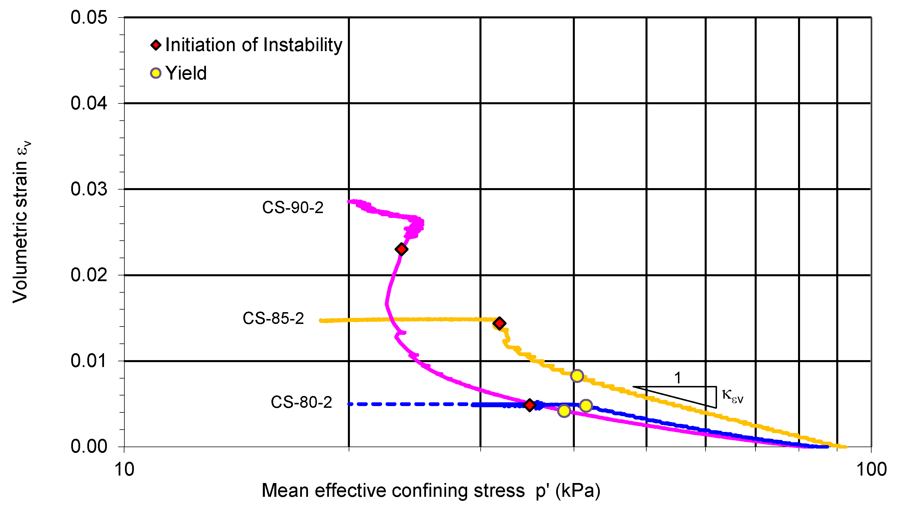
4.4. Demarcation of Yield

Figure 11 shows the yield points demarcated for the CS results. The gradient κ_εv of the linear portion of the curves in the Ln p’: ε_v plane can be transformed to the commonly used soil parameter κ = v_ac κ_εv, where κ is the gradient of the unloading line in the Ln p’: v plane, and v_ac is the specific volume of the specimen after anisotropic consolidation. The values of κ are 0.011, 0.011, and 0.008, respectively, for CS-80-2, CS-85-2, and CS-90-2. Figure 11 also indicates that between the yield state and initiation of instability, CS-90-2 exhibits significant dilation. CS-80-2 exhibits contraction, while CS-85-2 exhibits a certain degree of dilation before its initiation of instability.

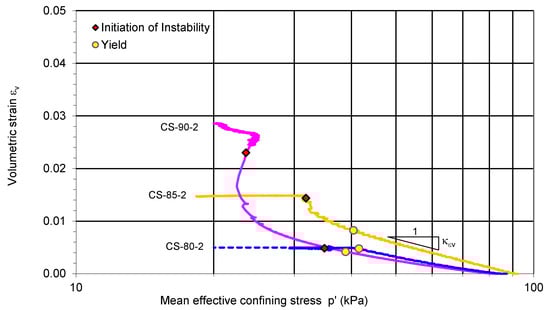
Figure 11. Yield states of the CS tests.

4.5. Normalized CS Results and Comparison with ICU Results

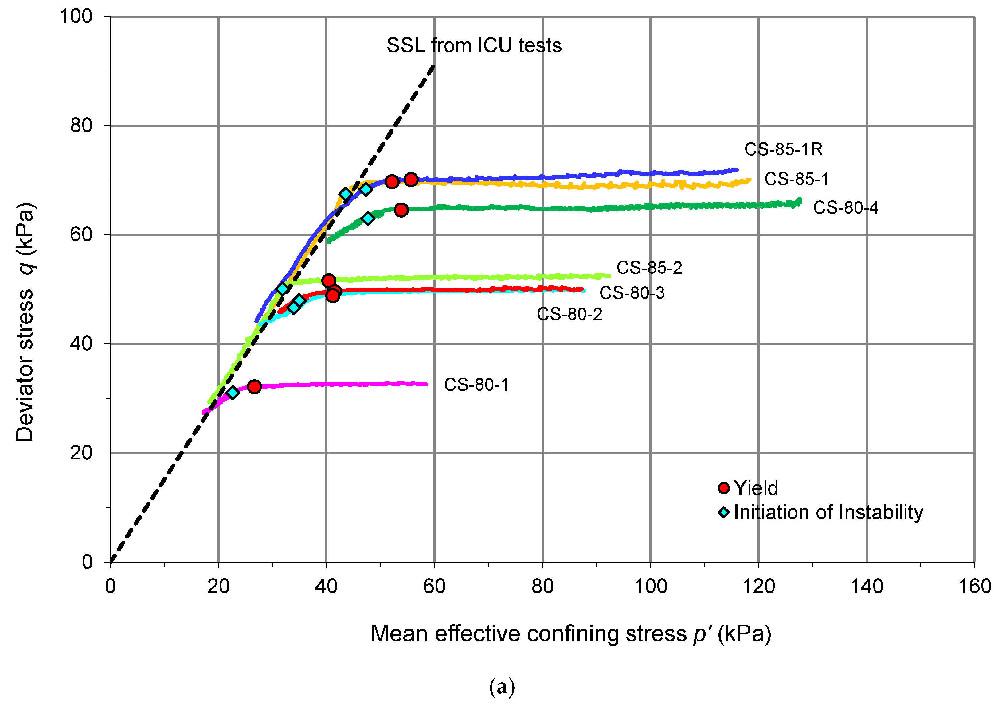
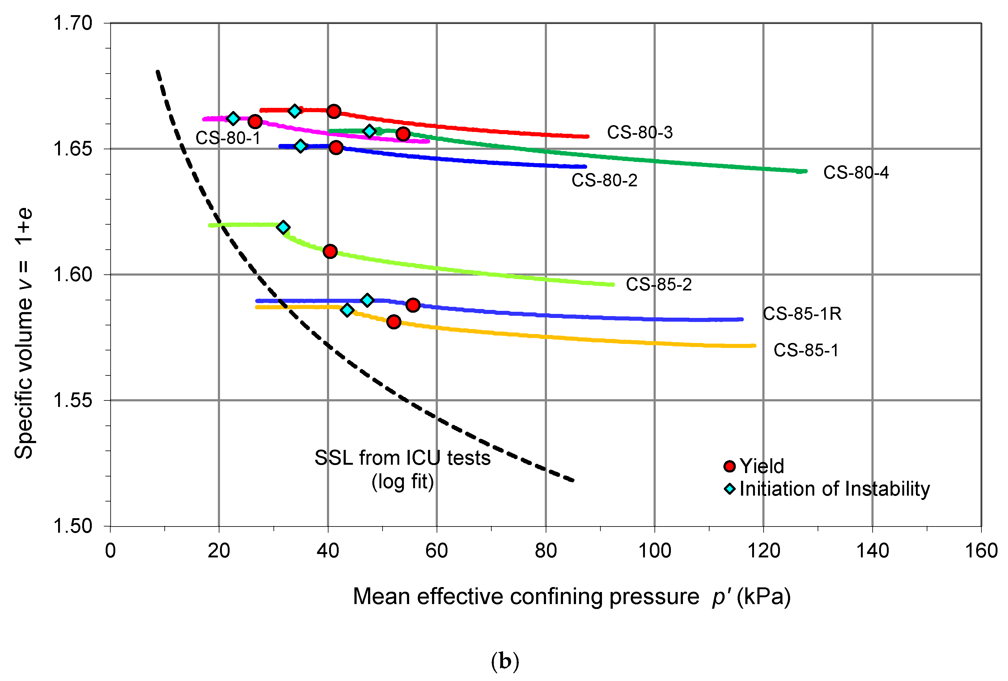
A summary of all the CS test results is given in Table 5. Figure 12 shows the results of the specimens that experienced pre-failure instability in the CS tests and the steady-state line obtained from the ICU tests. The states of yield and initiation of instability in the CS tests are also shown.

Table 5. Summary of constant shear (CS) stress test results.

Test	Initial State		Elastic Unloading		Yield State		Initiation of Instability (for Static Loading)
	${\mathit{\psi }}_{\mathit{a}\mathit{c}}$	(q/p’)ac	$\mathit{\kappa }$	$\mathit{\lambda }/\mathit{\kappa }$	${\mathit{\psi }}_{\mathit{y}}$	(q/Mp’)y	${\mathit{\psi }}_{\mathit{i}\mathit{s}}$	(q/Mp’)is	${\mathit{\epsilon }}_{\mathit{i}\mathit{s}}(\%)$
CS-80-1	0.107	0.57	0.011	6.5	0.060	0.80	0.050	0.91	1.2
CS-80-2	0.127	0.57	0.011	6.7	0.082	0.79	0.070	0.90	1.3
CS-80-3	0.139	0.57	0.013	5.6	0.095	0.78	0.082	0.91	1.4
CS-80-4	0.151	0.52	0.018	4.1	0.105	0.79	0.098	0.87	1.7
CS-85-1	0.077	0.59	0.013	5.5	0.028	0.88	0.020	1.01	2.2
CS-85-1R	0.087	0.61	0.011	6.3	0.040	0.83	0.030	0.95	1.5
CS-85-2	0.083	0.58	0.016	4.4	0.038	0.84	0.030	1.04	1.1
CS-85-3	0.116	0.57	0.014	5.0	0.064	0.93	0.061	1.02	1.7
CS-85-4	0.100	0.58	0.014	5.3	0.049	0.88	0.043	0.97	1.3
CS-85B-3	0.057	0.83	0.011	6.6	0.039	0.73	0.024	0.96	-
CS-85B-4	0.075	0.88	0.011	6.4	0.052	0.84	0.042	0.99	1.1
CS-85B-5	0.080	0.88	0.011	6.3	0.054	0.88	0.049	0.93	1.1
CS-90-1	−0.028	0.56	0.007	10.2	−0.074	0.74	−0.075	1.17	1.8
CS-90-2	0.000	0.54	0.008	8.7	−0.048	0.77	−0.055	1.22	1.7
CS-90-3	0.018	0.55	0.010	7.1	−0.039	0.93	−0.041	1.17	1.3
CS-90B-1	−0.030	1.15	0.015	4.9	−0.044	0.98	−0.037	1.12	1.6
CS-90B-2	−0.037	1.05	0.012	5.9	−0.055	0.95	−0.051	1.17	1.4
CS-90B-3	−0.065	1.09	0.012	5.9	−0.080	0.94	−0.071	1.16	1.5

Notes: $\psi$ : state parameter, $\kappa$ : gradient of specific volume with respect to Ln (p’).

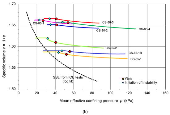
Figure 12. Results of the CS tests on the ‘loose’ specimens: (a) $p^{\text{'}}-q$ ; (b) $p^{\text{'}}-v$.

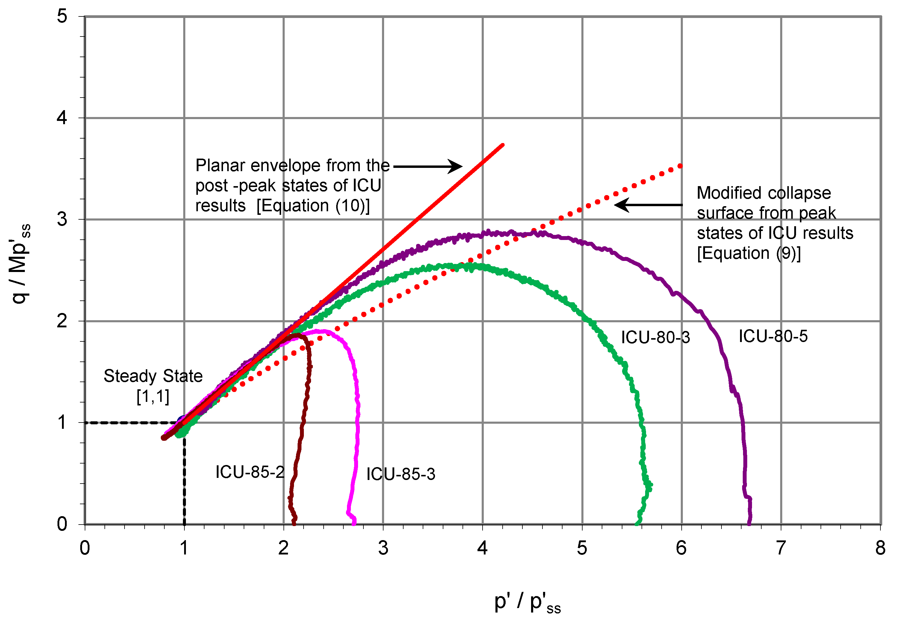
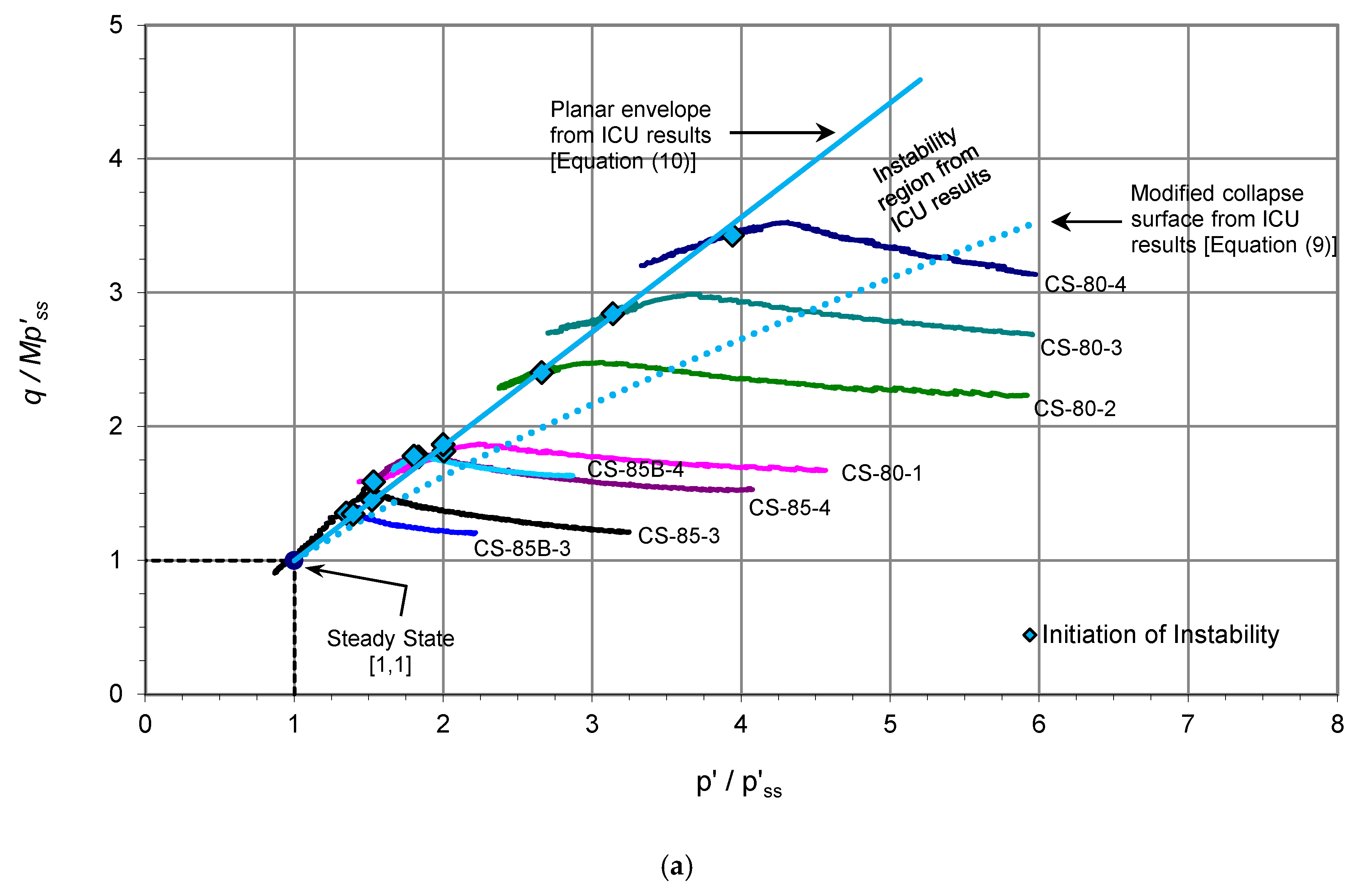
The normalized stress paths for the CS test results are shown in Figure 13a for $(p^{\text{'}}/p_{ss}^{\text{'}})\ge 1$ and Figure 13b for $(p^{\text{'}}/p_{ss}^{\text{'}})\le 1$, where $p_{ss}^{\text{'}}$ is the mean effective confining stress at the steady-state line at the current specific volume. Note that different scales have been used for these two plots. For the ICU tests, the specific volume did not change and $p_{ss}^{\text{'}}$ remained the same during the test. For the CS tests, varying specific volume caused a decrease in $p_{ss}^{\text{'}}$ during the test. The modified collapse surface and the planar envelope obtained from ICU results are also shown in Figure 13a. For clarity of presentation, not all the stress paths are shown in the figure.

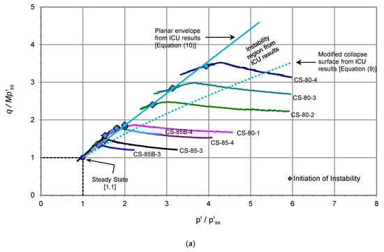
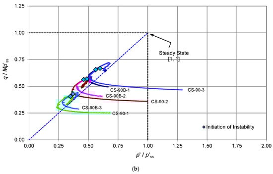
Figure 13. Normalized stress paths of CS results showing the states of ‘initiation of instability’: (a) $(p^{\text{'}}/p_{ss}^{\text{'}})\ge 1$ ; (b) $(p^{\text{'}}/p_{ss}^{\text{'}})\le 1$.

The states $(p^{\text{'}}/p_{ss}^{\text{'}})\le 1$ shown in Figure 13b represent the soil states below the steady-state line in the p’: v plane. Note that the initial state of CS-90-3 was above the steady-state line in the p’: v plane, but subsequent reduction in the effective confining stress brought the stress state below the steady-state line in the p’: v plane. For all the specimens of the CS-90 series, instability occurred after they mobilized maximum stress ratios that are higher than the steady-state stress ratio. The corresponding stress paths at the higher stress ratios appeared to trace the state boundary for the dense states of the soil.

For the loose specimens, the unstable region deduced from the ICU results was confined by the modified collapse surface (Equation (9)) and planar envelope for the post-peak states of ICU results (Equation (10)), as shown in Figure 13a. The CS results clearly show that each of the loose specimens experienced instability at a stress state falling far above the modified collapse surface. That means, before experiencing instability under the constant shear stress condition, the loose residual soil mobilized a stress ratio higher than that defined by the peak states of undrained loading. In some cases, the mobilized stress ratio was closer to the steady-state stress ratio. The results also showed that it is possible for loose soil states to exist even above the planar envelope.

4.6. Instability Surface for Static Loading

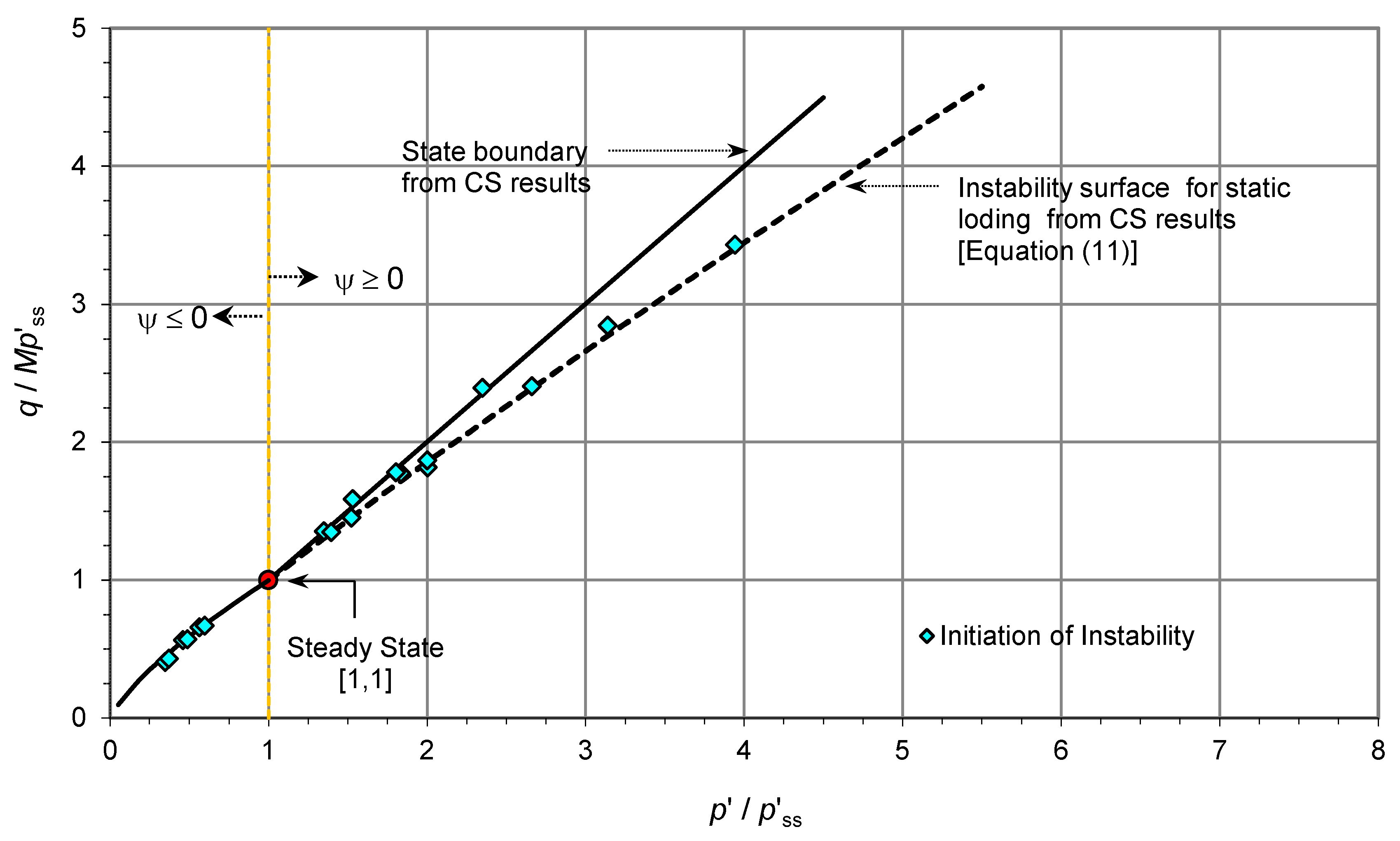
Considering the variation in the stress ratio mobilized at the initiation of instability in the CS tests with increasing density, an instability surface for static loading is postulated as a function of $(p^{\text{'}}/p_{ss}^{\text{'}})$, which uniquely defines the soil state in the p’: v plane. Figure 14 presents the postulated surface as the lower bound for the initiation of instability states in the CS tests:

$$\frac{q}{M{p}_{ss}^{\text{'}}}={\left[\frac{p^{\text{'}}}{p_{ss}^{\text{'}}}\right]}^{a_s}$$

(11)

where $a_s=0.892$ and subscript ‘s’ denotes static loading or constant shear path. With the maximum stress ratios reached in the CS tests, the state boundary is approximated to be a planar surface having a gradient of unity in $(p^{\text{'}}/p_{ss}^{\text{'}}):(q/M{p}_{ss}^{\text{'}})$ space, as shown in the figure.

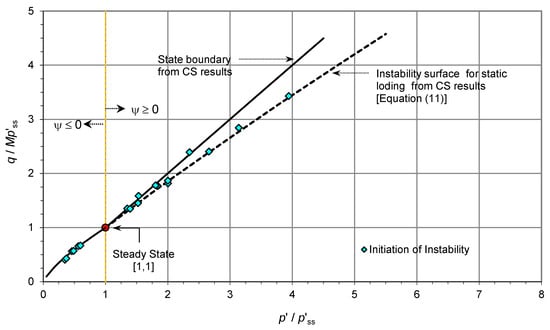
Figure 14. Instability region in normalized space from the CS test results.

5. Discussion

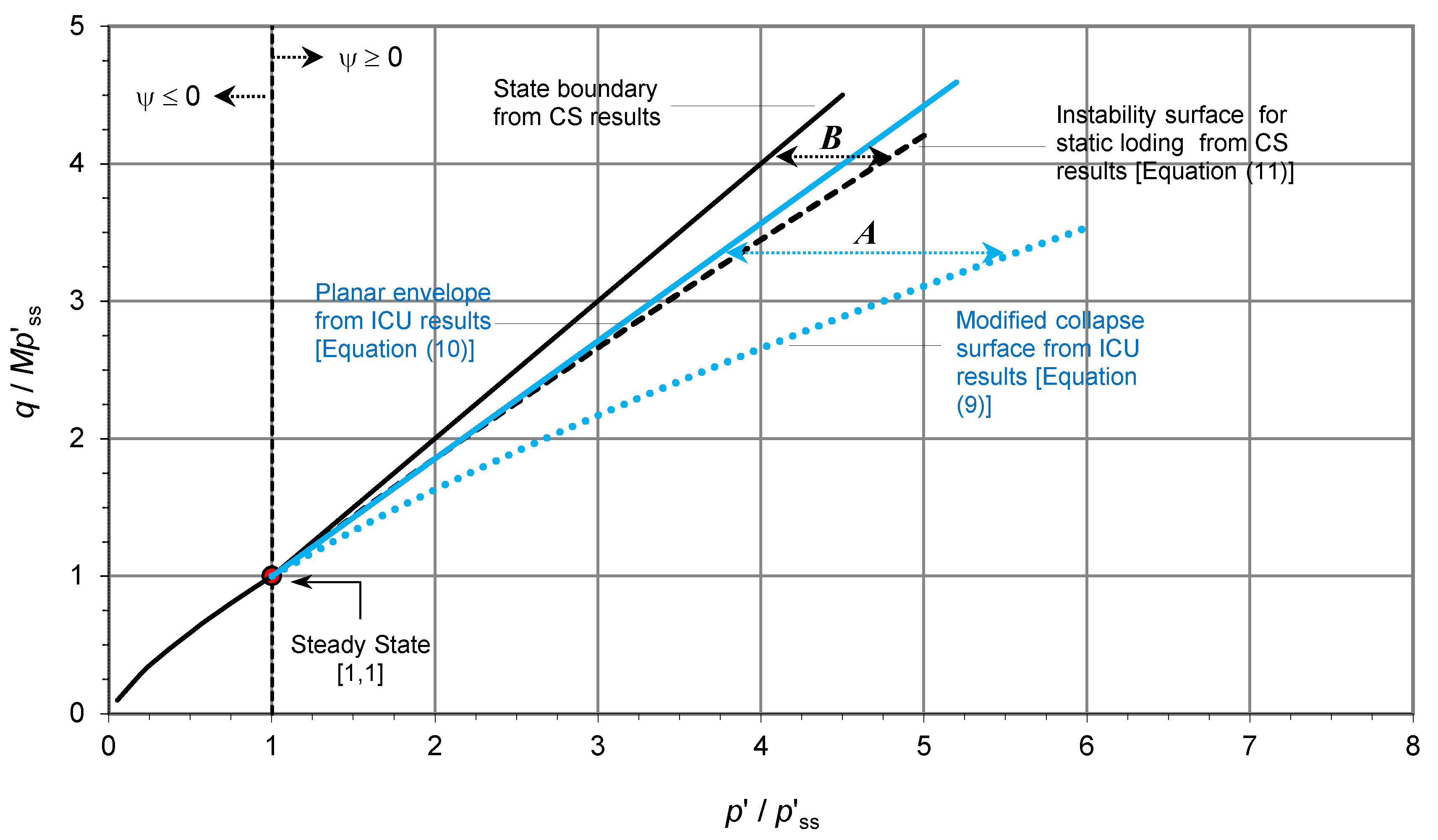
The present study allowed a systematic comparison of the results of the ICU tests and CS tests in $(p^{\text{'}}/p_{ss}^{\text{'}}):(q/M{p}_{ss}^{\text{'}})$ space in a unified manner. The instability surface and state boundary obtained from the CS results are shown in Figure 15 together with the modified collapse surface and the planar envelope of the ICU results. In the figure, the instability regions obtained from the ICU and CS results are denoted by A and B, respectively. The instability region B for static loading fell almost entirely above the instability region A for undrained loading.

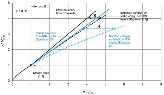
Figure 15. Comparison of the instability regions from the ICU and CS results.

The modified collapse surface defined by the peak states of undrained loading (Equation (9)) and the instability surface for static loading (Equation (11)) can be represented in a same form,

$$\frac{q}{M{p}_{ss}^{\text{'}}}={\left[\frac{p^{\text{'}}}{p_{ss}^{\text{'}}}\right]}^a$$

(12)

where $a$ = $a_u$ = 0.706 for the modified collapse surface, and $a$ = $a_s$ = 0.892 for the instability surface. The maximum stress ratio attained along the surfaces can be obtained as a function of state parameter. From Equation (12),

$$\frac{q}{M{p}^{\text{'}}}={\left[\frac{p_{ss}^{\text{'}}}{p^{\text{'}}}\right]}^{1-a}$$

(13)

But,

$$\frac{p_{ss}^{\text{'}}}{p\text{'}}=\exp \left(-\frac{\psi }{\lambda }\right)$$

(14)

From Equations (13) and (14), the maximum stress ratio can be obtained as,

$$\eta =\frac{q}{p^{\text{'}}}=\hspace{0.17em}M\exp \left[-\left(1-a\right)\frac{\psi }{\lambda }\right]$$

(15)

For a particular soil state (or state parameter), the maximum stress ratio depends on parameter $a$. The value of $a$ is smaller for the modified collapse surface than for the instability surface. Therefore, liquefaction analysis based on the normally used collapse surface would provide over-conservative results for the residual soil.

The planar ICU envelope was proposed by [6] as the state boundary for ‘very loose’ sands. Although the planar envelope does not serve as the state boundary for the loose residual soil, it coincides with the instability surface for $1.0<(p^{\text{'}}/p_{ss}^{\text{'}})<2.5$. It would therefore be of interest if the planar envelope can be related to the state parameter. From Equation (10),

$$\frac{q}{M{p}^{\text{'}}}=\left(1-\frac{S_{pp}}{M}\right)\frac{p_{ss}^{\text{'}}}{p^{\text{'}}}+\frac{S_{pp}}{M}$$

(16)

From Equations (14) and (16),

$$\frac{q}{M{p}^{\text{'}}}=\left(1-\frac{S_{pp}}{M}\right)\hspace{0.17em}\exp \left(-\frac{\psi }{\lambda }\right)+\frac{S_{pp}}{M}$$

(17)

The maximum stress ratio attained along the planar envelope is

$$\eta =\frac{q}{p^{\text{'}}}=\left(M-S_{pp}\right)\exp \left(-\frac{\psi }{\lambda }\right)+S_{pp}$$

(18)

Accordingly, the effect of state parameter on the maximum stress ratio will become insignificant when the magnitude of the state parameter becomes high. Nevertheless, the maximum stress ratio attained along the instability surface (Equation (15)) will consistently decrease with state parameter. Figure 15 also shows that the difference between the planar ICU envelope and instability surface becomes larger at higher stress levels.

It should be noted that the planar ICU envelope is just an approximation to the envelope composed of the post-peak portions of the undrained effective paths. It is also possible that the exact nature of the envelope is curvilinear and, in that case, it could coincide with the instability surface. Nevertheless, it is not always viable to obtain a curvilinear envelope from undrained stress paths. Therefore, with the present findings, if the instability surface can be deduced from the normally used planar envelope of undrained stress paths, it would be of use. By equating the gradient of Equation (10) to the secant gradient of Equation (11) with respect to the steady state, the following relationship can be obtained,

$$\frac{S_{pp}}{M}\cong \left[\frac{{(p^{\text{'}}/p_{ss}^{\text{'}})}^{{\overline{a}}_s}-1}{(p^{\text{'}}/p_{ss}^{\text{'}})-1}\right] \mathrm{for} 1.0<(p^{\text{'}}/p_{ss}^{\text{'}})<2.5$$

(19)

where S_pp is the slope of the planar ICU envelope, and ${\overline{a}}_s$ is the parameter deduced from ICU results for the instability surface of static loading. From Equation (19),

$${\overline{a}}_s\cong \frac{Ln\hspace{0.17em}\left[\frac{S_{pp}}{M}\left(\frac{p^{\text{'}}}{p_{ss}^{\text{'}}}-1\right)+1\right]}{Ln\left(\frac{p^{\text{'}}}{p_{ss}^{\text{'}}}\right)} \mathrm{for} 1.0<(p^{\text{'}}/p_{ss}^{\text{'}})<2.5$$

(20)

By substituting the soil parameters M = 1.52 and S_pp = 1.30 in Equation (20), it can be derived as 0.855 < ${\overline{a}}_s$ < 0.901 for 1.0 < $p^{\text{'}}/p_{ss}^{\text{'}}$ < 2.5. Sladen et al. [1] suggested that the ‘very loose’ state corresponds to a $p^{\text{'}}/p_{ss}^{\text{'}}$ value of 2 or greater for isotropically consolidated samples. The value of ${\overline{a}}_s$ becomes 0.892 at $p^{\text{'}}/p_{ss}^{\text{'}}$ = 2. This value coincides with the constant obtained for the instability surface from the CS test results. It is therefore reasonable to use the limiting condition of $p^{\text{'}}/p_{ss}^{\text{'}}$ = 2 to calculate the value of ${\overline{a}}_s$.

The above method of deducing the instability surface for static loading can be summarized as follows: (1) the parameters M, Γ, λ, and S_pp are obtained from conventional undrained test results; (2) the parameter ${\overline{a}}_s$ is estimated from Equation (20) using the limiting condition of $p^{\text{'}}/p_{ss}^{\text{'}}$ = 2; and (3) the value of ${\overline{a}}_s$ is substituted in Equation (11) to obtain the instability surface for static loading. As this instability surface is defined for soil states with $\psi$ ≥ 0, it can be used in a unified manner for ‘very loose’ and ‘slightly loose’ materials.

6. Conclusions

Instability behavior of a compacted residual soil was investigated using a series of conventional isotropically consolidated undrained triaxial tests and a series of specially equipped constant shear stress triaxial tests. The test results were characterized by the current state parameter $\psi$ defined in the p’: v plane with respect to the steady-state line for the residual soil.

Instability states demarcated by the peak states of the undrained triaxial tests varied with specific volume and stress level. A modified collapse surface representing the instability states of undrained loading in the p’: q: v space was proposed. Unlike the normally used collapse surface for loose sands, which has a constant gradient in the p’: q plane, the modified collapse surface for the residual soil had a gradient varying with stress levels and specific volumes.

Constant shear stress tests, which closely simulate the static loading condition, showed that before experiencing instability, the loose residual soil can mobilize stress ratios higher than the corresponding ratios defined by the modified collapse surface. A curvilinear instability surface in the p’: q: v space was proposed for the instability states reached in static loading. Further, an alternative method of deducing the instability surface for static loading from the planar envelope of the undrained stress paths was presented.

As the modified collapse surface representing the instability states of undrained loading and the instability surface representing the instability states reached in static loading are directly related to the current state parameter and mean confining stress, instability analysis for the residual soils can be performed in a unified manner.

References

- Sladen, J.A.; D’Hollander, R.D.; Krahn, J. The liquefaction of sands, a collapse surface approach. Can. Geotech. J. 1985, 22, 564–578. [Google Scholar] [CrossRef]
- Eckersley, J.D. Instrumented laboratory flowslides. Geotechnique 1990, 40, 489–502. [Google Scholar] [CrossRef]
- Lade, P.V. Initiation of static instability in the submarine Nerlerk berm. Can. Geotech. J. 1993, 30, 895–904. [Google Scholar] [CrossRef]
- Dawson, R.F.; Morgenstern, N.R.; Stokes, A.W. Liquefaction flowslides in Rocky Mountain coal mine waste dumps. Can. Geotech. J. 1998, 35, 328–343. [Google Scholar] [CrossRef]
- Sasitharan, S.; Robertson, P.K.; Sego, D.C.; Morgenstern, N.R. Collapse behaviour of sand. Can. Geotech. J. 1993, 30, 569–577. [Google Scholar] [CrossRef]
- Sasitharan, S.; Robertson, P.K.; Sego, D.C.; Morgenstern, N.R. State boundary surface for very loose sand and its practical implications. Can. Geotech. J. 1994, 31, 321–334. [Google Scholar] [CrossRef]
- Bishop, A.W.; Henkel, D.J. The Measurement of Soil Properties in the Triaxial Test; Edward Arnold Publishers: London, UK, 1962; pp. 149–152. [Google Scholar]
- Brand, E.W. Some thoughts on rainfall induced slope failures. In Proceedings of the 10th International Conference on Soil Mechanics and Foundation Engineering, Stockholm, Sweden, 10–15 June 1981; pp. 373–376. [Google Scholar]
- Germaine, J.; Ladd, C. State-of-the-Art Paper: Triaxial Testing of Saturated Cohesive Soils. In Advanced Triaxial Testing of Soil and Rock; Donaghe, R., Chaney, R., Silver, M., Eds.; ASTM International: West Conshohocken, PA, USA, 1988; pp. 421–459. [Google Scholar] [CrossRef]
- Junaideen, S.M. Failure of Saturated Sandy Soils Due to Increase in Pore Water Pressure. Ph.D. Thesis, The University of Hong Kong, Hong Kong, China, 2005. [Google Scholar]
- Zhai, Y. Fundamental Shear Behaviour of Saturated Loose Fills of Completely Decomposed Rocks. Ph.D. thesis, The University of Hong Kong, Hong Kong, China, 2000. [Google Scholar]
- Been, K.; Jefferies, M.G. A state parameter for sands. Geotechnique 1985, 35, 99–112. [Google Scholar] [CrossRef]
- Yang, J. Non-uniqueness of flow liquefaction line for loose sand. Geotechnique 2002, 54, 66–68. [Google Scholar] [CrossRef]
- Sladen, J.A.; Oswell, J.M. The behaviour very loose sand in the triaxial compression test. Can. Geotech. J. 1989, 26, 103–113. [Google Scholar] [CrossRef]
- Lade, P.V. Static instability and liquefaction of loose fine sandy slopes. ASCE J. Geotechnical. Eng. 1992, 118, 51–71. [Google Scholar] [CrossRef]
- Lade, P.V.; Pradel, D. Instability and plastic flow of soils, I: Experimental observations. ASCE J. Eng. Mech. 1990, 116, 2532–2550. [Google Scholar] [CrossRef]
- Chu, J.; Lo, S.C.R.; Lee, I.K. Strain-softening behaviour of granular soil in strain-path testing. J. Geotech. Eng. 1992, 118, 191–208. [Google Scholar] [CrossRef]
- Vaid, Y.P.; Eliadorani, A. Instability and liquefaction of granular soils under undrained and partially drained states. Can. Geotech. J. 1998, 35, 1053–1062. [Google Scholar] [CrossRef]
- Picarelli, L.; Olivares, L.; Lampitiello, S.; Darban, R.; Damiano, E. The Undrained Behaviour of an Air-Fall Volcanic Ash. Geosciences 2020, 10, 60. [Google Scholar] [CrossRef] [Green Version]
- Junaideen, S.M.; Tham, L.G.; Law, K.T.; Dai, F.C.; Lee, C.F. Behaviour of recompacted residual soils in a constant shear stress path. Can. Geotech. J. 2010, 47, 648–661. [Google Scholar] [CrossRef]
Publisher’s Note: MDPI stays neutral with regard to jurisdictional claims in published maps and institutional affiliations. |
© 2021 by the authors. Licensee MDPI, Basel, Switzerland. This article is an open access article distributed under the terms and conditions of the Creative Commons Attribution (CC BY) license (https://creativecommons.org/licenses/by/4.0/).