Empirical Evidence for Latitude and Altitude Variation of the In Situ Cosmogenic ²⁶Al/¹⁰Be Production Ratio

Abstract

We assess if variations in the in situ cosmogenic ²⁶Al/¹⁰Be production ratio expected from nuclear physics are consistent with empirical data, knowledge critical for two-isotope studies. We do this using 313 samples from glacially transported boulders or scoured bedrock with presumed simple exposure histories in the Informal Cosmogenic-nuclide Exposure-age Database (ICE-D) from latitudes between 53°S to 70°N and altitudes up to 5000 m above sea level. Although there were small systematic differences in Al/Be ratios measured in different laboratories, these were not significant and are in part explained by differences in elevation distribution of samples analyzed by each laboratory. We observe a negative correlation between the ²⁶Al/¹⁰Be production ratio and elevation (p = 0.0005), consistent with predictions based on the measured energy dependence of nuclear reaction cross-sections and the spatial variability in cosmic-ray energy spectra. We detect an increase in the production ratio with increasing latitude, but this correlation is significant only in a single variate model, and we attribute at least some of the correlation to sample elevation bias because lower latitude samples are typically from higher elevations (and vice versa). Using 6.75 as the ²⁶Al/¹⁰Be production ratio globally will bias two-isotope results at higher elevations and perhaps higher latitudes. Data reported here support using production rate scaling that incorporates such ratio changes, such as the LSDn scheme, to minimize such biases.

1. Introduction

Paired-nuclide, in situ cosmogenic nuclide analyses are valuable tools for investigating complex landscape histories, including burial after and/or during exposure. In situ cosmogenic nuclides are formed in minerals at the Earth’s surface when exposed to the high-energy particle cascade produced during interactions between cosmic radiation and atmospheric gasses [1]. Differences in production and decay ratios between multiple in situ cosmogenic radionuclides are used to estimate burial/exposure durations and erosion histories—with applications ranging from non-erosive glacier histories [2,3,4], to long-term fluvial incision [5,6] and archaeological investigations [7,8,9].

An essential component of this methodology is knowing with certainty the production ratio between measured in situ cosmogenic radionuclides. While the decay rates of cosmogenic radionuclides have been empirically constrained [10,11,12], the production rates of cosmogenic nuclides, and thus their production ratios, are estimated using models of the relevant physics [13] and validated with calibration studies that rely on independent age constraints of landscape features [14,15].

Two of the most-used in situ cosmogenic radionuclides in dual-nuclide studies are ²⁶Al and ¹⁰Be. Both are produced in quartz, and their ratio has been measured since the 1980s [16]. The near-ubiquity of quartz across the world and the improved analytical precision for ¹⁰Be—and more recently ²⁶Al [17]—measurements make these nuclides the “go to” for dual-nuclide studies. The improvement in measurement precision will allow for more useful interpretation of the data, but only if the production ratio is well constrained [18].

Physics-based nuclide production models suggest that the ²⁶Al/¹⁰Be surface production ratio should decrease with elevation and increase with latitude [19,20]; however, most analyses of ²⁶Al/¹⁰Be data assume a globally constant surface production ratio. Empirical evidence from high-latitude sites [21] suggest that this assumption may not be valid. A surface production ratio that changes with latitude and/or elevation would mean that many of the studies using this dual-nuclide methodology contain systematic biases in their results because the assumed surface production ratio may differ from the actual ratio at the sampling site. As cosmogenic nuclide measurements become more precise, better constraining of the production ratio becomes more important.

Here, we assess if changes in the ²⁶Al/¹⁰Be production ratio with latitude and/or elevation are detectable in empirical data using a compilation of 313 previously published in situ ²⁶Al/¹⁰Be ratios from samples spanning a wide range of latitudes and elevations. We applied selection criteria to increase the chances that these glacially related samples have experienced simple exposure histories—that is, only one short (<25 kyr) period of exposure and no burial, so that the measured ratio (²⁶Al/¹⁰Be) represents the surface production ratio. We apply deductive statistical analyses to this compilation to determine if ²⁶Al/¹⁰Be ratio variations with altitude, latitude, and sample processing laboratory are present at a statistically significant level. This analysis allows us to test whether there are detectable production ratio variations, thus necessitating application of physics-based nuclide production models in dual-nuclide studies, or if the nominal ratio of 6.75 is suitable at all latitudes and elevations.

2. Background

2.1. In Situ Cosmogenic ²⁶Al and ¹⁰Be

In this study, we focus on the production of in situ cosmogenic ²⁶Al and ¹⁰Be in quartz. ²⁶Al and ¹⁰Be are produced primarily through spallation reactions in quartz (>95% at sea level and high latitude) with minor production from muon interactions [1,11,12]. The ratio of muonic to spallation production increases with depth below Earth’s surface [1] and decreases at higher elevations. ²⁶Al has a half-life of 0.705 million years [10] and ¹⁰Be has a half-life of 1.39 Ma [11,12].

The accuracy of measured ²⁶Al/¹⁰Be ratios as a proxy for the ²⁶Al/¹⁰Be ratio at production is controlled by both laboratory procedures and the geologic history of sample sites. Nuclides inherited from prior periods of exposure both at the surface and at depth influence the concentration of ²⁶Al and ¹⁰Be in surface samples and thus the measured ²⁶Al/¹⁰Be ratio. Muon-induced production produces relatively few nuclides but does so at a ratio higher than surface production, which is dominated by neutrons [22]. Storage of previously exposed material at depths below the penetration depth of most neutrons can lower measured ratios as ²⁶Al decays more quickly than ¹⁰Be [10].

Laboratory concerns include the measurement of cosmogenically produced isotopes (²⁶Al and ¹⁰Be) by Accelerator Mass Spectrometry (AMS), which often sets the limit on precision, and quantification of stable isotopes (²⁷Al and ⁹Be), which is critical for accuracy. Low-energy AMS machines may be unable to completely reject isobaric interferences encountered in ²⁶Al analyses, thus artificially increasing calculated ²⁶Al concentrations and the ²⁶Al/¹⁰Be ratio [23]. When complexed with fluoride during HF digestion, Al can be difficult to get back into solution, thus leading to underestimation of ²⁶Al and consequently low ²⁶Al/¹⁰Be ratios [24]. Stable beryllium is added as a carrier (isotope dilution) but stable aluminum is native to the quartz being digested, meaning that full retention and recovery of that aluminum is critical to accurately quantifying the concentration of ²⁶Al. Stable aluminum quantification errors can arise from chemical processing steps, including aliquot measurements after, rather than before, drying dissolved samples, adding sulfuric acid to digestion solutions, and systematic offsets in calibration of inductively coupled plasma optical emission spectrometers for measuring ²⁷Al concentrations [25]. Low recovery of ²⁷Al will result in lower than actual ²⁶Al/¹⁰Be ratios [24]. Significant variation in measured ²⁶Al between chemistry labs has been observed during inter-lab comparisons, and much of this variation is attributed to differences in methodology for quantifying ²⁷Al [26,27,28]. A small number of quartz mineral separates contain significant amounts of stable ⁹Be, which, if unaccounted for, would result in spuriously low ¹⁰Be concentrations and high ²⁶Al/¹⁰Be ratios, and few laboratories routinely measure beryllium in quartz [29].

2.2. Applications

Paired in situ cosmogenic ²⁶Al and ¹⁰Be are used in a wide variety of studies seeking to understand burial and erosion histories. Early applications included the history of enigmatic Libyan desert glass [16], the age of ancient glacial deposits in the Sierra Nevada mountains [30], and the glacial history of Antarctica [31]. Bierman et al. [2] demonstrated the utility of the paired-nuclide approach for calculating minimum total durations of exposure and burial for complex glacial histories in temperate regions—those involving multiple periods of advance and retreat. Investigations of complex glacial histories continue to be a common application of ²⁶Al/¹⁰Be [32,33], including cases with minimal glacial erosion due to cold-based ice cover [4,34] and glacial histories inferred from marine sediment records [35,36]. ²⁶Al/¹⁰Be has also been used to evaluate long-term erosion rates in arid regions [37], histories of tectonic uplift [38], river incision [5,6], and paleosol burial [39,40]. ²⁶Al/¹⁰Be is also used for age control in archaeological investigations of hominin evolution [7,8,9,41], providing burial ages of bones and artifacts.

2.3. Previous Constraints on ²⁶Al/¹⁰Be Production Ratio

The production ratio of ²⁶Al/¹⁰Be at Earth’s surface has been constrained in two ways: experimental measurements—sampling surfaces with ‘known’ exposure histories—and physics-based models that simulate interactions between cosmic radiation, atmospheric atoms, and terrestrial atoms in target minerals. See Corbett et al. ([21] and Table S1 therein) for a summary of these studies and the production ratios they calculated and measured.

Studies published prior to 1991 estimated an ²⁶Al/¹⁰Be production ratio of ~6.1 [30,42], which was updated to 6.75 following updates to accelerator standards and refinements of the ¹⁰Be half-life [11,12,43]. Early models of ²⁶Al and ¹⁰Be production indicated a spallation production ratio of 6.05 that did not change with elevation (latitude changes in in situ ²⁶Al production were not modelled [44]). Without robust empirical evidence to support the use of more complex numerical models for nuclide production, an ²⁶Al/¹⁰Be production ratio of 6.75 is typically assumed to be constant over all latitudes and elevations in many scaling schemes used for cosmogenic nuclide data interpretation [45].

2.4. Indication of Spatial Variability in the ²⁶Al/¹⁰Be Production Ratio

Cross-sections for nuclide production from spallation reactions suggest changes in the ²⁶Al/¹⁰Be production ratio with latitude and elevation [19,20,46,47,48]. Although ²⁶Al and ¹⁰Be are both produced in quartz at Earth’s surface primarily through spallation reactions, the cross section—or likelihood of reaction—for spallation production is different for each nuclide. ²⁶Al has a lower energy threshold for production than ¹⁰Be, so neutron fluxes with different energy spectra produce ²⁶Al and ¹⁰Be at different ratios [47,48]. Earth’s geomagnetic field deflects lower-energy components of the primary cosmic ray flux more readily at lower latitudes [46]. The energy spectrum of the secondary neutron flux that reaches Earth’s surface therefore differs with latitude, implying a lower ²⁶Al/¹⁰Be production ratio at low latitudes, where the more energetic neutron flux favors ¹⁰Be production, and a higher production ratio at high latitudes, where the less energetic neutron flux favors ²⁶Al production [19].

A similar dynamic is expected with changes in elevation due to changes in the neutron flux energy spectrum with depth in the atmosphere. The cosmogenically derived neutron flux loses energy with increasing atmospheric depth due to interactions with atmospheric gas atoms [1,42]. Thus, the ²⁶Al/¹⁰Be production ratio should be lower at high elevations, where the neutron flux has higher energy and favors ¹⁰Be production, and highest at low elevations, where the lower energy neutron flux favors ²⁶Al production [46].

3. Materials and Methods

3.1. Data Sources and Sample Selection

To determine if the assumption of a constant ²⁶Al/¹⁰Be production ratio is an oversimplification, we test for spatial heterogeneity in the ²⁶Al/¹⁰Be production ratio using previously published samples in the Informal Cosmogenic-nuclide Exposure-age Database (ICE-D; ice-d.org, n = 313; ref. [49]). Within the ICE-D database, we extracted data from ICE-D: Alpine, data from alpine glacial landforms (n = 243), and ICE-D: Calib, samples used to calibrate cosmogenic-nuclide production rates by assuming exposure ages based on other geologic constraints (n = 70). ²⁶Al and ¹⁰Be concentration measurements for all samples were normalized to the KNSTD and 07KNSTD standards, respectively [10,43]. In both sub-databases, we targeted samples that likely experienced simple exposure histories, such that all ²⁶Al and ¹⁰Be are from a single exposure extending to the present day with no nuclides remaining from periods of prior exposures. In other words, we presume that the measured ²⁶Al/¹⁰Be concentration ratios equal the ²⁶Al/¹⁰Be production ratios for the samples we selected.

We applied the following criteria: 1. We selected samples in ICE-D: Alpine with reported ²⁶Al and ¹⁰Be concentration measurements and with exposure ages under 25 ka. Querying for ages under 25 ka ensures that measured concentrations are from a single, short period of near-surface exposure. We do not include samples from Antarctica, where prolonged burial that alters measured ²⁶Al/¹⁰Be ratios is evident in many samples (e.g., [50]). 2. We extracted all sample data from ICE-D: Calib and calculated exposure ages using the reported ¹⁰Be concentrations, LSDn scaling, and the default exposure age calculator settings in version three of the online exposure age calculator described by Balco et al. [45] (i.e., without the reference production rate from the calibration site). We kept samples in our analysis if their calculated ages using these exposure age calculator settings matched the expected ages from nearby geologic calibration sites, indicating little inherited ¹⁰Be (and by association ²⁶Al) was present in these samples.

To avoid samples affected by geologic and/or laboratory processes that can skew ratios, we discarded samples from our initial query with physically unreasonable ²⁶Al/¹⁰Be ratios. To account for the inevitable scatter in ratios due to analytical uncertainty of ²⁶Al and ¹⁰Be measurements, we first fit a normal distribution to the ²⁶Al/¹⁰Be ratio uncertainties in our compilation (Figures S2 and S3) and calculate the ratio uncertainty mean and standard deviation. We use the uncertainty mean (10.1%) plus one standard deviation (9.0%) as a threshold, beyond which we deemed the ratios physically unreasonable. Applying this 19% analytical uncertainty threshold to the canonical ²⁶Al/¹⁰Be production ratio value of 6.75 gives a range of 5.47 to 8.03 for accepted ²⁶Al/¹⁰Be ratios (details in Supplement). We assume that outlier samples were affected by geologic and/or laboratory processes that skew measured ²⁶Al/¹⁰Be concentration ratios such that they do not reflect the surface production ratio. Our final tally of samples used in statistical analyses (n = 313) does not include outliers (n = 48) removed from the original ICE:D query (Figure S1).

3.2. Statistical Analyses

We use single and bi-variate linear models, Monte Carlo simulations, and analysis of variance (ANOVA) tests to determine if variations in the measured ²⁶Al/¹⁰Be concentration ratios in our compilation are correlated with elevation and/or latitude. We first divide the sample population into three latitude transects and five elevation transects to isolate latitude and elevation as variables and create sample groups for ANOVA testing. Each elevation transect is a bin of samples from similar latitudes but spanning a range of elevations, while each latitude transect is a bin of samples with similar elevations but varying latitudes (Figure 1).

We use single and bi-variate linear models to determine if there are statistically significant correlations between the ²⁶Al/¹⁰Be production ratio, latitude, and elevation. We run single regression linear models for elevation and latitude (as absolute latitude) vs. measured ²⁶Al/¹⁰Be ratios first with the entire compilation and then with samples separated into transects, calculating 95% confidence intervals, correlation coefficients (r), and p-values against a null model (no variation in production ratio) for each iteration. We assume no uncertainty on latitude or elevation measurements. The bi-variate regression model includes elevation and latitude variables and is run for the entire compilation of samples.

We run Monte Carlo analyses to assess the influence of ²⁶Al/¹⁰Be concentration ratio uncertainties on linear regressions. In each Monte Carlo analysis, we run 1000 iterations of linear regression with samples randomly adopting an ²⁶Al/¹⁰Be concentration ratio value from within their uncertainty bounds (assuming a Gaussian uncertainty distribution) in each iteration. Monte Carlo analyses allow us to constrain a population of regressions using the uncertainties on each data point, producing another type of confidence interval that incorporates data uncertainty.

To assess if ²⁶Al/¹⁰Be concentration ratios differ between transects, we perform ANOVA testing with transects as groups. If ANOVA testing indicates that one or more transect ²⁶Al/¹⁰Be concentration ratio means are different at a 5% significance level, we perform multiple pairwise comparison of the concentration ratio means [51] to determine which transects differ and the statistical significance of differences. To assess if different cosmogenic nuclide sample preparation labs have an influence on measured ²⁶Al/¹⁰Be concentration ratios, we also perform ANOVA testing with the five labs that processed the greatest number of samples in this compilation. The five labs are located at Lawrence Livermore National Laboratory (LLNL), the University of Washington (UW), the Swiss Federal Institute of Technology in Zürich (ETH), the Australian Nuclear Science and Technology Organization (ANSTO), and the Purdue Rare Isotopes Measurement Laboratory (PRIME). Together, these labs are responsible for the ¹⁰Be and ²⁶Al extraction of 70% of the samples in our compilation.

4. Results

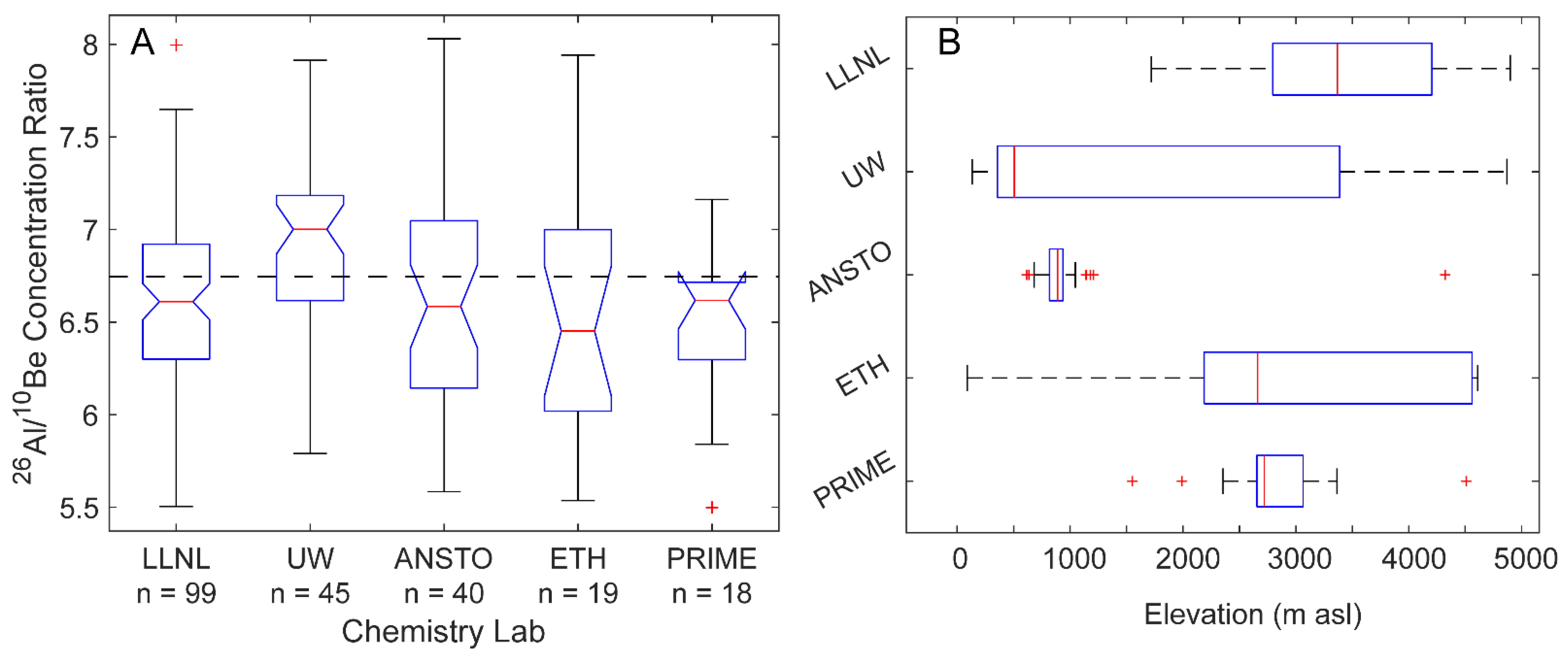
4.1. Compilation Statistics

²⁶Al/¹⁰Be concentration ratios in our sample compilation approximate a normal distribution with μ = 6.57 and σ = 0.52 (Figure 2). However, our compilation has spatial bias. While samples are present at most elevations between sea level and 5000 m asl (Figure 3B), they are biased towards the mid-latitudes in both hemispheres, with particular density around the northern mid-latitudes (Figure 3B). There are no samples from low latitude/low elevation or high latitude/high elevation locations (Figure 1). Sample processing year does not have an observable impact on the measured ²⁶Al/¹⁰Be ratio (Figure S10).

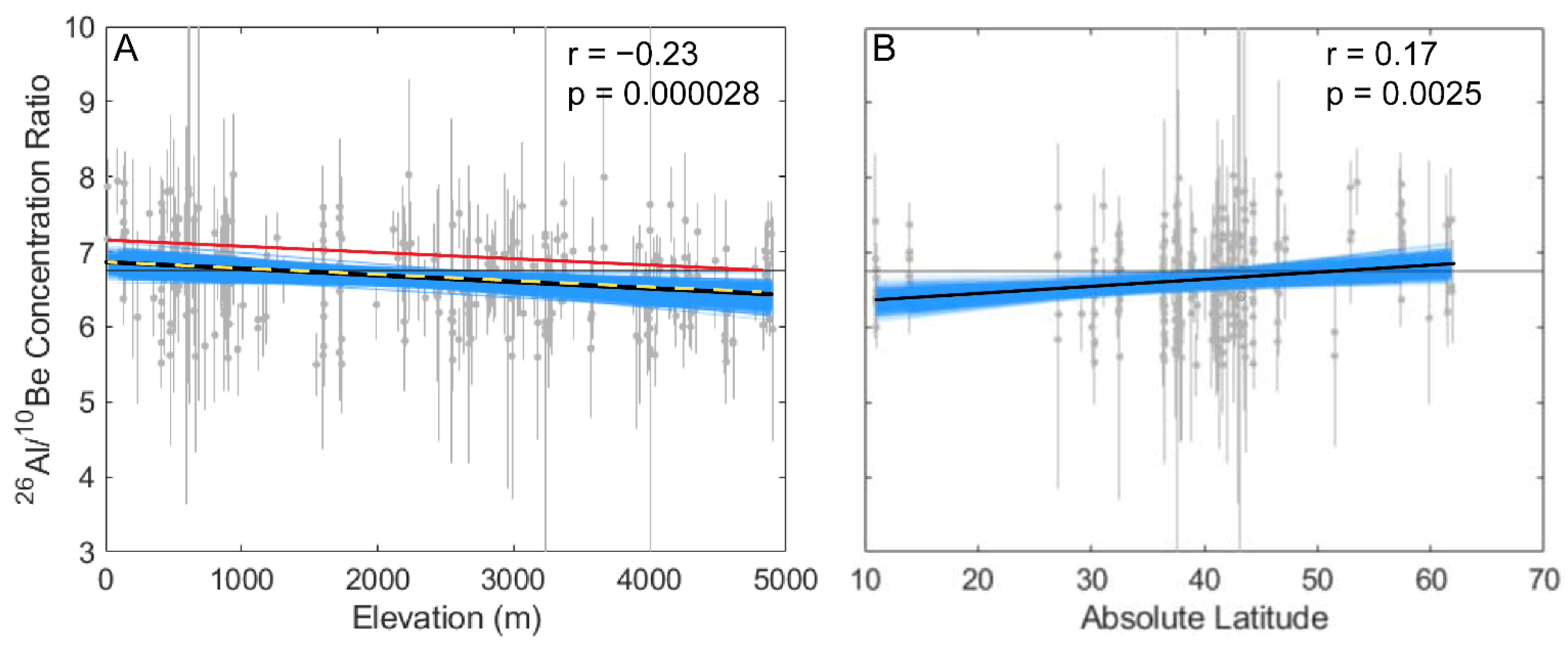
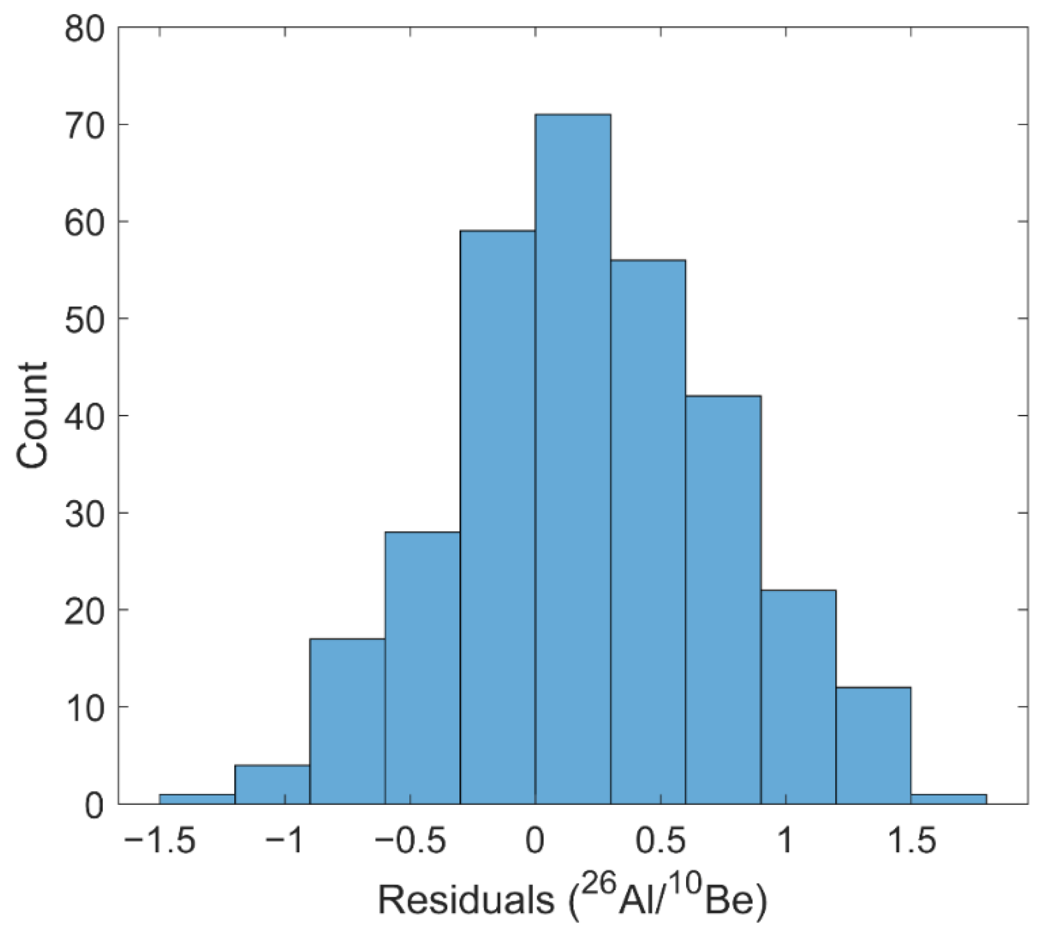
4.2. Regression Statistics

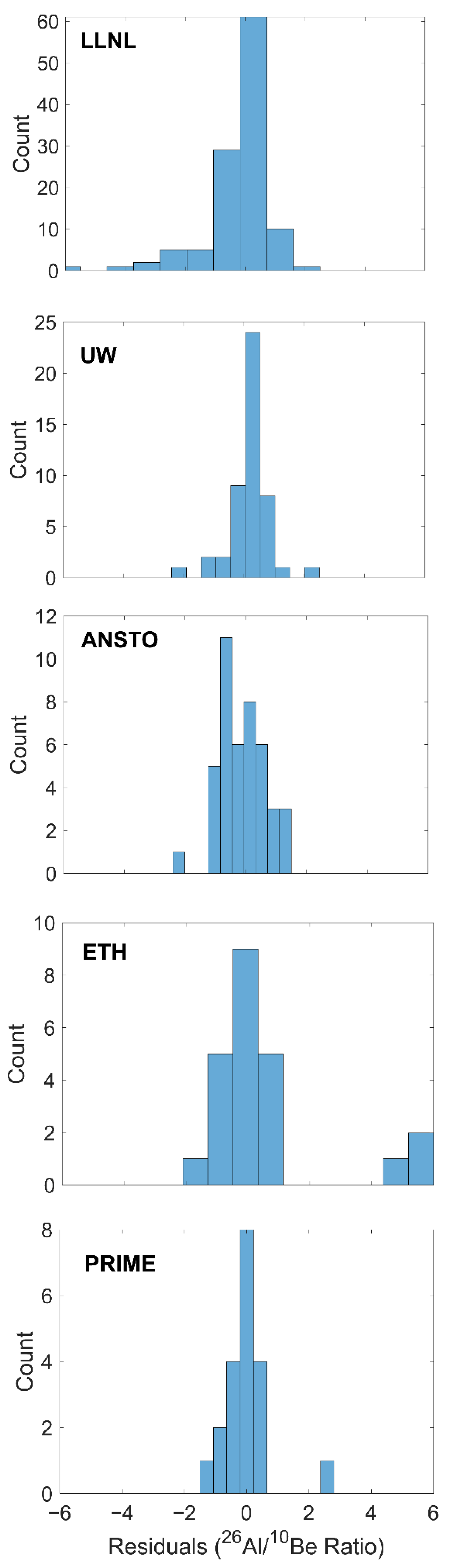
A simple linear regression of measured ²⁶Al/¹⁰Be ratios vs elevation is consistent with lowering of the ²⁶Al/¹⁰Be production ratio with elevation. The elevation regression shows a statistically significant (p = 0.000028) negative correlation (r = −0.23) between elevation and measured ²⁶Al/¹⁰Be ratios (Figure 4A). Although large, the residuals from the elevation/ratio regression are normally distributed; there is no evidence of heteroscedasticity. The regression exhibits good fit to the data, as indicated by a reduced chi-squared test, which accounts for scatter caused by uncertainty in the data (${\mathsf{\chi }}_{\nu }^2$ = 1.25). The Monte Carlo regressions support a negative correlation, with every regression exhibiting a negative slope and with the 95% confidence interval (95% of regressions) overlapping the ratio change expected with elevation in nuclide production models (change in ratio = −0.083 per km elevation, calculated from [20]).

A linear model with measured ²⁶Al/¹⁰Be ratios and latitude (as absolute latitude) supports an increase in the production ratio with increasing latitude. The latitude/ratio regression shows a statistically significant (p = 0.0025) positive correlation (r = 0.17) between latitude and ²⁶Al/¹⁰Be ratios (Figure 4B). This latitude/ratio regression has normally distributed residuals with no evidence of heteroscedasticity and exhibits good fit to the data (${\mathsf{\chi }}_{\nu }^2$ = 1.27). The 95% confidence interval of the change in ratio with latitude as provided by Monte Carlo regressions overlaps the change expected from nuclide production models (change in ratio = 0.0053 per degree latitude, calculated from [20]).

Our bi-variate linear model with elevation and latitude as variables (

Table 1. Bivariate regression statistics table with elevation and latitude as variables (y = x₁ + x₂ × elev + x₃ × lat).

	Estimate	SE	tStat	p Value
Intercept	6.86	0.24	28.26	8.74 × 10−88
Elevation	−8.97 × 10−5	3.09 × 10−5	−2.91	0.004
Latitude	−3.02 × 10−4	0.005	−0.07	0.947

F-statistic vs. constant model: 9, p-value = 0.00016.

) is a statistically significant improvement over a null model (p = 0.00016) and supports a negative correlation between elevation and ²⁶Al/¹⁰Be production ratio but does not support a positive correlation between latitude and ²⁶Al/¹⁰Be production ratio (Table 1). The bi-variate model has normally distributed residuals (Figure 2B, Figure S5), no evidence of heteroscedasticity (Figure S7), and fits the data well (${\mathsf{\chi }}_{\nu }^2$ = 1.24), offering a marginal improvement over the elevation-only regression. The change in ²⁶Al/¹⁰Be ratio with elevation in the bi-variate model is within the 95% Monte Carlo confidence range of the elevation-only model, close to the change predicted by a nuclide production model [20], and is statistically significant (p = 0.004). The change in ²⁶Al/¹⁰Be ratio with latitude in the bi-variate model is not statistically significant (p = 0.947). This model indicates that there is variation in measured ²⁶Al/¹⁰Be concentration ratios over space, and that elevation differences appear to have the strongest correlation to these changes.

Linear regressions in elevation and latitude transects support ²⁶Al/¹⁰Be ratio variations in only one transect. Measured ²⁶Al/¹⁰Be ratios in elevation transect 1 (spanning latitudes 40°–50°S; Figure 1) exhibit a statistically significant (p = 0.011) negative correlation (r = −0.34) with elevation. Correlations in every other transect are not significant at the 5% level and exhibit wide 95% confidence intervals (Figure S4).

4.3. ANOVA

ANOVA tests indicate that there is a statistically significant difference in measured ²⁶Al/¹⁰Be ratios between samples from the highest and lowest elevations. Both the mean and median ²⁶Al/¹⁰Be concentration ratio from latitude transects 1 (200 to 600 m asl) and 3 (4000 to 5000 m asl) are significantly different (p = 4.96 × 10⁻⁵; Figure 5). Moreover, the ratio differences are as predicted by nuclear physics models, with the lower elevations having a higher ²⁶Al/¹⁰Be ratio (mean ± SE = 6.80 ± 0.12, median = 6.95) than higher elevations (mean = 6.49 ± 0.11, median = 6.48, Figure 5). The mean and median ²⁶Al/¹⁰Be concentration ratio from latitude transect 2, covering the 1400 to 1800 m asl elevation band, is different than latitude transect 1 at the 5%, but not 1%, significance level (p = 0.025) and is not significantly different than latitude transect 3 (Figure 5).

Mean ²⁶Al/¹⁰Be concentration ratios from elevation transects 1 (6.76 ± 0.14) and 3 (6.45 ± 0.12), which cover 40° to 50°S and 36° to 39°N, respectively, are significantly different (p = 0.008; Figure 6). Every other elevation transect is statistically similar. Aside from transect 3, all elevation transects also have mean ²⁶Al/¹⁰Be concentration ratios that overlap the canonical value of 6.75 within the envelope of mean standard errors (Figure 6B).

Sample preparation lab ANOVA testing revealed that samples from the University of Washington Cosmogenic Nuclide Laboratory (UW) have higher mean and median ²⁶Al/¹⁰Be concentration ratios than other labs (Figure 7A). Sample ratios from UW were different than samples processed at Lawrence Livermore National Laboratories (LLNL), but not other labs, at a statistically significant level (p = 0.006).

5. Discussion

The ²⁶Al/¹⁰Be production ratio changes with elevation as numerical models of the underlying nuclear physics predict. Our analysis of 313 glacially eroded and exposed samples from around the world, for which we assume simple exposure histories, supports the calculations and conclusions of Lifton et al. [20] and Argento et al. [19]. These numerical models predict a decrease in the ²⁶Al/¹⁰Be production ratio from sea level to 5000 m asl of ~4% and 2.5%, respectively (see Figure 8 in [20]), and our ANOVA results agree well with the model predictions (4.6 ± 0.7% difference between latitude transects 1 and 3). Our bi-variate regression produces a good fit to measured ²⁶Al/¹⁰Be ratios (${\mathsf{\chi }}_{\nu }^2$ = 1.24), and the negative correlation between elevation and ratio is highly significant (Table 1).

The positive correlation between the ²⁶Al/¹⁰Be ratio and latitude is less robust in our data than the negative correlation with elevation. The statistically significant correlation observed in the latitude/ratio regression (Figure 4B) is not replicated in the bi-variate model (Table 1) and ANOVA tests are inconclusive, with only two latitude bands of the five elevation transects exhibiting a statistically significant difference in ²⁶Al/¹⁰Be (Figure 6). These two elevation transects are not substantially different in terms of absolute latitude, with transect 1 covering 40°–50°S and transect 3 covering 36°–39°N (Figure 1), and we attribute at least some of the difference in ratios to sample elevation differences between the transects. Despite the intention for transects to isolate latitude and elevation as variables, these two transects contain samples from different elevations. Samples in elevation transect 1 range from sea level to ~1500 m asl; samples in elevation transect 3 range from ~1500 to 5000 m asl. Numerical model predictions and the statistically significant elevation/ratio correlation in our analyses suggest that ²⁶Al/¹⁰Be ratios in elevation transect 1 should be several percent higher than ratios in elevation transect 3 just due to elevation differences. Thus, the 1 to 5% difference in mean ²⁶Al/¹⁰Be ratios observed between these transects in ANOVA results is at least partially due to elevation-related differences in production.

The higher ratios observed in samples processed at UW do not skew our interpretation of elevation and latitude influences on the ²⁶Al/¹⁰Be production ratio, and we attribute the higher ratios partially to differences in the elevation of samples processed in these two labs. To assess the leverage of the higher-ratio UW samples, we created a bi-variate regression model with these samples removed and found no significant difference in our results. Both the elevation/ratio correlation and the model itself were still statistically significant, although the elevation/ratio correlation was not as robust as when the UW samples are included (p = 0.02 vs. p = 0.004; Table S1). Samples processed at UW are from low elevations, with more than 50% from below 500 m asl, while the only lab with significantly different ratios, LLNL, has samples from predominantly high elevation locations (Figure 7B). The negative correlation between elevation and ²⁶Al/¹⁰Be ratios demonstrated here and predicted by Lifton et al. [20] could thus be partially responsible for the observed difference between UW and LLNL results.

Differences in sample processing techniques may also explain some of the difference in measured ratios between labs. Data from our initial query (i.e., before setting cutoff values to constrain “reasonable” ratios) show that UW has less variance in measured ²⁶Al/¹⁰Be ratios than any other chemical processing lab (relative standard deviation, RSD = 9.6% compared to RSD > 11% at other labs and 17.7% at LLNL), and all but two UW samples were within the cutoff ratio bounds. LLNL ratios from the initial query are skewed low, indicating perhaps an underestimation of native ²⁷Al in samples and thus the calculated ²⁶Al concentrations. We fit our bi-variate model to the measured ratios from each of the major chemical processing labs to assess this hypothesis and indeed found a more left-skewed residuals distribution from LLNL and a tighter fit (smaller residuals) from UW (Figure 8). Thus, we attribute the difference in measured ²⁶Al/¹⁰Be ratios between LLNL and UW to both elevation differences between samples and more variable and low-skewed ²⁶Al/¹⁰Be measurements from LLNL.

6. Implications

Our analysis suggests that dual-nuclide studies that assume a spatially invariant ²⁶Al/¹⁰Be production ratio of 6.75 contain small but systemic biases in their data interpretations. The change in the ²⁶Al/¹⁰Be production ratio (5–6% between the equator and the poles and between sea level and mountain landscapes) is similar to the current analytical uncertainty of well-measured ²⁶Al/¹⁰Be ratios. Using the nominal ratio (6.75) at high latitudes and low elevations will underestimate burial times at higher latitudes and lower elevations.

Using a nuclide-specific production rate spatial scaling model (such as the LSDn scaling scheme from Lifton et al. [20]) will improve the accuracy of dual-nuclide studies. The LSDn scaling scheme fits the ²⁶Al/¹⁰Be ratio data in this compilation nearly as well as the bi-variate regression (${\mathsf{\chi }}_{\nu }^2$ = 1.46; Figure 9, Figures S6, S8 and S9) and predicts ratio variations with elevation that are consistent with the empirical data (Figure 4A). The LSDn scaling scheme also predicts an increase in the ²⁶Al/¹⁰Be production ratio with latitude, which agrees with our single variate latitude/ratio regression but is not observed in our bi-variate regression.

Our analysis is limited by spatial gaps in the data, particularly at low latitude/low altitude and high latitude/high altitude locations and thus may be biased by elevation-dependence of sites from different latitudes. Filling these gaps is essential to improving our understanding of ²⁶Al/¹⁰Be production ratio variations, but will be challenging. Glaciers did not occupy low latitude/low altitude sites, but other episodically exposed surfaces, such as those from rock falls, could be useful. Sampling high latitude/high altitude sites is logistically difficult, and many of these sites which have been sampled show evidence for significant concentrations of nuclides inherited from prior periods of exposure.

Analysis of these compiled data indicate the need for improving the precision and accuracy of ²⁶Al/¹⁰Be measurements and thus their application to geochronology and understanding landscape dynamics. Of particular concern are measurements of stable ²⁷Al. Use of internal laboratory standards for quality control can help assure the quality of both ²⁶Al and ¹⁰Be data. These are available as liquid standards [53], homogenized glass sand powder [25], and as purified quartz [26,28]. Improved precision of ²⁶Al concentration measurements will also be critical to constraining ²⁶Al/¹⁰Be ratios [17].

References

1. Gosse, J.C.; Phillips, F.M. Terrestrial in situ cosmogenic nuclides: Theory and application. Quat. Sci. Rev. 2001, 20, 1475–1560. [Google Scholar] [CrossRef]
2. Bierman, P.R.; Marsella, K.A.; Patterson, C.; Davis, P.T.; Caffee, M. Mid-Pleistocene cosmogenic minimum-age limits for pre-Wisconsinan glacial surfaces in southwestern Minnesota and southern Baffin Island: A multiple nuclide approach. Geomorphology 1999, 27, 25–39. [Google Scholar] [CrossRef]
3. Briner, J.P.; Miller, G.H.; Davis, P.T.; Bierman, P.R.; Caffee, M. Last glacial maximum ice sheet dynamics in Arctic Canada inferred from young erratics perched on ancient tors. Quat. Sci. Rev. 2003, 22, 437–444. [Google Scholar] [CrossRef]
4. Corbett, L.B.; Bierman, P.R.; Rood, D.H. Constraining multi-stage exposure-burial scenarios for boulders preserved beneath cold-based glacial ice in Thule, northwest Greenland. Earth Planet. Sci. Lett. 2016, 440, 147–157. [Google Scholar] [CrossRef] [Green Version]
5. Granger, D.E.; Kirchner, J.W.; Finkel, R.C. Quaternary downcutting rate of the New River, Virginia, measured from differential decay of cosmogenic 26Al and 10Be in cave-deposited alluvium. Geology 1997, 25, 107–110. [Google Scholar] [CrossRef]
6. McPhillips, D.; Hoke, G.D.; Liu-Zeng, J.; Bierman, P.R.; Rood, D.H.; Niedermann, S. Dating the incision of the Yangtze River gorge at the First Bend using three-nuclide burial ages. Geophys. Res. Lett. 2016, 43, 101–110. [Google Scholar] [CrossRef] [Green Version]
7. Carbonell, E.; Bermúdez De Castro, J.M.; Parés, J.M.; Pérez-González, A.; Cuenca-Bescós, G.; Ollé, A.; Mosquera, M.; Huguet, R.; Van Der Made, J.; Rosas, A.; et al. The first hominin of Europe. Nature 2008, 452, 465–469. [Google Scholar] [CrossRef] [Green Version]
8. Gibbon, R.J.; Pickering, T.R.; Sutton, M.B.; Heaton, J.L.; Kuman, K.; Clarke, R.J.; Brain, C.K.; Granger, D.E. Cosmogenic nuclide burial dating of hominin-bearing Pleistocene cave deposits at Swartkrans, South Africa. Quat. Geochronol. 2014, 24, 10–15. [Google Scholar] [CrossRef]
9. Granger, D.E.; Gibbon, R.J.; Kuman, K.; Clarke, R.J.; Bruxelles, L.; Caffee, M.W. New cosmogenic burial ages for Sterkfontein Member 2 Australopithecus and Member 5 Oldowan. Nature 2015, 522, 85–88. [Google Scholar] [CrossRef]
10. Nishiizumi, K. Preparation of 26Al AMS standards. In Proceedings of the Nuclear Instruments and Methods in Physics Research, Section B: Beam Interactions with Materials and Atoms; Elsevier: Amsterdam, The Netherlands, 2004; Volume 223–224, pp. 388–392. [Google Scholar] [CrossRef]
11. Chmeleff, J.; von Blanckenburg, F.; Kossert, K.; Jakob, D. Determination of the 10Be half-life by multicollector ICP-MS and liquid scintillation counting. Nucl. Instrum. Methods Phys. Res. Sect. B Beam Interact. Mater. Atoms 2010, 268, 192–199. [Google Scholar] [CrossRef] [Green Version]
12. Korschinek, G.; Bergmaier, A.; Faestermann, T.; Gerstmann, U.C.; Knie, K.; Rugel, G.; Wallner, A.; Dillmann, I.; Dollinger, G.; von Gostomski, C.L.; et al. A new value for the half-life of 10Be by Heavy-Ion Elastic Recoil Detection and liquid scintillation counting. Nucl. Instrum. Methods Phys. Res. Sect. B Beam Interact. Mater. Atoms 2010, 268, 187–191. [Google Scholar] [CrossRef]
13. Lifton, N.A.; Bieber, J.W.; Clem, J.M.; Duldig, M.L.; Evenson, P.; Humble, J.E.; Pyle, R. Addressing solar modulation and long-term uncertainties in scaling secondary cosmic rays for in situ cosmogenic nuclide applications. Earth Planet. Sci. Lett. 2005, 239, 140–161. [Google Scholar] [CrossRef]
14. Fenton, C.R.; Niedermann, S.; Dunai, T.; Binnie, S.A. The SPICE project: Production rates of cosmogenic 21Ne, 10Be, and 14C in quartz from the 72 ka SP basalt flow, Arizona, USAu. Quat. Geochronol. 2019, 54, 101019. [Google Scholar] [CrossRef]
15. Balco, G.; Briner, J.; Finkel, R.C.; Rayburn, J.A.; Ridge, J.C.; Schaefer, J.M. Regional beryllium-10 production rate calibration for late-glacial northeastern North America. Quat. Geochronol. 2009, 4, 93–107. [Google Scholar] [CrossRef]
16. Klein, J.; Giegengack, R.; Middleton, R.; Sharma, P.; Underwood, J.R.; Weeks, R.A. Revealing Histories of Exposure Using In Situ Produced 26Al and 10Be in Libyan Desert Glass. Radiocarbon 1986, 28, 547–555. [Google Scholar] [CrossRef] [Green Version]
17. Caffee, M.W.; Granger, D.E.; Woodruff, T.E. The Gas-Filled-Magnet at PRIME Lab: Increased Sensitivity of Cosmogenic Nuclide Measurements. In Proceedings of the American Geophysical Union, Fall Meeting; American Geophysical Union: Washington, DC, USA, 2015; Volume 2015. [Google Scholar]
18. Gillespie, A.R.; Bierman, P.R. Precision of terrestrial exposure ages and erosion rates estimated from analysis of cosmogenic isotopes produced in situ. J. Geophys. Res. Solid Earth 1995, 100, 24637–24649. [Google Scholar] [CrossRef]
19. Argento, D.C.; Stone, J.O.; Reedy, R.C.; O’Brien, K. Physics-based modeling of cosmogenic nuclides part II—Key aspects of in-situ cosmogenic nuclide production. Quat. Geochronol. 2015, 26, 44–55. [Google Scholar] [CrossRef]
20. Lifton, N.; Sato, T.; Dunai, T.J. Scaling in situ cosmogenic nuclide production rates using analytical approximations to atmospheric cosmic-ray fluxes. Earth Planet. Sci. Lett. 2014, 386, 149–160. [Google Scholar] [CrossRef]
21. Corbett, L.B.; Bierman, P.R.; Rood, D.H.; Caffee, M.W.; Lifton, N.A.; Woodruff, T.E. Cosmogenic 26Al/10Be surface production ratio in Greenland. Geophys. Res. Lett. 2017, 44, 1350–1359. [Google Scholar] [CrossRef]
22. Heisinger, B.; Lal, D.; Jull, A.J.T.; Kubik, P.; Ivy-Ochs, S.; Neumaier, S.; Knie, K.; Lazarev, V.; Nolte, E. Production of selected cosmogenic radionuclides by muons 1. Fast muons. Earth Planet. Sci. Lett. 2002, 200, 345–355. [Google Scholar] [CrossRef]
23. Müller, A.M.; Christl, M.; Lachner, J.; Synal, H.A.; Vockenhuber, C.; Zanella, C. 26Al measurements below 500 kV in charge state 2+. Nucl. Instrum. Methods Phys. Res. Sect. B Beam Interact. Mater. Atoms 2015, 361, 257–262. [Google Scholar] [CrossRef]
24. Bierman, P.R.; Caffee, M. Cosmogenic exposure and erosion history of Australian bedrock landforms. GSA Bull. 2002, 114, 787–803. [Google Scholar] [CrossRef]
25. Fujioka, T.; Fink, D.; Mifsud, C. Towards improvement of aluminium assay in quartz for in situ cosmogenic 26Al analysis at ANSTO. Nucl. Instrum. Methods Phys. Res. Sect. B Beam Interact. Mater. Atoms 2015, 361, 346–353. [Google Scholar] [CrossRef]
26. Binnie, S.A.; Dewald, A.; Heinze, S.; Voronina, E.; Hein, A.; Wittmann, H.; von Blanckenburg, F.; Hetzel, R.; Christl, M.; Schaller, M.; et al. Preliminary results of CoQtz-N: A quartz reference material for terrestrial in-situ cosmogenic 10Be and 26Al measurements. Nucl. Instrum. Methods Phys. Res. Sect. B Beam Interact. Mater. Atoms 2019, 456, 203–212. [Google Scholar] [CrossRef]
27. Phillips, F.M.; Argento, D.C.; Balco, G.; Caffee, M.W.; Clem, J.; Dunai, T.J.; Finkel, R.; Goehring, B.; Gosse, J.C.; Hudson, A.M.; et al. The CRONUS-Earth Project: A synthesis. Quat. Geochronol. 2016, 31, 119–154. [Google Scholar] [CrossRef] [Green Version]
28. Jull, A.J.T.; Scott, E.M.; Bierman, P. The CRONUS-Earth inter-comparison for cosmogenic isotope analysis. Quat. Geochronol. 2015, 26, 3–10. [Google Scholar] [CrossRef]
29. Portenga, E.W.; Bierman, P.R.; Duncan, C.; Corbett, L.B.; Kehrwald, N.M.; Rood, D.H. Erosion rates of the Bhutanese Himalaya determined using in situ-produced 10Be. Geomorphology 2015, 233, 112–126. [Google Scholar] [CrossRef]
30. Nishiizumi, K.; Winterer, E.L.; Kohl, C.P.; Klein, J.; Middleton, R.; Lal, D.; Arnold, J.R. Cosmic ray production rates of 10Be and 26Al in quartz from glacially polished rocks. J. Geophys. Res. Solid Earth 1989, 94, 17907–17915. [Google Scholar] [CrossRef]
31. Nishiizumi, K.; Kohl, C.P.; Arnold, J.R.; Klein, J.; Fink, D.; Middleton, R. Cosmic ray produced 10Be and 26Al in Antarctic rocks: Exposure and erosion history. Earth Planet. Sci. Lett. 1991, 104, 440–454. [Google Scholar] [CrossRef]
32. Christ, A.J.; Bierman, P.R.; Schaefer, J.M.; Dahl-Jensen, D.; Steffensen, J.P.; Corbett, L.B.; Peteet, D.M.; Thomas, E.K.; Steig, E.J.; Rittenour, T.M.; et al. A multimillion-year-old record of Greenland vegetation and glacial history preserved in sediment beneath 1.4 km of ice at Camp Century. Proc. Natl. Acad. Sci. USA 2021, 118, e2021442118. [Google Scholar] [CrossRef] [PubMed]
33. Schaefer, J.M.; Finkel, R.C.; Balco, G.; Alley, R.B.; Caffee, M.W.; Briner, J.P.; Young, N.E.; Gow, A.J.; Schwartz, R. Greenland was nearly ice-free for extended periods during the Pleistocene. Nature 2016, 540, 252–255. [Google Scholar] [CrossRef] [PubMed]
34. Stroeven, A.P.; Fabel, D.; Hättestrand, C.; Harbor, J. A relict landscape in the centre of Fennoscandian glaciation: Cosmogenic radionuclide evidence of tors preserved through multiple glacial cycles. Geomorphology 2002, 44, 145–154. [Google Scholar] [CrossRef]
35. Bierman, P.R.; Shakun, J.D.; Corbett, L.B.; Zimmerman, S.R.; Rood, D.H. A persistent and dynamic East Greenland Ice Sheet over the past 7.5 million years. Nature 2016, 540, 256–260. [Google Scholar] [CrossRef] [PubMed] [Green Version]
36. Shakun, J.D.; Corbett, L.B.; Bierman, P.R.; Underwood, K.; Rizzo, D.M.; Zimmerman, S.R.; Caffee, M.W.; Naish, T.; Golledge, N.R.; Hay, C.C. Minimal East Antarctic Ice Sheet retreat onto land during the past eight million years. Nature 2018, 558, 284–287. [Google Scholar] [CrossRef]
37. Clapp, E.M.; Bierman, P.R.; Schick, A.P.; Lekach, J.; Enzel, Y.; Caffee, M. Sediment yield exceeds sediment production in arid region drainage basins. Geology 2000, 28, 995–998. [Google Scholar] [CrossRef]
38. Erlanger, E.D.; Granger, D.E.; Gibbon, R.J. Rock uplift rates in South Africa from isochron burial dating of fl uvial and marine terraces. Geology 2012, 40, 1019–1022. [Google Scholar] [CrossRef]
39. Granger, D.E.; Muzikar, P.F. Dating sediment burial with in situ-produced cosmogenic nuclides: Theory, techniques, and limitations. Earth Planet. Sci. Lett. 2001, 188, 269–281. [Google Scholar] [CrossRef] [Green Version]
40. Balco, G.; Rovey, C.W. An isochron method for cosmogenic-nuclide dating of buried soils and sediments. Am. J. Sci. 2008, 308, 1083–1114. [Google Scholar] [CrossRef]
41. Shen, G.; Gao, X.; Gao, B.; Granger, D.E. Age of Zhoukoudian Homo erectus determined with 26Al/10Be burial dating. Nature 2009, 458, 198–200. [Google Scholar] [CrossRef] [PubMed]
42. Lal, D. Cosmic ray labeling of erosion surfaces: In situ nuclide production rates and erosion models. Earth Planet. Sci. Lett. 1991, 104, 424–439. [Google Scholar] [CrossRef]
43. Nishiizumi, K.; Imamura, M.; Caffee, M.W.; Southon, J.R.; Finkel, R.C.; McAninch, J. Absolute calibration of 10Be AMS standards. Nucl. Instrum. Methods Phys. Res. Sect. B Beam Interact. Mater. Atoms 2007, 258, 403–413. [Google Scholar] [CrossRef]
44. Masarik, J.; Reedy, R.C. Terrestrial cosmogenic-nuclide production systematics calculated from numerical simulations. Earth Planet. Sci. Lett. 1995, 136, 381–395. [Google Scholar] [CrossRef]
45. Balco, G.; Stone, J.O.; Lifton, N.A.; Dunai, T.J. A complete and easily accessible means of calculating surface exposure ages or erosion rates from 10Be and 26Al measurements. Quat. Geochronol. 2008, 3, 174–195. [Google Scholar] [CrossRef]
46. Argento, D.C.; Reedy, R.C.; Stone, J.O. Modeling the earth’s cosmic radiation. Nucl. Instrum. Methods Phys. Res. Sect. B Beam Interact. Mater. Atoms 2013, 294, 464–469. [Google Scholar] [CrossRef]
47. Caffee, M.W.; Nishiizumi, K.; Sisterson, J.M.; Ullmann, J.; Welten, K.C. Cross section measurements at neutron energies 71 and 112 MeV and energy integrated cross section measurements (0.1 < En < 750 MeV) for the neutron induced reactions O(n,x)10Be, Si(n,x)10Be, and Si(n,x)26Al. Nucl. Instrum. Methods Phys. Res. Sect. B Beam Interact. Mater. Atoms 2013, 294, 479–483. [Google Scholar] [CrossRef]
48. Reedy, R.C. Cosmogenic-nuclide production rates: Reaction cross section update. In Proceedings of the Nuclear Instruments and Methods in Physics Research, Section B: Beam Interactions with Materials and Atoms; Elsevier: Amsterdam, The Netherlands, 2013; Volume 294, pp. 470–474. [Google Scholar]
49. Balco, G. Technical note: A prototype transparent-middle-layer data management and analysis infrastructure for cosmogenic-nuclide exposure dating. Geochronology 2020, 2, 169–175. [Google Scholar] [CrossRef]
50. Bentley, M.J.; Fogwill, C.J.; Kubik, P.W.; Sugden, D.E. Geomorphological evidence and cosmogenic 10Be/26Al exposure ages for the Last Glacial Maximum and deglaciation of the Antarctic Peninsula Ice Sheet. GSA Bull. 2006, 118, 1149–1159. [Google Scholar] [CrossRef]
51. Hochberg, Y.; Tamhane, A.C. Multiple Comparison Procedures; Wiley: New York, NY, USA, 1987. [Google Scholar]
52. McGill, R.; Tukey, J.W.; Larsen, W.A. Variations of box plots. Am. Stat. 1978, 32, 12–16. [Google Scholar] [CrossRef]
53. Corbett, L.B.; Bierman, P.R.; Woodruff, T.E.; Caffee, M.W. A homogeneous liquid reference material for monitoring the quality and reproducibility of in situ cosmogenic 10Be and 26Al analyses. Nucl. Instrum. Methods Phys. Res. Sect. B Beam Interact. Mater. Atoms 2019, 456, 180–185. [Google Scholar] [CrossRef]
Figure 1. Sample locations and study design.
Geosciences 11 00402 g001
Figure 2. (A) Histogram and normal distribution approximation of 26Al/10Be concentration ratios in the compilation analyzed here. Dashed vertical line shows the currently accepted production ratio value of 6.75. (B) Residuals of bi-variate regression model predicting 26Al/10Be variations due to elevation and latitude.
Geosciences 11 00402 g002
Figure 3. Measured 26Al/10Be concentration ratios plotted against elevation (A) and latitude (B). Dashed horizontal line shows the currently accepted production ratio value of 6.75. Samples from the ICE:D—Alpine database are colored blue, samples from ICE:D—Calib are red.
Geosciences 11 00402 g003
Figure 4. Linear regressions correlating measured 26Al/10Be concentration ratios to elevation (A) and latitude (B). Gray data points are the same as Figure 3. Central, solid black line in each figure is the most likely regression. Thin, blue lines are individual Monte Carlo regressions. Gray horizontal line shows a ratio of 6.75. Dashed yellow line in (A) shows the expected change in ratio with elevation from LSDn scaling at 5° latitude. Solid red line in (A) is the same but at 60° latitude.
Geosciences 11 00402 g004
Figure 5. (A) Boxplots from ANOVA testing of latitude transects. Each boxplot shows the median (central red line), 25th and 75th percentile values (bottom and top edges of box), and max/min values that are not considered outliers (whiskers). The notches in each box represent median comparison intervals; two boxes with notches that do not overlap have medians that are different at the 5% significance level. For more information see [52]. (B) Multiple comparison of means from ANOVA testing. Each circle is the mean 26Al/10Be concentration ratio from the latitude transects. The line extending horizontally out from this point is the standard error of the mean. Vertical line is superimposed to illustrate the difference between groups.
Geosciences 11 00402 g005
Figure 6. ANOVA boxplots (A) and multiple comparison of means (B) for elevation transects. See Figure 5 for explanation of each figure. Red cross in (A) is an outlier.
Geosciences 11 00402 g006
Figure 7. (A) ANOVA boxplots for sample preparation labs, see Figure 5 for explanation. Note that the PRIME box appears distorted because the upper limit of the median comparison interval exceeds the 75th percentile value. (B) Elevations of samples processed by five different sample preparation laboratories.
Geosciences 11 00402 g007
Figure 8. Residual histograms demonstrating the fit of our bi-variate model to samples from each of the major chemical processing labs.
Geosciences 11 00402 g008
Figure 9. Residuals histogram showing differences between production ratios predicted by the LSDn scaling scheme for samples in the ICE:D compilation and measured 26Al/10Be concentration ratios. The similarity in residuals distribution seen here compared to Figure 2B, the residuals from our bi-variate model based solely on measured ratios, demonstrates the good fit of LSDn scaling to empirical data.
Geosciences 11 00402 g009