Abstract
By using thermal mathematical modeling for the time range of 200,000 years ago, the authors have been studying the role the glaciation, covered the De Long Islands and partly the Anjou Islands at the end of Middle Neopleistocene, played in the formation of permafrost and gas hydrates stability zone. For the modeling purpose, we used actual geological borehole cross-sections from the New Siberia Island. The modeling was conducted at geothermal flux densities of 50, 60, and 75 mW/m2 for glacial and extraglacial conditions. Based on the modeling results, the glaciated area is characterized by permafrost thickness of 150–200 m lower than under extraglacial conditions. The lower boundary of the gas hydrate stability zone in the glacial area at 50–60 mW/m2 is located 300 m higher than the same under extraglacial conditions. At 75 mW/m2 in the area of 20–40 m isobaths, open taliks are formed, and the gas hydrate stability zone was destroyed in the middle of the Holocene. The specified conditions and events were being formed in the course of the historical development of the glacial area with a predominance of the marine conditions peculiar to it from the middle of the Middle Neopleistocene.
1. Introduction
The information related to the submarine cryolithozone of the East Siberian Arctic shelf, namely, its distribution, the table depth, and the frozen deposit thickness, is essential to drawing up the forecasting scenarios of climate warming. Degrading submarine frozen deposits are considered as the greenhouse gas source of a planet-importance level. Without knowing cryolithozone expansion and structure, it is impossible to assess the prospects for efficient use of the Northern Sea Route, an international transport and logistics system of the nearest future, the environmental footprint of oil and gas resources exploration, and development within the East Arctic shelf.
The drilling methods were applied to study the cryolithozone of the Laptev and East Siberian seas shelf only within the near-shore zone. The maximum distance from boreholes to the coast is 25 km. The drilling depth, as a rule, does not exceed 40–50 m. The boreholes with a depth of 216 and 203 m (at the sea depths of 12 and 14 m, respectively) did not penetrate the permafrost bottom [1]. Thus far, no boreholes have been drilled to penetrate the entire thickness of permafrost. The seismic method’s application did not leave the stage of method development. The electrical exploration allowed for revealing a vast talik area in the Khatanga Bay and Nordvik Bay [2]. The lack of the possibility to obtain full information on the permafrost distribution and thickness through the drilling and geophysical methods has predetermined the widespread use of thermal mathematical modeling.
Mathematical modeling of evolution and the current state of the cryolithozone has been used since 1970 [3]. A review of such studies on the Eastern Siberia shelf performed in 1970–2000 [4] allows the authors not to analyze the 20th-century research. Development of the methodology and extension of knowledge of permafrost distribution, its thickness, and the table depth were based on the results of 10-year research conducted by N.N. Romanovskii with his colleagues [5,6,7,8] as well as [9].
At the beginning of the 2000s, a new approach involved the use of glacio-eustatic curves of the sea level fluctuations [5] and isotopic paleotemperature glacial data to generate paleogeographic scenarios required for mathematical modeling [10,11]. The concept of lacustrine thermokarst development on the drained shelf parts was rather important [12,13]. It is confirmed by the wide development of closed underlake taliks predominantly in negative morphostructures. When flooded by the transgressing sea, they were transformed into submarine taliks. Moreover, thermokarst development caused primary north-to-south movement of the sea—along the thermokarst depressions and river paleovalleys [14].
The first joint modeling of permafrost and the gas hydrate stability zone (GHSZ) was conducted. Along with the similarities, the differences in permafrost and GHSZ dynamics were established. They grow towards the shelf periphery [9,15,16]. Later in the research performed by V.V. Malakhova [17,18,19], the approaches were developed and the evolution and current state of permafrost and the GHSZ of the Eastern Siberia shelf were under modeling.
Subsequent research was carried out due to climate warming [20] and by the extensive development of gas seeps on the East Siberian and other Arctic shelves established in 2003–2010 [20,21,22]. It was shown in [23] that from mid-1980 to 2009, the water temperature actually increased by 2 °C. However, the permafrost and GHSZ, as shown earlier [5,8] change on a millennium scale due to their great inertia.
Active gas emission motivated I.P. Semiletov and N.E. Shakhova to generate a hypothesis about the destabilization of the methane-hydrate due to degradation of submarine permafrost [24]. This required adjustments being made into the concept of continuous permafrost distribution on the shelf under research obtained earlier [5,9,12]. The modeling has shown the possibility of forming open taliks in the locations of methane seeps under certain conditions. To simulate the latter, the authors used in the scenario high moisture and deposits salinity up to 40‰ in the grabens, salinization of submarine taliks sediments, and Holocene bottom water temperature by the temperature in the XX–XXI centuries [25,26,27].
There are some researchers with the opposite opinion. In particular, the authors of [28] showed that on the shelf the open taliks were not formed and no other processes increasing the gas permeability of the bottom sediments occurred. The geological reasons determined methane emissions. Other calculations [17,29] have predicted methane emission amplification in the case of accelerated permafrost degradation from its table. Acceleration is determined by sea ice coverage reduction, bottom water temperature increase, and rivers heat flow. Earlier, N.N. Romanovskii considered that the coastal shelf might contain open taliks, due to groundwater discharge from the adjacent land. He substantiated his point of view by modern talik formation under more severe conditions on the coastal land [30]. The talik areas discovered in the Khatanga Bay and Nordvik Bay confirm this point of view [2].
The latest geocryological map of the submarine cryolithozone of the Northern Hemisphere, which includes the East Siberian shelf, is the “Permafrost in the Northern Hemisphere” map published by GRID-Arendal [31]. The map is based on the results of numerical modeling, drilling, and seismic data [32].
S.O. Razumov et al. [33] studied the influence the 200 m thickness snow-firn cover, which, presumably, existed in the marine isotope stage (MIS) 2, had on subsea permafrost in the western part of the Laptev Sea. The authors concluded permafrost thickness reduction by at least 280–360 m due to this effect.
The work in [34] presents the results of modeling the permafrost thickness in the north of Western Siberia (exemplified by the Yamal Peninsula) with an assessment of the methane hydrates stability zone under the influence of glaciation and subsequent sea transgression. According to the results presented, the upper boundary of the methane hydrates stability zone in Yamal could have reached the ground surface during the periods of glacial conditions.
This brief review shows that some models presenting the current state of the cryolithozone of the East Siberian sector within the Arctic seas have been published so far. With all their advantages, they have certain downsides. The downsides are determined by insufficient coverage of studies of the submarine cryolithozone, shelf geology and paleogeography. The first downside is relevant for all studies currently existing. We mean hypothetical, schematic, and often groundless character of the given geological sections serving as the basis for the calculations. The second downside is the lack of testing for the paleogeographic scenario and specified deposit properties. However, testing serves as justification for further modeling performed on its basis. These circumstances cause doubts about the obtained results in terms of their feasibility. It is often impossible to verify them due to unavailability of relevant actual data. Finally, the third downside: all the models are based on the idea of no Middle Neopleistocene glaciation in the East Siberian sector of the Arctic. However, the information on the glacial genesis of ground ice on the New Siberia island was published in 2003 [35], considered as tentative, and in 2006–2008 [36,37] as established. B.G. Golionko et al. [38] proved the glacial nature of deformations in the Cretaceous-Middle Neopleistocene strata of the New Siberia and Faddeevsky Islands.
Based on the foregoing, the purpose of the research is stated as follows: the assessment of evolution and current distribution of permafrost and GHSZ, their upper and bottom boundaries in the glacial part of the East Siberian shelf. The specified assessment is performed using thermal mathematical modeling and provides for comparison of its results with the permafrost and GHSZ parameters under nonglacial conditions. To achieve the determined goal in the glacial area and under nonglacial conditions of the East Siberian shelf, the following tasks were to be solved:
- (1)
- To create a scenario of geological development of the area of study.
- (2)
- To test the created scenario.
- (3)
- Mathematical modeling of evolution and modern distribution of permafrost and GHSZ, their upper and bottom boundaries within the glacial area and under nonglacial conditions.
- (4)
- Analysis and verification of the results obtained.
2. Study Area
The area of study (Figure 1) is located within the East Siberian shelf. The landscapes of New Siberia Island and Faddeevsky Peninsula are represented by the arctic tundra and the arctic desert. The area is classified as nonglacial (periglacial) because no giant ice sheets were formed here in the Middle-Late Neopleistocene. However, as indicated above, a single local ice sheet occurred. Its center was presumably located on the Zhokhov, Vilkitsky, and Bennetta Islands (Figure 2) [37]. Modern absolute heights of the earth’s surface in the glaciation area vary from +40 to −40 m. The glacier covered the area of 150,000–200,000 km2 [39] and caused the development of alternating glacial isostatic movements. They resulted in sea transgressions and regressions, which formed the stratum of coastal-marine and marine deposits of the Kanarchakskaya suite. It consists of upper and lower subsuites separated by a horizon with ice ground and sheet ice [40]. The sedimentation depth of the lower subsuite varied from a few meters to 50 m. The roof of the Kanarchak sediments in the north of the Faddeevsky and New Siberia Islands is relief-forming. Its absolute heights are 20–40 m. Based on the biostratigraphic data and the results of 230Th/234U-dating, the glaciation age was determined as the end of the Middle Neopleistocene (MIS-6) [41]. A glacier deformed the Upper Cretaceous–middle Neopleistocene strata of the New Siberia Island and Faddeevsky Peninsula [38]. The sediments of the upper Kanarchakskaya subsuite overlap the deformed stratum.
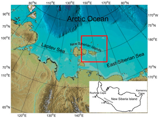
Figure 1.
Study area.
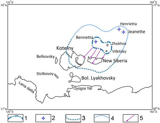
Figure 2.
Chart of glaciation of the New Siberian Islands (according to [37]): 1—the boundary of the supposed center of the Middle Neopleistocene glaciation; 2—the position of the modern glaciers; 3—the southern boundary of expansion of the Middle Neopleistocene glacier; 4—the northern boundary of the possible glacier expansion; 5—established directions of glacier movement.
3. Methods
The research was conducted using numerical mathematical modeling. It also provides for creation of a scenario of geological development of the region.
3.1. Description of the Numerical Model
To calculate the thermal state of permafrost and thermobaric conditions for gas hydrates, we use a one-dimensional model of thermal processes in bottom sediments taking into account the phase transitions between frozen and thawed ground [18,19].
Heat distribution in bottom sediments is described by solving the one-dimensional heat equation:
Ci × ∂T/∂t = (∂/∂z)(λi × ∂T/∂z),
At the boundary between frozen and thawed deposits, the condition of equality of the ground temperature to the water freezing temperature TF and Stefan condition for the moving boundary of phase transitions are allowed:
at z = ZF: λth × (∂T/∂z)th–λf × (∂T/∂z)f = L × WTot × ρD × ∂ZF/∂t,
At the upper boundary of bottom sediments corresponding to the bottom surface:
at z = 0: T = TB,
At the lower boundary of the area calculated (HS = 1500 m), the geothermal flux G is set:
at z = HS: λth × ∂T/∂z = G,
The notations used: T—ground temperature; t—time; z—depth from the bottom surface; Сi—volumetric heat capacity of the ground; λi—soil thermal conductivity coefficient; subscript i takes one of the values “f” (frozen ground) or “th” (thawed ground); WTot—relative volumetric soil moisture; L—specific heat of freezing and melting of water in the ground pores (L = 3.35 × 10⁵ J/kg); ρD—dry bulk density; TB—temperature on the bottom sediments surface; G—the geothermal flux.
Physical and thermal properties of sediments used for numerical modeling depend on the depth and composition of sediments and are set in accordance with the accepted geological model (see Section 3.2). We assume that the sediments pores are completely filled with water or ice.
The calculations of the thermal state of bottom sediments are accompanied by estimates of the thermal dynamic boundaries of the methane gas hydrates stability zone (Figure 3) [42]. The state of the GHSZ within the permafrost area strongly depends on the ground temperature and pressure, that is why the calculations were conducted with the phase curves of methane hydrate under the corresponding lithostatic pressure. In accordance with [43], the pressure in the ground layer was calculated as the hydrostatic column pressure beneath the frozen layer at the study depth and as the lithostatic pressure at the bottom of permafrost.
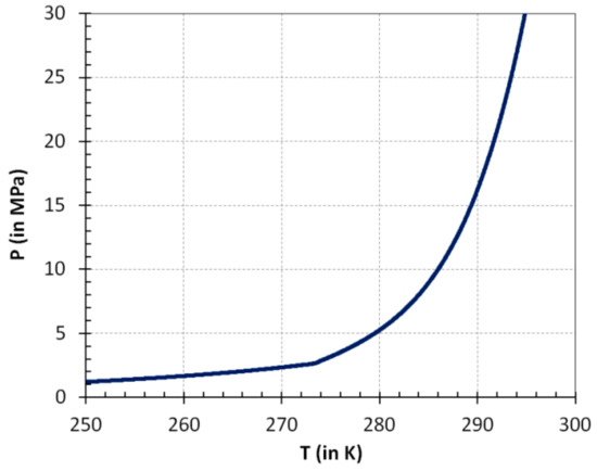
Figure 3.
Pressure–temperature equilibrium relationship in the phase diagram of the water–ice–methane–hydrate system [42].
The boundary condition on the surface of the bottom sediments (3) is determined by the transgressions–regressions periods with due account for the sea level changes, as well as by glacial conditions having existed over the last 200,000 years. Curves of temperature changes on the surface of the bottom sediments, used for modeling submarine permafrost, are shown below in Section 4.2. The geothermal flux intensity was taken equal to G = 50, 60, or 75 mW/m2, depending on the numerical calculation, which corresponds to the values of the heat flux for this region [44,45].
The numerical model implementation (1)–(4) is based on the sweep method on a discrete calculation grid with a vertical step of 0.5 m and an implicit time scheme with a step of 1 month.
3.2. Methods for Generating a Scenario of Geological Development for Research Area
The scenario of the geological development consists of a scenario of sea level fluctuations, paleogeographic (paleotemperature) scenario, and a geological model for the research area.
To set the geological structure and physical and thermophysical properties of deposits in glacial and extraglacial conditions, the data on the geological structure of the New Siberia Island were used.
The sea level scenario is built based on glacioeustatic curves of the World Ocean level fluctuations and their transformation following the regional data [11]. This approach has been applied in mathematical modeling of the evolution and the current state of the Laptev and East Siberian seas cryolithozone since 2003 [7,9]. In the present studies, we used the World Ocean level fluctuations curve and the regional data.
The eastern sector of the Russian Arctic has no paleotemperature data for several time intervals. This circumstance precludes from building a scenario of air or ground temperature dynamics using only regional data. For this purpose, to build such a scenario, the method with the isotopic paleotemperature curves obtained from the East Antarctic and Greenland glacial cores reflecting the course of global climate fluctuations, is used. Such curves are to be transformed into a regional paleotemperature scenario (model) with the help of regional paleotemperature reconstructions used as paleotemperature benchmarks. The isotopic paleotemperature curves allow for building continuous in time regional curves of the air and ground temperature dynamics using the discrete regional data [10,11]. As the latter, we used the paleotemperature reconstructions for the coastal lowlands of the north of Yakutia and the New Siberian Islands. They are created according to the width of elementary ice veins in the ice wedges [46], according to the ratio of the main rock-forming minerals [47], according to the isotopic composition of ice wedges [48,49,50], according to geothermal observations in deep boreholes [51], according to a set of paleoecological data [52,53].
Such a scenario includes a family of paleotemperature curves. We construct paletemperature curves for different isobaths and regions based on the shelf zoning in terms of bathymetry, tectonic structures, and geological development [10,11,54]. This method based on transformation of the isotope curve of Vostok station (East Antarctic), was widely used earlier [6,9,16] and is being used in a modified form now [19,23,25].
3.3. Geological Model
Assessment of the impact glaciation has on the current parameters of the permafrost and GHSZ and their evolution makes it necessary conduct such assessment under otherwise identical conditions. Therefore, to set the geological structure, sediments stratification, composition, physical and thermophysical properties of deposits in glacial and extraglacial conditions, the data on the geological structure of New Siberia Island were used. The density of the geothermal flux following the map [44], as indicated above, was 50, 60, and 75 mW/m2.
The area under research falls within the young Epikimmerian platform. Its pre-Aptian basement within this territory includes the Middle Carboniferous-Valanginian structural stage (C2-K1v). The platform cover is of Aptian-Cenozoic age (K1ap-KZ) and has the maximum thickness in depressions. Within uplifts, some horizons decrease in thickness or disappear from section [55]. New Siberian depression includes the New Siberia Island, almost the entire Faddeevsky Island, as well as the entire water area to the east of the Lyakhovsky Islands. New Siberian depression comprises terrigenous strata of the Aptian-Albian and Late Cretaceous-Cenozoic age with a thickness of up to 5 km and more. At the base of the De Long uplift, which includes the De Long Archipelago Islands, a site of the Epicarelian plate and a folded system of the Mesozoic time exist [55].
The plate cover (Late Cretaceous-Cenozoic structural floor) includes deposits of the Late Cretaceous (Bunginskaya and Derevyanogorskaya suites), Paleogene–Miocene (Anzhuyskaya suite), as well as polygenetic sediments of the Pliocene–Quaternary age [56]. The uppermost part of the section is composed of marine sediments of the Nerpichinskaya (Lower-Middle Neopleistocene) and Kanarchakskaya suites (Middle-Late Neopleistocene) [40,41].
When calculated, to ensure the lower boundary of the calculated area does not influence the permafrost bottom dynamics, it was assumed that the maximum vertically set area of the geological model should be 1.5 km. This means the properties of the deposits are to be set down to a depth of 1.5 km. According to V.K. Dorofeev et al. [56], the plate cover thickness varies from a few meters to 300 m onshore and in coastal zones to a few kilometers outside the shelf (sea depths over 500 m). The calculations take the data for two boreholes, which were subject to temperature logging and the estimation of permafrost thickness. This is borehole c-A with a depth of 200 m. It is located on the southern coast of New Siberia Island in the Derevyannye Gory tract (Figure 1 and Figure 4). Based on this borehole the Upper Cretaceous sediments thickness is more than 200 m. The deposits of the Derevyanogorskaya suite (K2dr) occurring from the surface with a thickness of 130 m are represented by tuffaceous sands, silts, brown coals with interbedded clay. The total thickness of brown coals is about 40 m. Below this suite, the Bunginskaya suite rocks (K2bn), represented by clays, mudstones, silts, and sands, were exposed by drilling. It is assumed that the section below is represented by sandstones, mudstones, silts of the Jurassic age (by analogy with the neighboring areas).
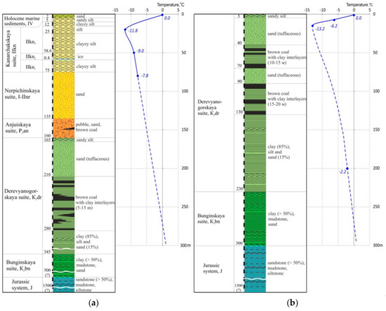
Figure 4.
The geological sections per data on boreholes c-B (a), c-A (b) (Figure 1) and the State geological map of the Russian Federation [55] and the temperature data.
In the area of Cape of Rozhin (the extreme southwestern tip of the New Siberia Island), borehole c-B (borehole depth is 80 m) penetrated modern sea sands and silts with 5 m thickness. The Kanarchakskaya suite silts with a total thickness of 70 m, at 59 m depth containing glacial ice of 40 cm thickness underlie them. Below the sands of the Nerpichinskaya suite were penetrated. Their thickness is set equal to 60 m. Below gravels and sands of the Anzhuyskaya suite are located. Deposits of the Derevnogorskaya and Bunginskaya suites underlie them. Jurassic sandstones, mudstones, and silts are represented from a depth of 500 m and more (Figure 4). The lower part of the given section is compiled based on the materials of the regional generalization [55]. The solid line of the temperature curve is plotted according to the results of geothermal observations in the borehole, the dashed line—following the geothermal gradient in the depth interval of 50–80 m.
Thermophysical characteristics (Table A1) were assigned based on the lithological composition, geological and genetic type and age of the sediments according to the data obtained within the adjacent territories [57,58,59,60] regarding the known physical characteristics of the deposits from boreholes c-A and c-B.
4. Development Scenario for the Region
4.1. Sea Level Dynamics Scenario
The scenario of sea level dynamics in extraglacial conditions. For this research (Figure 5), we took the curve of the World Ocean level fluctuations as the initial one [61]. We faced an extreme shortage of regional data and their inequality to transform this curve into the curve of the East Siberian Sea. Only the course of the Flandrian transgression in the Laptev Sea has been sufficiently completely characterized by such data [62]. Particularly, we mean the information about the dating and altitude of the points of continental sedimentation change into marine during the Flandrian transgression. To determine the shelf drainage limit within cryochron MIS-2, we used the materials of permafrost interpretation of the seismoacoustic data on the shelf edge [63].
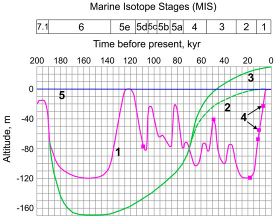
Figure 5.
Regional fluctuations of sea level (purple line 1) and glacioisostatic movements of the ground surface at the southern (dashed green line 2) and northern (solid green line 3) parts of the study area. Purple dots 4—dated sea level benchmarks [62,63,64,65,66]; blue line 5—recent sea level.
The information on the level fluctuations within MIS-3 is contradictory. Only faunistic data in the East Siberian sector of the Arctic are considered as reliable [64]. They show that the level did not exceed abs. heights of −40 m (4 in Figure 5) Contrast alternating level fluctuations during MIS-5 are provided with only one date (IR-OSL 111 ± 5 thous. years ago) [65]. It corresponds to its low state for MIS-5d within the western part of the Laptev Sea (4 in Figure 5). The history of the sea level fluctuations at the end of the Middle Neopleistocene has been also poorly characterized by the regional data. When characterizing the sea level in the last interglacial of the Middle Neopleistocene, it was taken into account that the data on the Konkovskaya transgression in the lower reaches of the river Kolyma are insufficiently substantiated in terms of age [66]. The use of the listed data made it possible to build a scenario variant (curve) for the extraglacial conditions (1 in Figure 5).
The scenario of the earth surface and sea level dynamics in the glacial area. Glacioisostatic earth crust movements accompany glaciation. During glaciation, the glacier bed sinks under glacial load. When the glacier degrades and the glacial load decreases, the bed rises. The processes in the upper mantle (asthenosphere) cause these alternating movements. It has the ability of plastic flow within a gravity field [67]. Within the glacial area, the glacioisostatic curve is considered as one of the main parameters to reconstruct the hypsometry of the glacial bed, shores, and their position relative to the sea level. It characterizes the course of glacioisostatic movements in time, that is, the progress of changes in the glacial bed and shores hypsometry [54].
For the glacioisostatic curve plotting, the main thing is reconstruction of the altitude position of the glacial bed in the pessium MIS-6. As the initial data for reconstruction we took correlation of ice sheet with the deepest part of the section of the lower subsuite of the Kanarchakskaya suite [40], as well as the sea depth (50 m) according to the malacofauna-related data [55] and the shelf drainage limits in MIS-6. As far as the East Siberian shelf is concerned, the latter were taken following the data on shelf drainage in MIS-2 [62] and already mentioned results of the permafrost interpretation of the seismoacoustic data on the edge of the Laptev Sea shelf (120 m) [5]. Based on the accepted data the abs. height of the glacial bed in MIS-6 was minus 170 m.
Figure 5 shows two glacioisostatic curves. The following data were used to plot them. Particularly, the abs. heights of the glacial bed in MIS-6 and the bottom of sediments comprising ice sheet, as well as the 14C date of mammal bone residues of the mammoth complex on the New Siberia and Faddeevsky Islands. Based on 14C data, marine sedimentation not later than 54 ka was replaced with accumulation of continental sediments of the Late Neopleistocene Ice Complex [40]. In terms of calendar time, this date corresponds to the age of at least 59,000–60,000 years ago [68]. At this time, the shelf was drained to 80–100 m isobaths (Figure 5). The beginning of the regression accrues to the time of 75–70 ka. Therefore, the islands in their current form could have been formed from 75–70 to 60 ka BP. The abs. heights of the roof of the lower subsuite of the Kanarchakskaya suite at the Cape Kamenny are 36–40 m [40]. It underlies sheet ice and was a glacier bed within MIS-6. In other places in the northern part of the islands, this stratum is located lower. Additionally, in the south the New Siberia Island goes below the sea level. The above data and modern abs. heights of the bottom of the lower Kanarchakskaya suite underlying the ice sheets provided the basis for plotting the glacioisostatic curves (2 and 3, Figure 5, for the south and north of the island, respectively). Curve 3 was selected as the main one.
According to curve 3 in Figure 5 and its relationship with the curve of the sea level fluctuations (1 in Figure 5) the glacial area comprised a sea basin in the interval of 180–70 ka. Its level correlated with the glacioisostatic curve. Under extraglacial conditions, subaerial environments were found at this time. Within the interval from 70,000 years ago to the present time according to the ratio of the indicated curves (3 and 1 in Figure 5), the glacial area, as well as the extraglacial area, were subject to the subaerial conditions. The feature of the glacial area was formation (due to glacioisostatic uplift) of a marine terrace up to 40 m high [40].
Thus, the main changes in the course of the sea level fluctuations are described by the ratio of the glacioisostatic curve and the sea level fluctuation curve under extraglacial conditions.
4.2. Paleotemperature Scenario
Setting the initial temperature conditions. The part described above shows that during the calculation period the sea conditions existed for a longer time within the glacial area rather than outside this area. The marine periods are the most important warming factor for permafrost formation. To set the initial conditions in the glacial area and outside it, the following should be kept in mind. Within the period preceding the calculated one (200,000 years ago–the present time), the continental regime prevailed in extraglacial conditions [55]. Predominance of the continental regime with cryochron temperature at the level from −23 to −27 °C (Figure 6) determines the long-term existence of submarine permafrost under the extraglacial conditions. According to the data [9], the period of continuous existence of permafrost on the shelf within 0–50 m isobaths was estimated for the last 400,000 years.
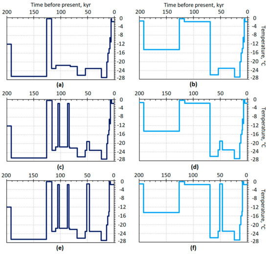
Figure 6.
Paleotemperature scenario for isobath area: (a,b) 5 m; (c,d) 20 m; (e,f) 40 m. Dark blue line—for extraglacial conditions (a,c,e); blue line—for the glacial conditions (b,d,f).
The glacial area developed differently. During accumulation of the Nerpichinskaya suite (the first half of the Middle Neopleistocene according to [40]) there was the sea. The sea having existed for hundreds of thousands of years determines lack of permafrost during this long period.
The abovesaid made it possible to set the initial values of the rock temperature equal to −1.8 within the glacial area and −12 °C outside it. The first value roughly corresponds to the current average annual temperature of the bottom water to north of the New Siberia Island, the second value corresponds to the current average annual ground temperatures of the New Siberia Island according to the geothermal observations in boreholes c-A and c-B. The set value for the extraglacial conditions is the highest of possible. It corresponds to the thermochron values. Its duration could hardly exceed 10,000 years. Thus, the initial conditions were set taking into account geological development, both in the glaciated area and outside its boundaries.
Construction of a paleotemperature scenario for the extraglacial area. The scenario allowing for setting the upper boundary conditions when modeling (Figure 6a,c,e) was established based on the methodology in [10,11]. We used the studies, which made it possible to reconstruct the temperature conditions of sedimentation on the New Siberian Islands and the coastal lowlands of northern Yakutia within the different time intervals [46,47,49,50,52,53,65].
The main initial paleodata for MIS-2 were the reconstructed sediment temperatures: −27 °С in the modern Arctic tundra at Cape Svyatoi Nos; from −22 to −26 °C in woodlands of different parts of the lowlands [47]; from −22 to −27 °C in woodlands and subarctic tundra of the lower reaches of the Kolyma [46]. The values of temperatures for warming MIS-5e from −2 to −3 °C [47] are restored for Cape Svyatoi Nos and the range from 0 to −5 °C for conditions from woodlands to arctic tundra [46]. These authors have given the same values for the early Holocene warming. Changes in air temperatures for the conditions of the southern and northern coasts of the Dm. Laptev Strait over the past 200,000 years are given in [49,50,53,65].
Construction of a paleotemperature scenario for the glacial area. The peculiarities that define the construction of the paleotemperature scenario for the glacial area are the determination of the glacier thickness and setting the ground temperature below the glacier. Glaciation, as it is known [69,70], causes glacial bed subsidence, as it is accompanied by displacement of a subcrustal substance under the glacier load. The density of the subcrustal substance is close to 3.3–3.5 g/cm3, and of ice −0.9 g/cm3 [66]. Therefore, to restore isostatic equilibrium during glaciation, the earth’s surface lowered by 2/7 of the average ice thickness. Under deglaciation, the opposite process occurs: the earth’s surface rises by the same value. Therefore, having determined the vertical movement value for the glacier bed for the period MIS-6 till present, it is possible to determine the glacier thickness.
The value of this movement is 170 and 200 m (2 and 3 in Figure 5). These values were adopted to estimate the altitude ratio between sea level and coastline. The concern arose from the question if it was possible to use them to estimate the magnitude of the postglacial uplift. In the first approximation, the authors consider it is possible. At the same time, we can also take into account the role of glacial exaration of the apex surface, composed of deposits of Kanarchakskaya suite, and incompleteness of deglaciation. The first factor mentioned can be inferred based on the sea depth in the glacial area. These are the first tens of meters. The estimation of the deglaciation incompleteness effect can add an additional 10 m. This value will result from the melting of the largest ice mass (2/7 of 35 m) on the New Siberia Island. Taking into account the abovementioned terms allows estimating the value of MIS-6 glacier bed elevation as 200–220 m, and the glacier thickness as 700–770 m. These are the maximum values. In the south of the New Siberia Island, the glacier thickness may reach 600–630 m and less. In our calculations, we assumed the glacier thickness equal to 600 m.
To estimate the below glacier ground temperature, we used the value of the geothermal gradient obtained from the geothermal observations in the borehole in the village Tiksi (2 °C/100 m [11,71]). Figure 6b,d,f shows that within cryochron MIS-6 the surface temperature under the glacier was 12 °C higher than within the extraglacial area (−14.5 instead of −26.5 °C).
The glacier is not the only warming factor in the glacial area compared to the extraglacial one. Over the period from 116,000 to 70,000 years ago, the glacial area comprised the sea, while the extraglacial area was subject to the continental conditions with the natural environment of the drained shelf. The ground temperature 20 °C lower than within the glacial area caused active shelf freezing.
5. Results of Modeling
5.1. Testing of Geological Development Scenario
Mathematical modeling at the sites provided with reliable geocryological data usually performs testing. For the glaciation area, we took the boreholes sites on the New Siberia Island (boreholes c-A and c-B) (Figure 1), provided with the geothermal data. Drilling and thermal logging were conducted during the state geological survey at a scale of 1:200,000 in the 1970s.
The geological section, required for solving Stephan’s task, in the upper 80 (borehole c-B) and 200 m (borehole c-A) was set by the drilling results, and below—following the geological survey data summarized in [55,56,72]. According to the geothermal observations in borehole c-B (located at the southwestern tip of the New Siberia Island), the average annual temperature was −11.5 °C, the temperature at the bottomhole was −7.6 °C. The permafrost thickness, calculated from the geothermal gradient is 250–255 m [71,73]. The paleotemperature curve and the results of test modeling are shown in Figure 7. Correction of rock properties allowed us to obtain correspondence between the field and estimated data.
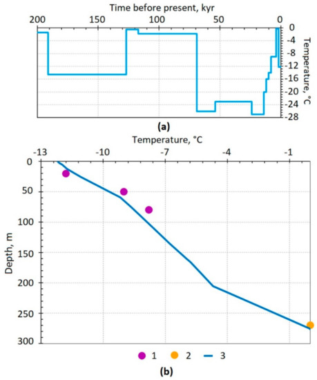
Figure 7.
Testing the scenario of the geological development based on the geocryological data of borehole c-B: (a) paleotemperature scenario; (b) results of test modeling at the heat flux of 60 mW/m2: 1—ground temperature according to the geothermal observations in borehole c-B; 2—temperature obtained by extrapolating data for the borehole with due account for the geothermal gradient; 3—estimated temperature curve.
We also conducted test modeling using the data from borehole c-B. The average annual ground temperature in the 1970s here was −13.2 °C, the bottomhole temperature −2 °C, the permafrost thickness according to thermal logging and geothermal gradient 235–240 m [71]. Test modeling also showed a coincidence of the calculated data with the field data. The calculations encouraged the conclusion that the generated paleotemperature scenario and geological model are realistic and can be used for mathematical modeling of shelf cryolithozone evolution and current state.
5.2. Permafrost Distribution and Thickness
The modeling results for the extraglacial and glacial conditions by the scenario (Figure 6) under the heat flux of 50, 60, and 75 W/m2 are shown in Figure 8 for areas of 5, 20, and 40 m isobaths. Figure 8 shows the dependence of the depth of the permafrost bottom surface (thickness) on the geothermal flux, sea depth (isobaths), and the geological development history (glacial, extraglacial conditions).
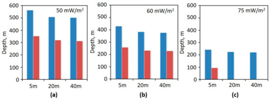
Figure 8.
Shelf permafrost under the extraglacial (blue bars) and glacial conditions (red bars) on 5, 20, and 40 m isobaths. Modeling results for the recent period with the heat flux: (a) 50 mW/m2; (b) 60 mW/m2; (c) 75 mW/m2.
The geothermal flux density determines the rate of rocks freezing during shelf drainage and, that is especially important, the rate of permafrost degradation during shelf flooding. The dependence of the permafrost thickness on the sea depth is the dependence on the duration of the period of their aggradation during drainage and degradation during shelf flooding. This period within the glacial area is much shorter than outside this area (Figure 9 and Figure 10). According to the mentioned above, the highest current permafrost thickness should be in the area of 5 m isobaths within extraglacial conditions, and the lowest one in the area of 40 m isobaths of the glacial area under increased heat flux. Indeed, within the first indicated area it is 570 m, within the second one, the relict permafrost has completely degraded.
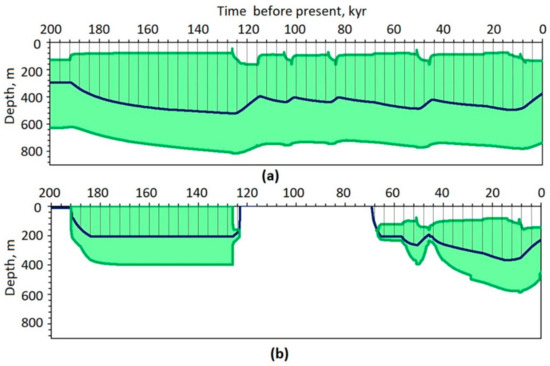
Figure 9.
Permafrost and GHSZ evolution under the extraglacial (a) and glacial conditions (b) on 40 m isobaths with the heat flux of 60 mW/m2. Permafrost—shaded area; GHSZ—green area.
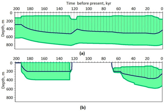
Figure 10.
Permafrost and GHSZ evolution under the extraglacial (a) and glacial conditions (b) on 5 m isobaths with the heat flux of 60 mW/m2. Permafrost—shaded area; GHSZ—green area.
For this reason, the dependence of the permafrost thickness on the value of the geothermal flux and the depth of the sea (isobaths) is reasonable to compare using the example of the extraglacial conditions, where this dependence is clearly defined. Under the extraglacial conditions, per 5, 20, 40 m isobaths, the permafrost thickness varies from 570 to 500 m at the heat flux of 50 mW/m2, from 430 to 370 m at 60 mW/m2, and from 240 to 220 m at 75 mW/m2.
The dependence of the permafrost thickness on the depth under the extraglacial conditions is much weaker. It gradually decreases as the sea depth increases from 5 to 20 and further to 40 m at each heat flux value of 50, 60, and 75 mW/m2. The reduction is expressed in values from 10 to 20–25 m.
The dependence of the permafrost thickness on its location within the glacial area or outside is expressed almost as clearly as for the heat flux. The maximum permafrost thickness is intrinsic to 5 m isobath area—about 340 m under the heat flux of 50 mW/m2, 220–230 m less than within extraglacial conditions. With this value of the heat flux at 20 and 40 m isobaths, the permafrost thickness is reduced by 200 m compared to the extraglacial conditions. At 60 mW/m2, such reduction amounts to 190 m for 5 m isobath and 170 m for 40 m isobath. At 75 mW/m2, relict frozen deposits are found only at 5 m isobath. Their thickness here is almost 100, which is 130,140 m less than within extraglacial conditions. However, on 20 and 40 m isobaths, permafrost thaws. Such a significant transformation of the permafrost strata within the glacial area at 20 and 40 m isobaths at 75 mW/m2 is stipulated by the following.
When immersed under the sea the frozen deposits are presented as ice bonded permafrost. As the degradation proceeds, along with an increase in the ground temperature, it is transformed into a stratum of plastic-frozen deposits (ice bearing permafrost), where ice is contained in the form of inclusions. Figure 8 shows the results of such degradation, namely, the gradual decrease in the content of ice bonded permafrost in the strata due to an increase in unfrozen water volume and reduction in the ice amount, at the heat flux of 50 and 60 mW/m2, both for the glacial and extraglacial conditions. The results of the same degradation, together with temperature increase, change in the unfrozen water and ice ratio, are reflected at the heat flux of 75 mW/m2 for 5 m isobath within the glacial conditions. The situation is different at 20 and 40 m isobaths within the glacial area. The degradation having sharply accelerated proves that temperature in the strata under degradation increases to the values corresponding to the freezing–thawing point of the pore water, that the phase transitions in it are minimized and that rate of permafrost thawing sharply grows. Rate growing leads to complete permafrost thawing at 20–40 m isobaths.
Thus, with the heat flux of 75 mW/m2, discontinuous or sporadic relict permafrost can occur in the glacial area, while within extraglacial conditions, continuous relict permafrost of 200–240 m thickness can occur.
5.3. Evolution of Permafrost
The modeling results show that the most significant impact the glaciation had on the evolution of the permafrost (Figure 9 and Figure 10). Under extraglacial conditions, permafrost continuously existed throughout the entire estimated period (200 kyr before present). Within the glacial area, on the contrary, there was a break. Permafrost’s existence fell within the intervals of 190–125 and from 70 to 60 ka. During the first interval they formed and existed under the glacier, the second was the interval of their subaerial existence. Its beginning is connected to the sea regression in MIS-4. The age of modern permafrost is reckoned by 60,000–70,000 years.
Permafrost formation and degradation have resulted from the climate and sea level fluctuations. Therefore, the fluctuations are evidenced in the permafrost bottom depth and thickness (Figure 9 and Figure 10). In this case, they are evidenced in a smoothed form and with a delay. Smoothness is most clearly noted at 5 m isobath (Figure 9). The lag of the MIS-5e optimum (125,000 years ago) or the MIS-2 pessium (20,000 years ago) (Figure 6), for example, both in the extraglacial and glacial conditions, is approximately 8000–9000 years. This is in good agreement with the results of other studies [9,74]. The highest permafrost thickness, as evidence of the pessiums MIS-6 and MIS-2, is 450 and 380 m, respectively, within the extraglacial conditions (Figure 6a,e). Under the glacial conditions (Figure 6b,f), on the contrary, the permafrost thickness in MIS-6, which has formed under the glacier, was lower (200 m) than in MIS-2 (360 m). Thus, the glacier impact was expressed in the reduction of the permafrost thickness by 160 m.
During the warm intervals, the permafrost thickness under the extraglacial conditions was lower. As a response to the MIS-5e optimum, it was 210 m. After the warmest interval in the MIS-3 interstadial, because of the sea level rise, it was 270 m at 40 m isobath. At 5 m isobath, warming did not show up at all, since the sea reached only the modern isobath of 40 m (Figure 6e).
5.4. Current State of Gas Hydrate Stability Zone
The GHSZ formed together with the permafrost under extraglacial and glacial conditions with heat flux from 50 to 75 mW/m2 (Figure 9 and Figure 10). The position of the upper boundary of the GHSZ slightly depends on the presence or absence of the glacier in the past. It is located inside permafrost mass a depth of 130–160 m within the extraglacial conditions and at a depth of 140–160 m in the glacial conditions (Figure 9, Figure 10 and Figure 11).
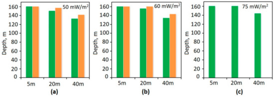
Figure 11.
The upper boundary of the GHSZ under the extraglacial (green bars) and glacial (orange bars) conditions on 5, 20, and 40 m isobaths. Modeling results for the recent period with the heat flux: (a) 50 mW/m2; (b) 60 mW/m2; (c) 75 mW/m2.
The lower boundary of the GHSZ within the glacial conditions is located at depths close to 700 m at 50 mW/m2, at 450–500 m at 60 mW/m2 (Figure 12). At 75 mW/m2, per our calculations, the hydrate stability zone has not been kept thus far. Under the extraglacial conditions, its depths are 900–1050 and 770–790 m at 50 and 60 mW/m2, respectively. At 75 mW/m2, the depths are generally close to 400 m. The deep position of the lower boundary and the high GHSZ thickness, especially on 5 m isobath at 50 mW/m2, are caused by high permafrost thickness. Accordingly, the lower permafrost thickness in the glacial area determines the shallower position of the lower boundary and the lower thickness of the GHSZ as compared to the extraglacial conditions.
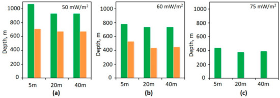
Figure 12.
The upper boundary of the GHSZ under the extraglacial (green bars) and glacial (orange bars) conditions on 5, 20, and 40 m isobaths. Modeling results for the recent period with the heat flux: (a) 50 mW/m2; (b) 60 mW/m2; (c) 75 mW/m2.
5.5. Evolution of Gas Hydrate Stability Zone
The GHSZ evolution is associated with the dynamics of the P-T conditions, i.e., with permafrost dynamics and the glaciation existence. Evolution displays itself, above all, within the periods of GHSZ existence, as well as in the dynamics of its lower and upper boundaries and thickness, caused by climate and sea level fluctuations. Under the extraglacial conditions, the GHSZ lifetime exceeded the estimated period (Figure 9a and Figure 10a). Within the glacial area, the periods of GHSZ changed on a rotating basis with the periods without GHSZ (Figure 9b and Figure 10b). The periods of existence fell on the intervals of 190–125 and from 70–60 ka with a break for the interval of 125–70 ka.
The configuration of the GHSZ lower and upper boundaries and thickness is closely related to the climate, sea level fluctuations and glacier existence. Under the extraglacial conditions, interglacials (MIS-7, 5e, 1) and short-term warm extremums, which were accompanied by the sea level rise (MIS-5c, 5a, 3), on 40 m isobaths are distinguished by depressions of the GHSZ roof up to 100–120 m (Figure 9a). On 5 m isobaths, such depressions are intrinsic only to interglacials (Figure 10a).
The response of the GHSZ lower boundary to the climate fluctuations within the extraglacial conditions repeats the relief of the permafrost lower boundary (Figure 9a and Figure 10a). However, it has a smoother form than the response of the permafrost bottom. The delay is of the same sequence as in the case of the permafrost.
Within the glacial area, two circumstances are noteworthy. The first is the formation of the GHSZ with a roof coinciding with the glacier bed (Figure 9b and Figure 10b). The glacial load causes this. The second is the relief-formed response of the roof, and especially of the GHSZ lower boundary, to the climate and sea level fluctuations on 40 m isobath (Figure 9b). This is not the case on 5 m isobath.
The information on the depth of the GHSZ lower boundary and thickness under a heat flux of 60 mW/m2 is presented in Table 1. It should be noted that the depth of the GHSZ bottom and its thickness under the extraglacial conditions is significantly more compared to the glacial conditions. Within the pessium MIS-6 they were 800 and 740 m, within the MIS-2–770, and 730 m, respectively.

Table 1.
Dynamics of the depth of the GHSZ lower boundary (numerator) and thickness (denominator) at the heat flux of 60 mW/m2.
Contrary to the results of the numerical experiment with a heat flux of 60 mW/m2, the calculation based on a flux of 75 mW/m2, shows that the gas hydrate stability zone is formed only during the oceanic regressions periods. At the same time, under the glacial conditions, the GHSZ is absent in the recent period. It was destroyed in the Holocene: 4000 years ago in the area of 5 m isobaths, 5000 years ago at 20 m isobaths, and 6000 years ago at 40 m isobaths. Since the conditions favorable for the GHSZ formation are breached, therefore, gas hydrates are possibly subject to degradation methane accumulates in the subpermafrost horizons of bottom sediments. The subsequent destruction of the permafrost layer under the effect of increased heat flux (75 mW/m2 and more) in the recent period, is likely to cause an increase of bottom deposits permeability and methane flux into the atmosphere from the shallow-water shelf.
The area of high methane emissions northward of the New Siberia Island in the research paper [23] is associated with the existence of the Great Siberian Polynya. The results of our studies indicate a possible connection of this area with permafrost degradation and GHSZ destabilization within the glaciation area of the Middle Neopleistocene with the increased heat flux.
6. Discussion and Conclusions
In the model, Romanovskii et al. [9] received the values of the permafrost thickness and the depth of the GHSZ lower boundary within the glacial area which were 1.5 times greater than in our model. The differences are explained by the fact that for this research the authors used not conditional, but real geological cross-sections. The latter contains both extended intervals of marine sedimentation, with no rocks freezing, and numerous brown coal layers with low thermal conductivity. Verification of modeling results is an issue of concern in such studies. The concern arises from the unavailability of the data required for comparison. N. Shakhova and D. Nicolsky suggest verification based on the location of the methane seeps [24]. Comparisons are often made with the permafrost thickness in nearshore boreholes [25]. However, the area of the eastern part of the Anjou Islands and the De Long archipelago does not contain such boreholes, except for those used in this study. In addition to testing the scenario and the geological model, the authors used the modeling procedure to make the results more realistic. The calculations for onshore well sites and 5, 20, and 40 m isobaths sites were carried out within a unified system. Additionally, the onshore boreholes sites are considered as benchmarks. This is a geological benchmark: well c-B and the results of generalizing the geological development of the region [55]. In addition, a geothermal benchmark in the form of temperature measurement results for the well c-B. Thus, the modeling results were constantly monitored with the geocryological data in the process of calculations that were considered as verification of the final model.
For the first time, using mathematical modeling, we studied permafrost distribution and thickness within the glaciation area at the end of the Middle Neopleistocene in the northwest of the East Siberian shelf.
It is the first time for the modeling to be based not on conventional schematized sections, but the data of drilling sediments containing, overlying, and underlying the sheet ice of the New Siberia Island. We tested the paleotemperature scenario by the results of the geothermal observations in the boreholes. This ensures the modeling results to be realistic.
The modeling results show that within the glacial area the permafrost thickness at heat flux of 50 and 60 mW/m2 is 150–200 m less than within extraglacial ones. At the heat flux of 75 mW/m2 on 20–40 m isobaths, it leads to the formation of discontinuous or sporadic permafrost.
Under the extraglacial conditions, the GHSZ formed at heat flux from 50 to 75 mW/m2. Its lower boundary is currently located at a depth of 900–1000 m at 50 mW/m2, at a depth of about 400 m at 75 mW/m2.
The permafrost and the GHSZ strata continuously exist under the extraglacial conditions, at least during the entire estimated period (200 ka-present). Within the glacial area, during the Middle Pleistocene-Holocene, they occurred and degraded. The recent permafrost strata, as well as GHSZ with the heat flux of 50 and 60 mW/m2, exist since MIS-4 (60,000–70,000 years). At the heat flux of 75 mW/m2, permafrost is retained only in the coastal area and on 5 m isobaths, and the GHSZ is currently absent.
Author Contributions
Conceptualization, A.G.; experimental methodology, A.G., E.P. and A.P.; numerical modeling, V.M.; experiments and analysis, A.G. and V.M.; writing—manuscript and editing, A.G., V.M. and E.P.; visualization, E.P., V.M. and A.P.; funding acquisition, V.M. All authors have read and agreed to the published version of the manuscript.
Funding
The research was supported by the Russian Science Foundation (grant 20-11-20112).
Conflicts of Interest
The authors declare no conflict of interest.
Appendix A
Table A1.
Physical and thermophysical properties adopted in the numerical model.
Table A1.
Physical and thermophysical properties adopted in the numerical model.
| Lithology | Lower Layer Boundary, m | Volumetric Heat Capacity, Thawed, MJ/°C·m3 | Volumetric Heat Capacity, Frozen, MJ/°C·m3 | Thermal Conductivity, W/°C·m | Thermal Conductivity, W/°C·m | Dry Soil Density, kg/m3 | Total Water Content, Unit Fractions | Soil Salinity Degree, % | Freezing Temperature, °C |
|---|---|---|---|---|---|---|---|---|---|
| Cth | Cf | λth | λf | ρD | WTot | DSal | TF | ||
| Sand | 2 | 2.65 | 2.1 | 1.74 | 2.27 | 1190 | 0.312 | 0.103 | −0.27 |
| Sandy silt | 5 | 3.12 | 2.3 | 1.1 | 1.3 | 1550 | 0.275 | 0.65 | −1.40 |
| Clayey silt | 12 | 2.68 | 2.14 | 1.58 | 1.97 | 1370 | 0.42 | 0.34 | −0.58 |
| Silt | 25 | 3.12 | 2.3 | 1.1 | 1.3 | 1500 | 0.214 | 0.4 | −1.14 |
| Clayey silt | 59 | 3.06 | 2.91 | 1.15 | 1.15 | 1550 | 0.269 | 0.6 | −1.33 |
| Clayey silt | 75 | 2.68 | 2.14 | 1.58 | 1.97 | 1370 | 0.269 | 0.34 | −0.87 |
| Sand | 135 | 1.84 | 2.28 | 2.75 | 2.95 | 1650 | 0.245 | 0.10 | −0.15 |
| Pebble, sand, brown coal | 160 | 2.72 | 1.95 | 1.82 | 1.95 | 1490 | 0.223 | 0 | 0 |
| Sandy silt | 165 | 2.8 | 2.16 | 1.4 | 1.82 | 1830 | 0.217 | 0 | −0.10 |
| Sand (tuffaceous) | 210 | 2.5 | 2.02 | 2 | 2.29 | 1610 | 0.213 | 0 | 0 |
| Brown coal with clay interlayers (15–20 m) | 280 | 3.42 | 2.71 | 1.3 | 1.3 | 1550 | 0.216 | 0 | 0 |
| Clay (85%), silt, and sand (15%) | 345 | 2.96 | 2.38 | 1.57 | 1.8 | 1800 | 0.229 | 0 | −0.2 |
| Clay (>50%), mudstone, sand | 500 | 2.9 | 2.15 | 1.36 | 2.11 | 1820 | 0.18 | 0 | −0.2 |
| Sandstone (>50%), mudstone, siltstone | 1500 | 2.15 | 2.1 | 2.33 | 2.76 | 2670 | 0.0151 | 0 | 0 |
References
- Fartyshev, A.I. Features of Offshore Permafrost on the Laptev Sea shelf; Nauka: Novosibirsk, Russia, 1993; p. 136. [Google Scholar]
- Yakovlev, D.V.; Yakovlev, A.G.; Valyasina, O.A. Permafrost study in the northern margin of the Siberian platform based on regional geoelectrical survey data. J. Earth’s Cryosph. 2018, 12, 67–84. [Google Scholar] [CrossRef]
- Molochushkin, E.N. Thermal regime of rocks in the southeastern part of the Laptev Sea. Ph.D. Thesis, Moscow State University, Moscow, Russia, 1970. [Google Scholar]
- Gavrilov, A.V.; Romanovskii, N.N.; Romanovsky, V.E.; Hubberten, H.-W. Offshore Permafrost Distribution and Thickness in the Eastern Region of Russian Arctic. In Changes in the Atmosphere-Land-Sea System in the Amerasian Arctic. Proc. of the Arctic Regional Center; Dalnauka Publisher: Vladivostok, Russia, 2001; Volume 3, pp. 209–218. [Google Scholar]
- Romanovskii, N.N.; Gavrilov, A.V.; Kholodov, A.L.; Pustovoit, G.P.; Hubberten, H.-W.; Kassens, H.; Niesen, F. The Forecasting Map of Laptev Sea Shelf Off-shore Permafrost. Permafrost. In Proceedings of the Seventh International Conference, Yellowknife, NT, Canada, 23–27 June 1998; pp. 967–972. [Google Scholar]
- Romanovskii, N.N.; Kholodov, A.L.; Gavrilov, A.V.; Tumskoy, V.E.; Hubberten, H.-W.; Kassens, H. Ice-Bonded Permafrost Thickness in the Eastern Part of the Laptev Sea Shelf (Results of Computer Modeling). J. Earth’s Cryosph. 1999, 3, 22–32. [Google Scholar]
- Romanovskii, N.N.; Hubberten, H.-W.; Gavrilov, A.V.; Tumskoy, V.E.; Kholodov, A.L. Permafrost of the East Siberian shelf and coastal lowlands. Quat. Sci. Rev. 2004, 23, 1359–1369. [Google Scholar] [CrossRef]
- Romanovskii, N.N.; Hubberten, H.-W.; Gavrilov, A.V.; Eliseeva, A.A.; Tipenko, G.S. Offshore permafrost and gas hydrate stability zone on the shelf of East Siberian Seas. Geo-Mar. Lett. 2005, 25, 167–182. [Google Scholar] [CrossRef]
- Delisle, G. Temporal variability of subsea permafrost and gas hydrate occurrences as function of climate change in the Laptrv Sea, Siberia. Polarforschung 2000, 68, 221–225. [Google Scholar]
- Gavrilov, A.V.; Tumskoy, V.E. Model of mean annual temperature history for the Yakutian coastal lowlands and Arctic shelf during the last 400 thousand years. Permafrost. In Proceedings of the Eighth International Conference on Permafrost, Zurich, Switzerland, 21–25 July 2003; Volume 1, pp. 287–290. [Google Scholar]
- Gavrilov, A.V. Cryolithozone of the East Siberian Arctic shelf (Current State and History of Development in the Middle Pleistocene—Holocene). Available online: https://istina.msu.ru/dissertations/2826455/ (accessed on 27 October 2020).
- Romanovskii, N.N.; Hubberten, H.-W.; Gavrilov, A.V.; Tumskoy, V.E.; Tipenko, G.S.; Grigoriev, M.N.; Siegert, C. Thermokarst and Land-Ocean Interactions, Laptev Sea region, Russia. Permafr. Periglac. Process 2000, 11, 137–152. [Google Scholar] [CrossRef]
- Tumskoy, V.E. Thermokarst and Its Role in the Development of the Laptev Sea Region During the Late Pleistocene and Holocene. Ph.D. Thesis, Moscow State University, Moscow, Russia, 2002; p. 26. [Google Scholar]
- Gavrilov, A.V.; Romanovskii, N.N.; Hubberten, H.-W. Paleogeographic scenario of the postglacial transgression on the Laptev Sea shelf. J. Earth’s Cryosph. 2006, 10, 39–50. [Google Scholar]
- Romanovskii, N.N.; Hubberten, H.-W.; Gavrilov, A.V.; Eliseeva, A.A.; Tipenko, G.S.; Kholodov, A.L.; Romanovsky, V.E. Permafrost and Gas Hydrate Stability Zone evolution on the Eastern Part of the Eurasia Arctic Sea Shelf in the Middle Pleistocene-Holocene. J. Earth’s Cryosph. 2003, 7, 51–64. [Google Scholar]
- Romanovskii, N.N.; Eliseeva, A.A.; Gavrilov, A.V.; Tipenko, G.S.; Hubberten, H.-W. Evolution and Current State of Frozen Strata and Zones of Stability of Gas Hydrates in the Rifts of the East Arctic Shelf. System of the Laptev Sea and Adjacent Arctic Seas. In Current State and History of Development; MSU: Moscow, Russia, 2009; pp. 292–319. [Google Scholar]
- Malakhova, V.V.; Golubeva, E.N. Modeling of the dynamics subsea permafrost in the East Siberian Arctic Shelf under past and future climate change. In Proceedings of the 20th International Symposium on Atmospheric and Ocean Optics: Atmospheric Physics, Novosibirsk, Russia, 23–27 June 2014; p. 92924D. [Google Scholar] [CrossRef]
- Malakhova, V.V. Estimation of the subsea permafrost thickness in the Arctic Shelf. In Proceedings of the 24th International Symposium on Atmospheric and Ocean Optics: Atmospheric Physics, Tomsk, Russia, 2–5 July 2018; p. 108337T. [Google Scholar] [CrossRef]
- Malakhova, V.V.; Eliseev, A.V. Uncertainty in temperature and sea level datasets for the Pleistocene glacial cycles: Implications for thermal state of the subsea sediments. Glob. Planet. Chang. 2020, 192, 103249. [Google Scholar] [CrossRef]
- Shakhova, N.; Semiletov, I.; Leifer, I.; Salyuk, A.; Rekant, P.; Kosmach, D. Geochemical and geophysical evidence of methane release over the East Siberian Shelf. J. Geophys. Res. 2010, 115, C08007. [Google Scholar] [CrossRef]
- Shakhova, N.; Semiletov, I.; Romanovsky, V.; Pipko, I. Methan Climate Forcing and Methane Observation in the Siberian Arctic Land-Shelf System. World Resour. Rev. 2004, 16, 503–541. [Google Scholar]
- Shakhova, N.; Semiletov, I. Methane release and coastal environment in the East Siberian Arctic shelf. J. Mar. Syst. 2007, 66, 227–243. [Google Scholar] [CrossRef]
- Dmitrenko, I.; Kirillov, S.; Tremblay, L.; Kassens, H.; Anisimov, O.; Lavrov, S.; Razumov, S.; Grigoriev, M. Recent changes in shelf hydrography in the Siberian Arctic: Potential for subsea permafrost instability. J. Geophys. Res. Oceans 2011, 116, C10027. [Google Scholar] [CrossRef]
- Shakhova, N.; Semiletov, I.; Leifer, I.; Sergienko, V.; Salyuk, A.; Kosmach, D.; Chernikh, D.; Stubbs, C.; Nicolsky, D.; Tumskoy, V.; et al. Ebullition and storm-induced methane release from the East Siberian Arctic Shelf. Nat. Geosci. 2014, 7, 64–70. [Google Scholar] [CrossRef]
- Nicolsky, D.; Shakhova, N. Modeling subsea permafrost in the East Siberian Arctic Shelf: The Dmitry Laptev Strait. Environ. Res. Lett. 2010, 5, 015006. [Google Scholar] [CrossRef]
- Nicolsky, D.J.; Romanovsky, V.E.; Romanovskii, N.N.; Kholodov, A.L.; Shakhova, N.T.; Semiletov, I.P. Modeling sub-sea permafrost in the East Siberian Arctic Shelf: The Laptev Sea region. J. Geophys. Res. Earth Surface 2012, 117. [Google Scholar] [CrossRef]
- Malakhova, V.V.; Eliseev, A.V. Influence of rift zones and thermokarst lakes on the formation of subaqueous permafrost and the stability zone of methane hydrates of the Laptev sea shelf in the Pleistocene. Ice Snow 2018, 58, 231–242. [Google Scholar] [CrossRef]
- Anisimov, O.A.; Borzenkova, I.I.; Lavrov, S.A.; Strel’chenko, Y.G. The current dynamics of the submarine permafrost and methane emissions on the shelf of the Eastern Arctic seas. Ice Snow 2012, 52, 97–105. [Google Scholar] [CrossRef]
- Kuzin, V.I.; Platov, G.A.; Golubeva, E.N.; Malakhova, V.V. Certain Results of Numerical Simulation of Processes in the Arctic Ocean. Izv. Atmos. Ocean. Phys. 2012, 48, 102–119. [Google Scholar] [CrossRef]
- Afanasenko, V.E.; Buldovich, S.N.; Romanovskii, N.N. On the manifestation of mineral waters in the northern part of the Kular ridge. Bull. Mos. Society Nat. Inv. 1973, 48, 91–102. [Google Scholar]
- GRID-Arendal. Available online: https://www.grida.no/resources/13519 (accessed on 27 October 2020).
- Overduin, P.P.; Schneider von Deimling, T.; Miesner, F.; Grigoriev, M.N.; Ruppel, C.; Vasiliev, A.A.; Lantuit, A.H.; Juhls, B.; Westermann, S. Submarine Permafrost Map in the Arctic Modeled Using 1-D Transient Heat Flux (SuPerMAP). J. Geophys. Res. Oceans 2019, 124, 3490–3507. [Google Scholar] [CrossRef]
- Razumov, S.O.; Spektor, V.B.; Grigoriev, M.N. A Model of the Late-Cenozoic Cryolithozone Evolution for the Western Laptev Sea Shelf. Okeanologiya 2014, 54, 679–693. [Google Scholar] [CrossRef]
- Arzhanov, M.M.; Malakhova, V.V.; Mokhov, I.I. Modeling thermal regime and evolution of the methane hydrate stability zone of the Yamal peninsula permafrost. Permafr. Periglac Process 2020, 31, 487–496. [Google Scholar] [CrossRef]
- Anisimov, M.A.; Tumskoy, V.E. The subsurface sheet ice of the New Siberia Island (Novosibirskie Islands, Russia). In Earth Cryosphere as a Life Support Environment; Pushchino, Russia, 2003; pp. 232–233. [Google Scholar]
- Anisimov, M.A.; Tumskoy, V.E.; Ivanova, V.V. The subsurface ice at Novosibirskie Islands as a relic of ancient glaciation. Mater. Glaciol. Res. 2006, 101, 143–145. [Google Scholar]
- Basilyan, A.E.; Nikolsky, P.A.; Anisimov, M.A. Pleistocene glaciation of the New Siberian Islands—No more doubts. IPY News 2007/08 2008, 12, 7–9. [Google Scholar]
- Golionko, B.G.; Basilyan, A.E.; Nikolsky, P.A.; Kostyleva, V.V.; Malyshev, N.A.; Verzhbitsky, V.E.; Obmetko, V.V.; Borodulin, A.A. Fold-thrust deformations of the isl. New Siberia (Novosibirsky islands, Russia): Age, morphology and genesis of structures. Geotektonika 2019, 6, 46–64. [Google Scholar] [CrossRef]
- Tumskoy, V.E. Peculiarities of cryolithogenesis in Northern Yakutia (Middle Neopleistocene to Holocene). J. Earth’s Cryosph. 2012, 16, 12–21. [Google Scholar]
- Basilyan, A.E.; Nikolsky, P.A. Reference section of Quaternary deposits of Cape Kamenny (New Siberia). Bull. Commiss. Study Quat. 2007, 67, 76–84. [Google Scholar]
- Basilyan, A.E.; Nikolskiy, P.A.; Maksimov, F.E.; Kuznetsov, V.Y. Age of cover glaciation of the New Siberian Islands based on 230Th/U-dating of mollusk shells. In The Structure and History of the Development of the Lithosphere; Paulsen: Moscow, Russia, 2010; pp. 506–514. [Google Scholar]
- Moridis, G.J. Numerical Studies of Gas Production from Methane Hydrates. SPE J. 2003, 32, 359–370. [Google Scholar] [CrossRef]
- Tinivella, U.; Giustiniani, M.; Marin-Moreno, H. A Quick-Look Method for Initial Evaluation of Gas Hydrate Stability below Subaqueous Permafrost. Geosciences 2019, 9, 329. [Google Scholar] [CrossRef]
- Davies, J.H. Global map of Solid Earth surface heat flow. Geochem. Geophys. Geosyst. 2013, 14, 4608–4622. [Google Scholar] [CrossRef]
- Pollack, H.N.; Hurter, S.J.; Johnson, J.R. Heat flow from the Earth’s interior: Analysis of the global data set. Rev. Geophys. 1993, 31, 267–280. [Google Scholar] [CrossRef]
- Kaplina, T.N.; Kuznetsova, I.L. Geotemperature and climatic model of the sediment accumulation epoch of the Yedomnaya Suite of the Primorskaya Lowland of Yakutia. In Problems of Paleogeography of Loess and Periglacial Regions; Institute of Geography, USSR Academy of Sciences: Moscow, Russia, 1975; pp. 170–174. [Google Scholar]
- Konishchev, V.N. The cryolithogenic method for estimating paleotemperature conditions during formation of Ice Complex and subaerial periglacial sediments. J. Earth’s Cryosph. 1997, 1, 23–28. [Google Scholar]
- Vasilchuk, Y.K.; Kotlyakov, V.M. Principles of Isotope Geocryology and Glaciology; Moscow State University: Moscow, Russia, 2000; p. 616. ISBN 5-211-02557-1. [Google Scholar]
- Opel, T.; Wetterich, S.; Meyer, H.; Dereviagin, A.Y.; Fuchs, M.C.; Schirrmeister, L. Ground-ice stable isotopes at the Oyogos Yar Coast (Dmitry Laptev Strait)—Indications for Late. Clim. Past 2017, 13, 587–611. [Google Scholar] [CrossRef]
- Meyer, H.; Opel, T.; Laepple, T.; Dereviagin, A.Y.; Werner, M.; Hoffmann, K. Long-term winter warming trend in the Siberian Arctic during the mid to late Holocene. J. Nat. Geosci. 2015, 8, 122–125. [Google Scholar] [CrossRef]
- Balobayev, V.T. On the Reconstruction of Paleotemperatures of Frozen Rocks. In Development of the Cryolithozone in the Upper Cenozoic; Nauka: Moscow, Russia, 1985; pp. 129–136. [Google Scholar]
- Sher, A.V.; Kuzmina, S.A.; Kuznetsova, T.V.; Sulerzhitsky, L.D. New insights into the Weichselian environment and climate of the East Siberian Arctic, derived from fossil insects, plaints, and mammals. J. Quat. Sci. Rev. 2005, 24, 533–569. [Google Scholar] [CrossRef]
- Andreev, A.; Schirrmeister, L.; Tarasov, P.E.; Ganopolski, A.; Brovkin, V.; Siegert, C.; Hubberten, H.-W. Vegetation and climate history in the Laptev Sea region (arctic Siberia) during Late Quaternary inferred from pollen records. J. Quat. Sci. Rev. 2011, 30, 2182–2199. [Google Scholar] [CrossRef]
- Gavrilov, A.; Pavlov, V.; Fridenberg, A.; Boldyrev, M.; Khilimonyuk, V.; Pizhankova, E.; Buldovich, S.; Kosevich, N.; Alyautdinov, A.; Ogienko, M.; et al. The current state and 125 kyr history of permafrost in the Kara Sea shelf: Modeling constraints. Cryosphere 2020, 14, 1857–1873. [Google Scholar] [CrossRef]
- State geological map of the Russian Federation. Scale 1: 1,000,000 (new series). In S-53-55—New Siberian Islands. Explanatory Note; VSEGEI: St. Petersburg, Russia, 1999; p. 208. [Google Scholar]
- Dorofeev, V.K.; Blagoveshchensky, M.G.; Smirnov, A.N.; Ushakov, V.I. New Siberian Islands. In Geological Structure and Minerageny; Ushakov, V.I., Ed.; SPb., VNIIOkeanologiya: St. Petersburg, Russia, 1999; p. 130. [Google Scholar]
- Chuvilin, E.M.; Bukhanov, B.A.; Tumskoy, V.E.; Shakhova, N.E.; Dudarev, O.V.; Semiletov, I.P. Thermal conductivity of bottom sediments in the region of Buor-Khaya Bay (shelf of the Laptev Sea). Earth’s Cryosph. 2013, 17, 32–40. [Google Scholar]
- Samoilik, V.G. Physicochemical Properties of Fossil Fuels and Methods of Their Study: Textbook for Universities; Donetsk National Technical University: Donetsk, Germany, 2017; p. 193. [Google Scholar]
- Gavril’ev, R.G. Catalog of Thermophysical Properties of Rocks in the North-East of Russia; Melnikov Institute of Permafrost SB RAS: Yakutsk, Russia, 2013; p. 172. ISBN 978-5-93254-124-1 300. (In Russian) [Google Scholar]
- Thermophysical Properties of Rocks; Ershov, E.D., Ed.; Moscow State University: Moscow, Russia, 1984; p. 203. [Google Scholar]
- Rohling, E.J.; Grant, K.; Bolshaw, M.; Roberts, A.P.; Siddall, M.; Hemleben, C. and Kucera, M. Antarctic temperature and global sea-level closely coupled over the past five glacial cycles. Nat. Geosci. 2009, 2, 500–504. [Google Scholar] [CrossRef]
- Bauchab, H.A.; Mueller-Lupp, T.; Taldenkovac, E.; Spielhagena, R.F.; Kassensa, H.; Grootesd, P.M.; Thiedeb, J.; Heinemeiere, J.; Petryashovf, V.V. Chronology of the Holocene Transgression at the Northern Siberia margin. Glob. Planet. Chang. 2001, 31, 125–139. [Google Scholar] [CrossRef]
- Romanovskii, N.N.; Gavrilov, A.V.; Pustovoit, G.P.; Kholodov, A.L.; Kassens, H.; Hubberten, H.-W.; Nissen, F. Off-shore permafrost distribution on the Laptev Sea shelf. Earth’s Cryosph. 1997, 1, 9–18. [Google Scholar]
- Kovalenko, F.Y.; Kuptsova, I.A. Cenozoic marine sediments of the East Siberian Sea. In Proceedings of the XIV Pacific Scientific Congress, Khabarovsk, Russia, 20 August–1 September 1979; pp. 64–66. [Google Scholar]
- Winterfeld, M.; Schirrmeister, L.; Grigoriev, M.N.; Kunitsky, V.V.; Andreev, A.; Murray, A.; Overduin, P.P. Coastal permafrost landscape development since the Late Pleistocene in the Western Laptev Sea. Sib. Boreas 2011, 40, 697–713. [Google Scholar] [CrossRef]
- State Geological Map of the Russian Federation. Scale 1:1,000,000 (New Series). R(55)-57—Nizhnekolymsk, Explanatory Note; VSEGEI: St. Petersburg, Russia, 2000; p. 16. [Google Scholar]
- Ushakov, S.A.; Krass, M.S. Gravity and Questions of the Mechanics of the Earth’s Interior; Nedra: Moscow, Russia, 1972; p. 157. [Google Scholar]
- Reimer, P.J.; Bard, E.; Bayliss, A.; Beck, J.W.; Blackwell, P.G.; Ramsey, C.B.; Buck, C.E.; Cheng, H.; Edwards, R.L.; Friedrich, M.; et al. IntCal13 and Marine13 radiocarbon age calibration curves 0–50,000 years cal BP. Radiocarbon 2013, 55, 1869–1887. [Google Scholar] [CrossRef]
- Gutenberg, B. Changes in sea level, postglacial uplift, and mobility of the Earth’s interior. Geol. Soc. Amer. Bull. 1941, 52, 721–772. [Google Scholar] [CrossRef]
- Bylinsky, E.N. Causes of Pleistocene marine transgressions in the north of Eurasia. Bul. Com. Study Quat. 1980, 50, 35–57. [Google Scholar]
- Zaitsev, V.A. Yano-Kolyma Region. Geocryology of the USSR. Eastern Siberia and the Far East; Nedra: Moscow, Russia, 1989; pp. 240–279. [Google Scholar]
- Kos’ko, M.K.; Sobolev, N.N.; Korago, E.A.; Proskurnin, V.F.; Stolbov, N.M. Geology of Novosibirskian islands—A basis for interpretation of geophysical data on the eastern Arctic shelf of Russia. Neftegasovaà Geol. Teor. Pract. 2013, 8. [Google Scholar] [CrossRef]
- Solov’ev, V.A.; Ginsburg, G.D.; Telepnev, E.V.; Mikhalyuk, Y.N. Cryogeothermy and Natural Gas Hydrates in the Bowels of the Arctic Ocean; Sevmorgeologiya: Leningrad, Russia, 1987; p. 151. [Google Scholar]
- Malakhova, V.V.; Eliseev, A.V. The role of heat transfer time scale in the evolution of the subsea permafrost and associated methane hydrates stability zone during glacial cycles. Glob. Planet. Chang. 2017, 157, 18–25. [Google Scholar] [CrossRef]


Publisher’s Note: MDPI stays neutral with regard to jurisdictional claims in published maps and institutional affiliations. |
© 2020 by the authors. Licensee MDPI, Basel, Switzerland. This article is an open access article distributed under the terms and conditions of the Creative Commons Attribution (CC BY) license (http://creativecommons.org/licenses/by/4.0/).