
Bird Beta Diversity in Sharp Contrasting Altai Landscapes: Locality Connectivity Is the Influential Factor on Community Composition

 , ,
, ,
Abstract
:Simple Summary
Abstract
1. Introduction
2. Methods
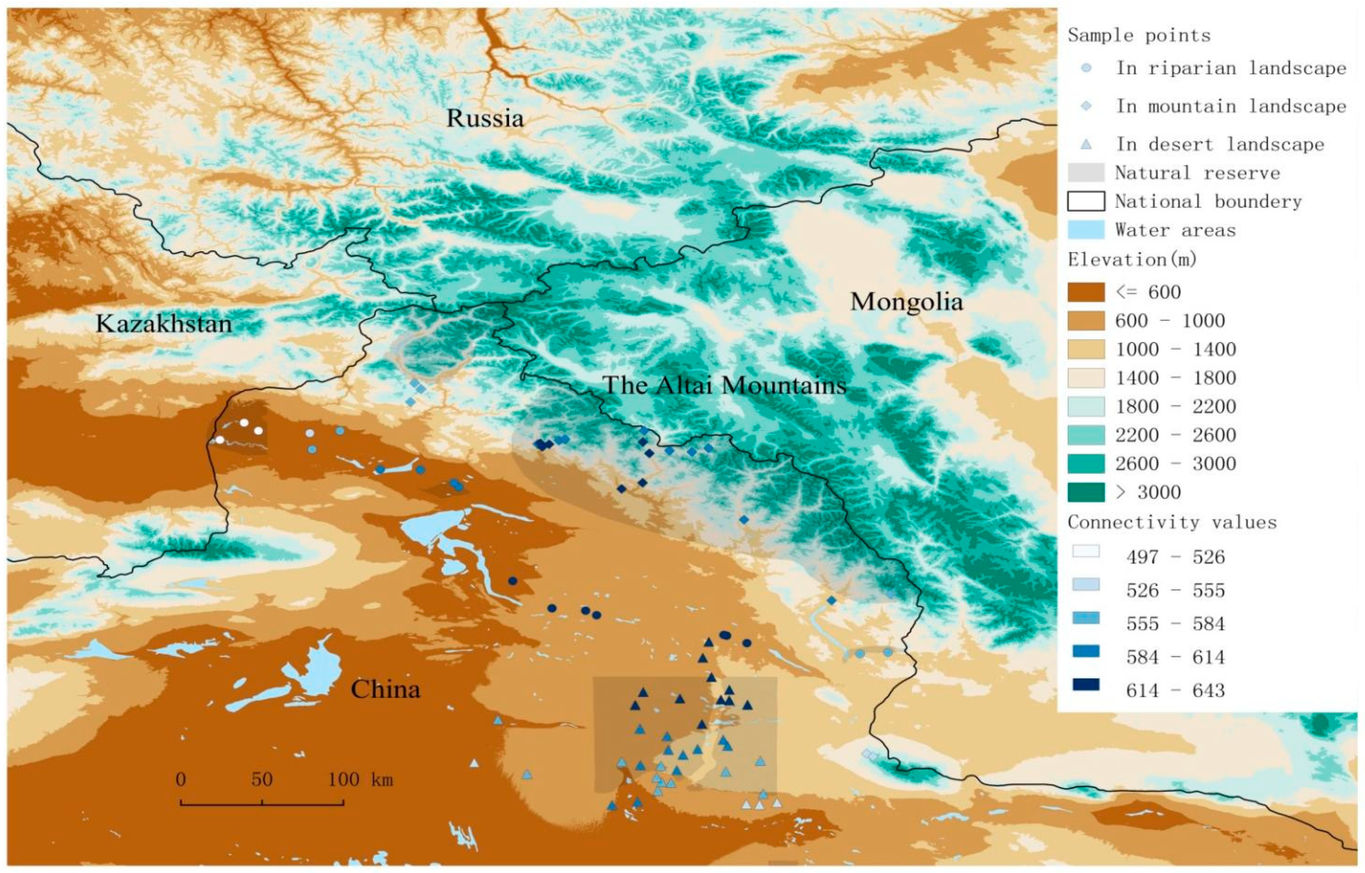
2.1. Study Area
2.2. Bird Surveys
2.3. Environmental and Spatial Variables Collection
2.4. Data Summary
2.5. Beta Diversity
2.6. Spatial, Environmental and Connectivity Predictors and Variation Partitioning
3. Results
3.1. Bird Species Richness and Beta Diversity
3.2. Spatial Structure of the Environment Variables
3.3. Contribution of Environment, Spatial Variation and Locality Connectivity to Bird Species Composition Variation
4. Discussions
4.1. Bird Species Beta Diversity
4.2. Contribution of Environment, Spatial Variation and Locality Connectivity to Bird Species Variation
5. Conclusions
Author Contributions
Funding
Institutional Review Board Statement
Informed Consent Statement
Data Availability Statement
Acknowledgments
Conflicts of Interest
Appendix A

| Detected Number | |||||
|---|---|---|---|---|---|
| Common Name | Species Name | Riparian | Mountain | Desert | Total |
| Common Starling | Sturnus vulgaris | 1572 | 0 | 1 | 1573 |
| Eurasian Tree Sparrow | Passer montanus | 1275 | 13 | 10 | 1298 |
| Black-eared Kite | Milvus lineatus | 316 | 207 | 5 | 528 |
| Rook | Corvus frugilegus | 306 | 0 | 0 | 306 |
| Carrion Crow | Corvus corone | 265 | 337 | 3 | 605 |
| European Bee-eater | Merops apiaster | 159 | 0 | 0 | 159 |
| Rufous-tailed Shrike | Lanius phoenicuroides | 141 | 8 | 45 | 194 |
| Azure Tit | Cyanistes cyanus | 122 | 0 | 0 | 122 |
| Rock Pigeon | Columba livia | 119 | 14 | 1 | 134 |
| Great Tit | Parus major | 115 | 59 | 0 | 174 |
| Eurasian Jackdaw | Corvus monedula | 108 | 0 | 0 | 108 |
| European Roller | Coracias garrulus | 87 | 0 | 0 | 87 |
| Eurasian Collared Dove | Streptopelia decaocto | 71 | 3 | 0 | 74 |
| Black-billed Magpie | Pica pica | 66 | 0 | 0 | 66 |
| European Turtle Dove | Streptopelia turtur | 64 | 0 | 0 | 64 |
| Common Hoopoe | Upupa epops | 58 | 0 | 6 | 64 |
| White Wagtail | Motacilla alba | 52 | 81 | 16 | 149 |
| Isabelline Wheatear | Oenanthe isabellina | 51 | 12 | 68 | 131 |
| Common Kestrel | Falco tinnunculus | 50 | 14 | 10 | 74 |
| European Goldfinch | Carduelis carduelis | 45 | 100 | 0 | 145 |
| Spotted Flycatcher | Muscicapa striata | 41 | 118 | 0 | 159 |
| House Sparrow | Passer domesticus | 40 | 11 | 0 | 51 |
| Grey Wagtail | Motacilla cinerea | 36 | 101 | 11 | 148 |
| Common Nightingale | Luscinia megarhynchos | 30 | 2 | 0 | 32 |
| Bearded Parrotbill | Panurus biarmicus | 29 | 0 | 0 | 29 |
| Sand Martin | Riparia riparia | 28 | 5 | 0 | 33 |
| Lesser Kestrel | Falco naumanni | 27 | 1 | 3 | 31 |
| Great Grey Shrike | Lanius excubitor | 25 | 1 | 9 | 35 |
| Common Chiffchaff | Phylloscopus collybita tristis | 21 | 7 | 0 | 28 |
| Arctic Warbler | Phylloscopus borealis | 20 | 0 | 0 | 20 |
| Fork-tailed swift | Apus pacificus | 18 | 67 | 0 | 85 |
| Chaffinch | Fringilla coelebs | 17 | 48 | 0 | 65 |
| Rufous-tailed Shrike | Lanius isabellinus | 17 | 16 | 39 | 72 |
| Desert Wheatear | Oenanthe deserti | 16 | 1 | 30 | 47 |
| Large-billed Crow | Corvus macrorhynchos | 15 | 1 | 0 | 16 |
| Coal Tit | Periparus ater | 14 | 7 | 0 | 21 |
| Greenish Warbler | Phylloscopus trochiloides | 13 | 23 | 0 | 36 |
| Eurasian Cuckoo | Cuculus canorus | 12 | 3 | 0 | 15 |
| White-backed woodpecker | Dendrocopos leucotos | 12 | 2 | 0 | 14 |
| Eurasian Hobby | Falco subbuteo | 11 | 1 | 1 | 13 |
| Blyth’s Reed Warbler | Acrocephalus dumetorum | 11 | 0 | 0 | 11 |
| Lesser Grey Shrike | Lanius minor | 11 | 0 | 0 | 11 |
| Pied Wheatear | Oenanthe pleschanka | 10 | 5 | 3 | 18 |
| Grey-headed Woodpecker | Picus canus | 10 | 5 | 0 | 15 |
| Hodgson’s Bushchat | Saxicola insignis | 10 | 0 | 0 | 10 |
| Mongolian Finch | Rhodopechys mongolica | 8 | 0 | 452 | 460 |
| Eurasian Sparrowhawk | Accipiter nisus | 7 | 6 | 0 | 13 |
| Greater Shor-toed Lark | Calandrella cinerea longipenuis | 7 | 0 | 191 | 198 |
| Richard’s Pipit | Anthus richardi | 7 | 0 | 2 | 9 |
| Pallas’s Sandgrouse | Syrrhaptes paradoxus | 6 | 0 | 348 | 354 |
| Hill Pigeon | Columba rupestris | 5 | 7 | 0 | 12 |
| Lesser Spotted Woodpecker | Dryobates minor | 5 | 1 | 0 | 6 |
| Little Owl | Athene noctua | 5 | 0 | 5 | 10 |
| Eurasian Nightjar | Caprimulgus europaeus | 5 | 0 | 1 | 6 |
| Black-bellied Sandgrouse | Pterocles orientalis | 5 | 0 | 0 | 5 |
| Daurian Partridge | Perdix dauurica | 4 | 1 | 0 | 5 |
| Barred Warbler | Sylvia nisoria | 4 | 0 | 0 | 4 |
| Hume’s Warbler | Phylloscopus humei | 3 | 103 | 0 | 106 |
| Willow Tit | Poecile montanus | 3 | 84 | 0 | 87 |
| Common Rosefinch | Erythrina erythrina | 3 | 44 | 0 | 47 |
| Common Swift | Apus apus | 3 | 18 | 90 | 111 |
| Lesser Whitethroat | Curruca curruca | 3 | 2 | 1 | 6 |
| White-crowned Penduline Tit | Remiz coronatus | 3 | 1 | 0 | 4 |
| Hen Harrier | Circus cyaneus | 3 | 0 | 0 | 3 |
| Little Bittern | Ixobrychus minutus | 3 | 0 | 0 | 3 |
| Northern Wheatear | Oenanthe oenanthe | 2 | 55 | 1 | 58 |
| Red-backed Shrike | Lanius collurio | 2 | 27 | 0 | 29 |
| Black Redstart | Phoenicurus ochruros | 2 | 13 | 0 | 15 |
| Pallid Harrier | Circus macrourus | 2 | 0 | 1 | 3 |
| Black Woodpecker | Dryocopus martius | 2 | 0 | 0 | 2 |
| Yellow Wagtail | Motacilla flava | 2 | 0 | 0 | 2 |
| Bluethroat | Luscinia svecicus | 2 | 0 | 0 | 2 |
| Northern House Martin | Delichon urbicum | 2 | 0 | 0 | 2 |
| Tawny Pipit | Anthus campestris | 2 | 0 | 0 | 2 |
| Common Kingfisher | Alcedo atthis | 2 | 0 | 0 | 2 |
| Olive-backed Pipit | Anthus hodgsoni | 2 | 0 | 0 | 2 |
| Rufous-tailed Rock Thrush | Monticola saxatilis | 1 | 31 | 1 | 33 |
| Common Stonechat | Saxicola torquata | 1 | 25 | 1 | 27 |
| Upland Buzzard | Buteo hemilasius | 1 | 16 | 7 | 24 |
| Eurasian Skylark | Alauda arvensis | 1 | 15 | 52 | 68 |
| Oriental Turtle Dove | Streptopelia orientalis | 1 | 12 | 0 | 13 |
| Dusky Thrush | Turdus eunomus | 1 | 2 | 0 | 3 |
| Eurasian Blackbird | Turdus merula | 1 | 2 | 0 | 3 |
| White-Throated Dipper | Cinclus cinclus | 1 | 1 | 0 | 2 |
| Steppe Eagle | Aquila nipalensis | 1 | 0 | 5 | 6 |
| Black-throated Accentor | Prunella atrogularis | 1 | 0 | 3 | 4 |
| Meadow Pipit | Anthus pratensis | 1 | 0 | 2 | 3 |
| Desert Warbler | Curruca nana | 1 | 0 | 1 | 2 |
| Pallas’s leaf Warbler | Abrornis proregulus | 1 | 0 | 0 | 1 |
| Eurasian Bullfinch | pyrrhula griseiventris | 1 | 0 | 0 | 1 |
| Eurasian Golden Oriole | Oriolus oriolus | 1 | 0 | 0 | 1 |
| European Greenfinch | Chloris chloris | 1 | 0 | 0 | 1 |
| Desert Lesser Whitethroat | Sylvia minula | 1 | 0 | 0 | 1 |
| Marsh Tit | Poecile palustris | 1 | 0 | 0 | 1 |
| Greater Spotted Eagle | Clanga clanga | 1 | 0 | 0 | 1 |
| Montagu’s Harrier | Circus pygargus | 1 | 0 | 0 | 1 |
| Eurasian Marsh Harrier | Circus aeruginosus | 1 | 0 | 0 | 1 |
| Mistle Thrush | Turdus viscivorus | 0 | 278 | 0 | 278 |
| Rock Bunting | Emberiza godlewskii | 0 | 76 | 0 | 76 |
| Eurasian Crag Martin | Ptyonoprogne rupestris | 0 | 59 | 0 | 59 |
| Brandt’s Mountain Finch | Leucosticte brandti | 0 | 49 | 0 | 49 |
| Common Linnet | Linaria cannabina | 0 | 46 | 0 | 46 |
| Grey-necked bunting | Emberiza buchanani | 0 | 21 | 13 | 34 |
| Ortolan Bunting | Emberiza hortulana | 0 | 20 | 3 | 23 |
| Eurasian Nuthatch | Sitta europaea | 0 | 20 | 0 | 20 |
| Long-tailed Tit | Aegithalos caudatus | 0 | 16 | 0 | 16 |
| Dark-throated Thrush | Turdus atrogularis | 0 | 12 | 0 | 12 |
| Long-tailed Rosefinch | Uragus sibiricus | 0 | 10 | 0 | 10 |
| Cinereous Vulture | Aegypius monachus | 0 | 9 | 20 | 29 |
| Common Buzzard | Buteo buteo | 0 | 8 | 19 | 27 |
| Sulphur-bellied Warbler | Phylloscopus griseolus | 0 | 8 | 0 | 8 |
| Himalayan Griffon | Gyps himalayensis | 0 | 7 | 0 | 7 |
| Booted Eagle | Hieraaetus pennatus | 0 | 4 | 0 | 4 |
| Asian Brown Flycatcher | Muscicapa dauurica | 0 | 3 | 0 | 3 |
| Water Pipit | Anthus spinoletta | 0 | 3 | 0 | 3 |
| Long-legged Buzzard | Buteo rufinus | 0 | 2 | 22 | 24 |
| Egyptian Vulture | Neophron percnopterus | 0 | 2 | 0 | 2 |
| Asian Rosy Finch | Leucosticte arctoa | 0 | 2 | 0 | 2 |
| Golden Eagle | Aquila chrysaetos | 0 | 2 | 0 | 2 |
| Eurasian Jay | Garrulus glandarius | 0 | 2 | 0 | 2 |
| Tree Creeper | Certhia familiaris | 0 | 2 | 0 | 2 |
| Chukar | Alectoris chukar | 0 | 1 | 52 | 53 |
| Rough-legged Buzzard | Buteo lagopus | 0 | 1 | 2 | 3 |
| Pine Bunting | Emberiza leucocephalos | 0 | 1 | 0 | 1 |
| Paddyfield Warbler | Acrocephalus agricola | 0 | 1 | 0 | 1 |
| Black-headed Bunting | Emberiza melanocephala | 0 | 1 | 0 | 1 |
| Eurasian Pygmy Owl | Glaucidium passerinum | 0 | 1 | 0 | 1 |
| Booted Warbler | Iduna caligata | 0 | 1 | 0 | 1 |
| Ural Owl | Strix uralensis | 0 | 1 | 0 | 1 |
| Imperial Eagle | Aquila heliaca | 0 | 1 | 0 | 1 |
| Brambling | Fringilla montifringilla | 0 | 1 | 0 | 1 |
| Horned Lark | Eremophila alpestris | 0 | 0 | 41 | 41 |
| Desert Finch | Rhodopechys obsoleta | 0 | 0 | 15 | 15 |
| Mongolian Ground-Jay | Podoces hendersoni | 0 | 0 | 12 | 12 |
| Citrine Wagtail | Motacilla citreola | 0 | 0 | 9 | 9 |
| Crested Lark | Galerida cristata | 0 | 0 | 4 | 4 |
| Saker Falcon | Falco cherrug | 0 | 0 | 3 | 3 |
| Common Whitethroat | Curruca communis | 0 | 0 | 2 | 2 |
| Barbary Falcon | Falco pelegrinoides | 0 | 0 | 1 | 1 |
Appendix B
| Environment Variables | A (All Landscapes) | M (Mountain Landscape) | R (Riparian Landscape) | D (Desert Landscape) | ||||||||||||
|---|---|---|---|---|---|---|---|---|---|---|---|---|---|---|---|---|
| RDA1 | RDA2 | R2 | p Value | RDA1 | RDA2 | R2 | p Value | RDA1 | RDA2 | R2 | p Value | RDA1 | RDA2 | R2 | p Value | |
| HFP | −0.960 | −0.279 | 0.311 | 0.001 *** | 0.629 | 0.778 | 0.259 | 0.061 . | 0.862 | 0.507 | 0.267 | 0.084 | −0.659 | 0.752 | 0.256 | 0.009 ** |
| CTI | 0.001 | −1.000 | 0.506 | 0.001 *** | 0.026 | −1.000 | 0.230 | 0.083 . | −0.277 | 0.961 | 0.183 | 0.19 | −0.374 | −0.927 | 0.067 | 0.291 |
| EVI | −1.000 | 0.027 | 0.771 | 0.001 *** | −0.813 | −0.582 | 0.005 | 0.959 | −0.991 | 0.137 | 0.222 | 0.125 | 0.983 | −0.182 | 0.106 | 0.142 |
| Elevation | −0.300 | 0.954 | 0.642 | 0.001 *** | −0.855 | 0.518 | 0.226 | 0.084 . | −0.874 | −0.487 | 0.461 | 0.009 ** | 0.929 | 0.371 | 0.690 | 0.001 *** |
| MDTR | 0.890 | −0.456 | 0.265 | 0.001 *** | 0.295 | −0.956 | 0.716 | 0.001 *** | −0.977 | −0.212 | 0.528 | 0.006 ** | 0.445 | 0.896 | 0.461 | 0.001 *** |
| AP | 0.199 | 0.980 | 0.091 | 0.029 * | −0.460 | 0.888 | 0.267 | 0.051 . | 0.821 | −0.571 | 0.589 | 0.002 ** | 0.930 | 0.369 | 0.170 | 0.055 . |
Appendix C
| Mountain Landscape | Riparian Landscape | Desert Landscape | |||||||
|---|---|---|---|---|---|---|---|---|---|
| Scientific Name | 2014 | 2015 | 2016 | Scientific Name | 2015 | 2016 | Species Name | 2015 | 2016 |
| Aegithalos caudatus | 0 | 2 | 2 | Aegithalos caudatus | 2 | 4 | Aegypius monachus | 2 | 1 |
| Aegypius monachus | 3 | 5 | 7 | Alcedo atthis | 1 | 1 | Alauda arvensis | 3 | 5 |
| Alauda arvensis | 12 | 9 | 6 | Anthus campestris | 1 | 1 | Alectoris chukar | 5 | 2 |
| Anthus spinoletta | 2 | 1 | 2 | Anthus richardi | 2 | 3 | Apus apus | 6 | 3 |
| Aquila chrysaetos | 1 | 2 | 1 | Apus apus | 16 | 12 | Buteo buteo | 1 | 1 |
| Aquila nipalensis | 1 | 5 | 3 | Corvus corone | 5 | 7 | Buteo rufinus | 1 | 2 |
| Buteo buteo | 2 | 1 | 1 | Curruca communis | 0 | 1 | Calandrella cinerea longipenuis | 5 | 7 |
| Buteo hemilasius | 1 | 2 | 1 | Curruca curruca | 1 | 2 | Emberiza buchanani | 1 | 3 |
| Erythrina erythrina | 1 | 1 | 2 | Iduna caligata | 1 | 2 | Eremophila alpestris | 2 | 3 |
| Cinclus cinclus | 0 | 2 | 1 | Ixobrychus minutus | 2 | 1 | Falco tinnunculus | 2 | 1 |
| Corvus macrorhynchos | 2 | 4 | 1 | Lanius collurio | 3 | 5 | Lanius excubitor | 1 | 1 |
| Emberiza godlewskii | 10 | 23 | 18 | Lanius excubitor | 2 | 1 | Lanius isabellinus | 0 | 1 |
| Fringilla coelebs | 6 | 10 | 10 | Luscinia megarhynchos | 1 | 5 | Lanius phoenicuroides | 1 | 5 |
| Gyps himalayensis | 11 | 14 | 2 | Oenanthe pleschanka | 6 | 9 | Motacilla alba | 2 | 2 |
| Hieraaetus pennatus | 2 | 2 | 1 | Passer domesticus | 31 | 25 | Motacilla cinerea | 1 | 2 |
| Lanius collurio | 6 | 5 | 3 | Pica pica | 2 | 7 | Oenanthe deserti | 2 | 1 |
| Leucosticte arctoa | 0 | 2 | 0 | Riparia riparia | 6 | 12 | Oenanthe isabellina | 3 | 4 |
| Leucosticte brandti | 9 | 12 | 6 | Streptopelia turtur | 5 | 4 | Passer montanus | 2 | 1 |
| Monticola saxatilis | 9 | 12 | 7 | Turdus atrogularis | 2 | 6 | Podoces hendersoni | 1 | 2 |
| Motacilla citreola | 3 | 1 | 2 | Uragus sibiricus | 3 | 5 | Rhodopechys mongolica | 14 | 8 |
| Muscicapa dauurica | 0 | 3 | 4 | Rhodopechys obsoleta | 1 | 1 | |||
| Oenanthe oenanthe | 8 | 12 | 31 | Syrrhaptes paradoxus | 8 | 7 | |||
| Phoenicurus ochruros | 5 | 2 | 3 | ||||||
| Phylloscopus humei | 0 | 5 | 13 | ||||||
| Prunella himalayana | 0 | 1 | 1 | ||||||
| Saxicola torquata | 3 | 5 | 12 | ||||||
| Sitta europaea | 2 | 1 | 3 | ||||||
| Streptopelia orientalis | 4 | 3 | 3 | ||||||
| Strix uralensis | 0 | 0 | 1 | ||||||
| Turdus eunomus | 0 | 3 | 4 | ||||||
| Turdus merula | 2 | 5 | 6 | ||||||
References
- Henriques-Silva, R.; Lindo, Z.; Peres-Neto, P.R. A community of metacommunities: Exploring patterns in species distributions across large geographical areas. Ecology 2013, 94, 627–639. [Google Scholar] [CrossRef] [PubMed]
- Jamoneau, A.; Passy, S.I.; Soininen, J.; Leboucher, T.; Tison-Rosebery, J. Beta diversity of diatom species and ecological guilds: Response to environmental and spatial mechanisms along the stream watercourse. Freshw. Biol. 2018, 63, 62–73. [Google Scholar] [CrossRef]
- Loreau, M.; Mouquet, N.; Holt, R.D. Meta-ecosystems: A theoretical framework for a spatial ecosystem ecology. Ecol. Lett. 2003, 6, 673–679. [Google Scholar] [CrossRef]
- Leibold, M.A.; Economo, E.P.; Peres-Neto, P. Metacommunity phylogenetics: Separating the roles of environmental filters and historical biogeography. Ecol. Lett. 2010, 13, 1290–1299. [Google Scholar] [CrossRef] [PubMed]
- Seymour, M.; Deiner, K.; Altermatt, F. Scale and scope matter when explaining varying patterns of community diversity in riverine metacommunities. Basic Appl. Ecol. 2016, 17, 134–144. [Google Scholar] [CrossRef]
- Logue, J.B.; Mouquet, N.; Peter, H.; Hillebrand, H.; Grp, M.W. Empirical approaches to metacommunities: A review and comparison with theory. Trends Ecol. Evol. 2011, 26, 482–491. [Google Scholar] [CrossRef]
- Ai, D.; Gravel, D.; Chu, C.J.; Wang, G. Spatial Structures of the Environment and of Dispersal Impact Species Distribution in Competitive Metacommunities. PLoS ONE 2013, 8, e68927. [Google Scholar] [CrossRef]
- Whittaker, R.H. Vegetation of the Siskiyou Mountains, Oregon and California. Ecol. Monogr. 1960, 30, 280–338. [Google Scholar] [CrossRef]
- Whittaker, R.H. Evolution and measurement of species diversity. Taxon 1972, 21, 213–251. [Google Scholar] [CrossRef]
- Anderson, M.J.; Crist, T.O.; Chase, J.M.; Vellend, M.; Inouye, B.D.; Freestone, A.L.; Sanders, N.J.; Cornell, H.V.; Comita, L.S.; Davies, K.F.; et al. Navigating the multiple meanings of beta diversity: A roadmap for the practicing ecologist. Ecol. Lett. 2011, 14, 19–28. [Google Scholar] [CrossRef]
- Harrison, S.; Ross, S.J.; Lawton, J.H. Beta-Diversity on Geographic Gradients in Britain. J. Anim. Ecol. 1992, 61, 151–158. [Google Scholar] [CrossRef]
- Baselga, A. Disentangling distance decay of similarity from richness gradients: Response to Soininen et al., 2007. Ecography 2007, 30, 838–841. [Google Scholar] [CrossRef]
- Baselga, A. Partitioning the turnover and nestedness components of beta diversity. Glob. Ecol. Biogeogr. 2010, 19, 134–143. [Google Scholar] [CrossRef]
- Socolar, J.B.; Gilroy, J.J.; Kunin, W.E.; Edwards, D.P. How Should Beta-Diversity Inform Biodiversity Conservation? Trends Ecol. Evol. 2016, 31, 67–80. [Google Scholar] [CrossRef] [PubMed]
- Monteiro, V.F.; Paiva, P.C.; Peres-Neto, P.R. A quantitative framework to estimate the relative importance of environment, spatial variation and patch connectivity in driving community composition. J. Anim. Ecol. 2017, 86, 316–326. [Google Scholar] [CrossRef] [PubMed]
- Cottenie, K. Integrating environmental and spatial processes in ecological community dynamics. Ecol. Lett. 2005, 8, 1175–1182. [Google Scholar] [CrossRef] [PubMed]
- Buchi, L.; Christin, P.A.; Hirzel, A.H. The influence of environmental spatial structure on the life-history traits and diversity of species in a metacommunity. Ecol. Model. 2009, 220, 2857–2864. [Google Scholar] [CrossRef]
- Tina, A.; Ted, V.P.; Joachim, S.; Matty, P.B.; Jan, B. Importance of environmental and spatial components for species and trait composition in terrestrial snail communities. J. Biogeogr. 2017, 44, 1362–1372. [Google Scholar] [CrossRef]
- Leibold, M.A.; Holyoak, M.; Mouquet, N.; Amarasekare, P.; Chase, J.M.; Hoopes, M.F.; Holt, R.D.; Shurin, J.B.; Law, R.; Tilman, D.; et al. The metacommunity concept: A framework for multi-scale community ecology. Ecol. Lett. 2004, 7, 601–613. [Google Scholar] [CrossRef]
- Soininen, J. Spatial structure in ecological communities—A quantitative analysis. Oikos 2016, 125, 160–166. [Google Scholar] [CrossRef]
- Peres-Neto, P.R.; Legendre, P. Estimating and controlling for spatial structure in the study of ecological communities. Glob. Ecol. Biogeogr. 2010, 19, 174–184. [Google Scholar] [CrossRef]
- Heino, J.; Alahuhta, J.; Ala-Hulkko, T.; Antikainen, H.; Bini, L.M.; Bonada, N.; Datry, T.; Eros, T.; Hjort, J.; Kotavaara, O.; et al. Integrating dispersal proxies in ecological and environmental research in the freshwater realm. Environ. Rew. 2017, 25, 334–349. [Google Scholar] [CrossRef]
- Hanski, I.; Singer, M.C. Extinction-colonization dynamics and host-plant choice in butterfly metapopulations. Am. Nat. 2001, 158, 341–353. [Google Scholar] [CrossRef] [PubMed]
- Yamanaka, T.; Tanaka, K.; Hamasaki, K.; Nakatani, Y.; Iwasaki, N.; Sprague, D.S.; Bjornstad, O.N. Evaluating the relative importance of patch quality and connectivity in a damselfly metapopulation from a one-season survey. Oikos 2009, 118, 67–76. [Google Scholar] [CrossRef]
- Dray, S.; Legendre, P.; Peres-Neto, P.R. Spatial modelling: A comprehensive framework for principal coordinate analysis of neighbour matrices (PCNM). Ecol. Model. 2006, 196, 483–493. [Google Scholar] [CrossRef]
- Peres-Neto, P.R.; Legendre, P.; Dray, S.; Borcard, D. Variationpartitioning of species data matrices: Estimation and comparison of fractions. Ecology 2006, 87, 2614–2625. [Google Scholar] [CrossRef]
- Borcard, D.; Legendre, P. Is the Mantel correlogram powerful enough to be useful in ecological analysis? A simulation study. Ecology 2012, 93, 1473–1481. [Google Scholar] [CrossRef]
- Dunham, J.B.; Rieman, B.E. Metapopulation structure of bull trout: Influences of physical, biotic, and geometrical landscape features. Ecol. Appl. 1999, 9, 642–655. [Google Scholar] [CrossRef]
- Goldberg, J.L.; Grant, J.W.A.; Lefebvre, L. Effects of the temporal predictability and spatial clumping of food on the intensity of competitive aggression in the Zenaida dove. Behav. Ecol. 2001, 12, 490–495. [Google Scholar] [CrossRef]
- Schooley, R.L.; Branch, L.C. Spatial heterogeneity in habitat quality and cross-scale interactions in metapopulations. Ecosystems 2007, 10, 846–853. [Google Scholar] [CrossRef]
- Gravel, D.; Massol, F.; Canard, E.; Mouillot, D.; Mouquet, N. Trophic theory of island biogeography. Ecol. Lett. 2011, 14, 1010–1016. [Google Scholar] [CrossRef] [PubMed]
- Fournier, B.; Mouquet, N.; Leibold, M.A.; Gravel, D. An integrative framework of coexistence mechanisms in competitive metacommunities. Ecography 2017, 40, 630–641. [Google Scholar] [CrossRef]
- Gounand, I.; Harvey, E.; Little, C.J.; Altermatt, F. Meta-Ecosystems 2.0: Rooting the Theory into the Field. Trends Ecol. Evol. 2018, 33, 36–46. [Google Scholar] [CrossRef] [PubMed] [Green Version]


| Meta- Community | Elevation Range (m) | No. of Transect Lines | Species Richness | Beta.sor (±se) | Beta.sim (±se) | Beta.nes (±se) | Beta.ratio |
|---|---|---|---|---|---|---|---|
| A | 443~2311 | 78 | 107 | 0.83 ± 0.004 | 0.73 ± 0.006 | 0.10 ± 0.004 | 11.6% |
| M | 924~2311 | 22 | 71 | 0.63 ± 0.011 | 0.53 ± 0.022 | 0.11 ± 0.007 | 16.6% |
| R | 414~1136 | 19 | 81 | 0.58 ± 0.010 | 0.42 ± 0.012 | 0.17 ± 0.011 | 28.7% |
| D | 443~1329 | 37 | 48 | 0.72 ± 0.007 | 0.60 ± 0.010 | 0.12 ± 0.006 | 16.4% |
Publisher’s Note: MDPI stays neutral with regard to jurisdictional claims in published maps and institutional affiliations. |
© 2022 by the authors. Licensee MDPI, Basel, Switzerland. This article is an open access article distributed under the terms and conditions of the Creative Commons Attribution (CC BY) license (https://creativecommons.org/licenses/by/4.0/).
Share and Cite
Li, N.; Liu, Y.; Chu, H.; Qi, Y.; Ping, X.; Li, C.; Sun, Y.; Jiang, Z. Bird Beta Diversity in Sharp Contrasting Altai Landscapes: Locality Connectivity Is the Influential Factor on Community Composition. Animals 2022, 12, 2341. https://doi.org/10.3390/ani12182341
Li N, Liu Y, Chu H, Qi Y, Ping X, Li C, Sun Y, Jiang Z. Bird Beta Diversity in Sharp Contrasting Altai Landscapes: Locality Connectivity Is the Influential Factor on Community Composition. Animals. 2022; 12(18):2341. https://doi.org/10.3390/ani12182341
Chicago/Turabian StyleLi, Na, Yueqiang Liu, Hongjun Chu, Yingjie Qi, Xiaoge Ping, Chunwang Li, Yuehua Sun, and Zhigang Jiang. 2022. "Bird Beta Diversity in Sharp Contrasting Altai Landscapes: Locality Connectivity Is the Influential Factor on Community Composition" Animals 12, no. 18: 2341. https://doi.org/10.3390/ani12182341
APA StyleLi, N., Liu, Y., Chu, H., Qi, Y., Ping, X., Li, C., Sun, Y., & Jiang, Z. (2022). Bird Beta Diversity in Sharp Contrasting Altai Landscapes: Locality Connectivity Is the Influential Factor on Community Composition. Animals, 12(18), 2341. https://doi.org/10.3390/ani12182341