Multiphysics Field Coupling Analysis and Highly Robust Control Strategy with Coupling Functions of Vehicle-Mounted Flywheel Battery

Abstract

The vehicle-mounted flywheel battery is a complex assembly of multiple components that is subject to intense multi-physical field coupling and external disturbances, which lead to real-time changes in system parameters and reduce control performance. The aim of this study is to enhance the robustness and dynamic stability of the system under emergency avoidance conditions. Its internal multiphysics field coupling is intricate, and external disturbances further intensify the cross-coupling. Building upon this method, a highly robust control strategy with real-time coupling characteristic parameters is designed in this study. First, a bidirectional coupling method combining electromagnetism, heat, and structure fields was proposed. This method captured the dynamic interactions among the magnetic, thermal, and structural fields. Based on this analysis, a coupling characteristic function was extracted to quantify the real-time coupling strength. Then, this function was mapped into the parameters of the sliding mode controller. Adaptive gain adjustment can be achieved without relying on an accurate system model. The key assumptions include linear material properties within the operational temperature range and negligible unsteady turbulence effects in airflow.

1. Introduction

A flywheel battery has advantages such as high energy conversion efficiency and a long life cycle. When used in conjunction with power batteries in electric vehicles, it can not only significantly enhance the vehicle’s power performance but also extend the lifespan of the original battery [1,2,3,4]. Unlike conventional flywheel battery systems designed for static operation, the vehicle-mounted magnetic levitation flywheel battery needs to deal with multiple challenges of vehicle-mounted working condition interference in practical applications. Since the magnetic levitation flywheel battery system itself is a collection of multiple complex components, such as magnetic bearings, motors, and flywheels, there are various coupling phenomena within each of the multiple physical fields within it and among them. Once the system is subjected to overlapping disturbances from the complex external environment, the cross-coupling phenomena within the entire flywheel battery system become more pronounced. Subsequently, the structural characteristic parameters of the system and the parameters of the system dynamics model will also change in real time under the influence of the complex external interference system. Meanwhile, the system must also strictly meet the high-standard requirements of real-time performance and dynamics. These factors work together, making the improvement of the system’s robust performance an urgent need for current research. Therefore, it is particularly important to analyze and clarify the internal magnetic field coupling relationship of the vehicle-mounted magnetic levitation flywheel battery system and design a strong and robust controller based on this.

In the field of coupled field analysis, there are many studies [5,6,7,8,9] at present. In Reference [5], the influences of electromagnetic fields, structural fields, and temperature fields on parameter design are considered to make it have good performance in all physical fields, thereby achieving the best design. In Reference [6], a fluid–solid coupling thermal model of a rotor in a vacuum environment is established to verify the performance of the entire system under various physical fields. Although these documents conduct analyses of physical fields, they do not take into account the coupling factors among the fields. Further, a type of analysis considering coupling factors is proposed. In Reference [7], a method for solving the problem of magnetic-thermal coupling is proposed to address the issue that the magnetic bearing rotor is prone to deformation due to heat during operation. In Reference [8], minimization of driving cycle losses is utilized to achieve the optimization of multi-physics and multi-objective traction motor design. These studies are unidirectionally coupled. They do not conduct real-time mutual feedback between different physical fields and cannot truly reflect the interaction in the actual system. Therefore, it is necessary to conduct a bidirectional coupling analysis on them. In Reference [9], a time-saving thermal analysis method for the new topology structure of the double-pole electromagnetic machine is proposed. Therefore, it is necessary to summarize some rules through the bidirectional coupling analysis of multiple coupling fields and some functions for the control system to use.

Due to the real-time changes in the structural characteristic parameters and system dynamic model parameters of the vehicle-mounted magnetic levitation flywheel battery system under complex working condition disturbances, a strong and robust controller is particularly important for the vehicle-mounted flywheel battery suspension support-rotor system. The traditional PID controller [10] can meet the control requirements within a certain range, but it relies on the precise model of the system and is vulnerable to external interference and changes in internal system parameters. In Reference [11], a yaw feedback control strategy based on differential flatness theory is proposed, solving the problems of nonlinearity and stability of the system. However, for complex systems that are difficult to establish precise dynamic models, their applicability and reliability still need to be verified. In Reference [12], A safety reinforcement learning (RL) control method based on Lyapunov stability theory and control barrier function (CBF) has been proposed. However, the complex calculations involved in solving matrix equations online or offline, as well as the high specificity of the controllers, limit the wide application of these methods. In Reference [13], a model-free predictive control strategy using a sinusoidal generalized universal model is proposed to address the impact of the rotating coordinate system on model accuracy. However, the convergence of its control strategy depends on the feasibility of the optimization problem and the selection of the prediction time domain. In Reference [14], a compound fuzzy adaptive trajectory tracking control strategy with a pre-set time is proposed to improve the transient response speed and steady-state tracking accuracy. However, it will take time for parameter identification and adjustment, and the dynamic response may be relatively slow. In Reference [15], the ASTSM control scheme based on the barrier function has been proposed. In Reference [16], to enhance the control performance of the surface-mounted permanent magnet synchronous motor (SPMSM) system, a new super-twisting-like fraction (STLF) controller has been proposed. However, the computational burden has increased significantly, along with the rise in the difficulty of stability analysis and proof requirements. Sliding mode variable structure control [17] is a special kind of nonlinear control, and its nonlinearity is manifested as the discontinuity of control. The structure of the system is not fixed, forcing the system to follow the predetermined sliding mode trajectory. Meanwhile, it has the advantages of low model dependence, low computational complexity, fast response speed, no need for online identification of the system, and simple physical implementation. The application of the sliding mode control strategy in magnetic bearing systems is receiving increasing attention. One can achieve finite-time tracking control of the axial position of the rotor in the nonlinear thrust active magnetic bearing system. In Reference [18], an adaptive fast non-singular terminal sliding mode controller is proposed to achieve a faster convergence speed and stronger robustness. The active magnetic bearing system can achieve high-precision rotor tracking control, as well as various functions such as attitude control and special surface treatment. However, the tracking control strategy of large-motion rotors is important due to its highly nonlinear characteristics. In Reference [19], a nominal particle robust model predictive control method for nonlinear systems considering the uncertainty of model parameters is proposed to precisely track the trajectory of the flywheel rotor. In Reference [20], a control technique capable of achieving high precision and rapid transient response is proposed through the sliding mode and reverse thrust control methods. In Reference [21], a nonlinear speed control algorithm based on sliding mode control is proposed to optimize the dynamic performance of the permanent magnet synchronous motor speed control system. In Reference [22], a new type of decentralized controller is proposed to enhance the performance of the traditional continuous control set model predictive speed control. In Reference [23], a novel sliding mode control method is proposed to improve the error and the time required for the speed to reach the steady state. However, as a nonlinear system, where multiple different physical fields intersect, the complex coupling relationships among various physical fields exert a different effect on the system, causing its state to be different at all times. If the laws between multiple coupled fields and the control parameters of the sliding film can be explored and applied to the control system, by adjusting the control parameters through the coupling analysis among multiple physical fields to make the system closer to the optimal state, the robustness of the system can be greatly improved. In summary, existing research on multiphysics field coupling analysis has predominantly focused on unidirectional or static bidirectional coupling, failing to adequately reveal the dynamic interaction mechanisms or to serve real-time control needs. In terms of control strategies, whether traditional PID, model-based optimal control, or various adaptive control methods requiring online identification or complex computations, all struggle to effectively address the rapid and nonlinear time-varying changes in system parameters and structure induced by strong multiphysics coupling. In contrast, this study proposes a new paradigm of highly robust control driven by physical field coupling characteristics. Its core lies in the following: through electromagnetic–thermal–solid bidirectional coupling analysis, extracting a characteristic function that can represent the real-time coupling strength among multiple internal fields, and dynamically mapping this function to the key parameters of the sliding mode controller. This approach does not require online identification of an accurate system model; instead, it adjusts the control law directly based on the real-time coupling characteristics of the physical state. Thereby, it achieves synchronous and adaptive compensation for both internal uncertainties and external disturbances caused by complex coupling. This not only differs in mechanism from traditional error-driven or model-driven adaptive control but also offers a solution with higher reliability, faster response speed, and lower computational complexity in engineering implementation.

Therefore, through the multi-physical field cross-coupling analysis among the magnetic field, temperature field, and solid field in this paper, the real-time variation law of the vehicle-mounted flywheel battery system is explored, and the coupling characteristic function between the multi-coupling field and the strongly robust control parameters is condensed. Based on this, a highly robust control strategy based on the bidirectional coupling of magnetism, heat, and solidity status is designed. And consider a vehicle-mounted flywheel battery system with a complex structure that makes it difficult to accurately establish a dynamic model as an example of how to control it. Finally, an experiment of the vehicle under the emergency avoidance condition is designed. The performance of the strongly robust controller is compared with that of the classic PID controller, and other parameters of the strongly robust controller are compared with the strongly robust control parameters based on multi-physics field coupling. The results show that the proposed control strategy and parameters have superior performance in the system.

This study makes the following key contributions.

A real-time bidirectional coupling analysis framework is established for electromagnetic–thermal–solid interactions, overcoming the limitations of traditional unidirectional or static coupling approaches in representing dynamic field interactions.

A coupling characteristic function is derived to quantitatively describe the real-time coupling intensity among multiple physical fields, serving as a bridge between physical states and control parameters.

A novel, highly robust sliding mode control strategy is proposed, in which control parameters are dynamically adjusted via the coupling characteristic function, eliminating the need for online system identification or complex optimization.

The novelty of this work lies in the integration of real-time multiphysics coupling analysis with sliding mode control, offering a physics-driven control paradigm that is both computationally efficient and highly robust under time-varying and strongly coupled conditions.

2. Multiphysics Field Coupling Analysis of Vehicle-Mounted Flywheel Battery

2.1. Structure and Magnetic Circuit of Flywheel Battery

The structure of the flywheel battery is first introduced in this section, then the bidirectional coupling of multiple physical fields is discussed, and finally, the results are presented. The structure of a decoupled five-degrees-of-freedom hybrid magnetic bearing with high anti-interference is shown in Figure 1. The arrangement of the magnetic bearing adopts the way of radial tiling and axial embedding, which further improves the integration of the system. The torsional magnetic flux is shown in the upper right corner of Figure 1. The torsional flux originates from the N-pole of the permanent magnet, passes through the radial stator via three paths, passes through the radial air gap to the flywheel rotor, enters the corresponding torsional stator through the torsional air gap, and returns to the S pole of the permanent magnet to form a complete radial The torsional bias flux circuit uses the “side branch” radial and torsional common magnetic circuit to realize the main load carrying function of the flywheel weight.

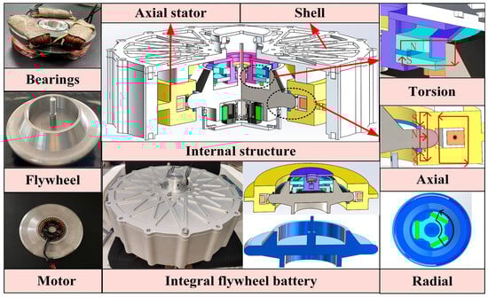
Figure 1. Flywheel structure and magnetic circuit diagram.

The magnetic circuit structure for axial flux is illustrated in the center-right portion of Figure 1. It adopts an axial hybrid magnetic bearing with a double permanent magnet up and down structure. The “additional air gap” beside the axial permanent magnet makes the magnetic circuit travel in accordance with the preset direction, which solves the problem of “self-loop” of the magnetic circuit of the permanent magnet and reduces the eddy current loss. The radial control flux is shown by the solid red line with an arrow in the lower right figure, which consists of three diameters at 120° intervals.

A three-phase AC current is applied to the radial control coil on the pole of the stator core to provide radial control flux. The three torsional stator poles form a “claw” distribution around the circle at 120-degree intervals. The solid black line with an arrow represents the axial control flux, which forms a loop between the axial stator of the radially tiled “C” structure, the axial spherical air gap, and the flywheel rotor, which also protects the failed flywheel.

In this paper, the operating conditions of the flywheel system under emergency avoidance are simulated, and the eccentricity of the operating conditions is investigated. When the vehicle is running for nine seconds, the vehicle begins to make emergency avoidance; that is, it starts to slow down in the ninth second, accompanied by sharp turns and side tilting of the vehicle. Therefore, at the ninth second, the fluctuations of the vehicle in the axial, radial, and torsional directions will be very severe.

2.2. Multiphysics Field Coupling Analysis

Table 1 provides the explanations of the concepts in this manuscript.

Table 1. The explanations of the concepts.

Term	Definition and Explanation
Cross-coupling situation	It refers to the complex state of interaction and influence among multiple physical fields, where a change in one field will simultaneously cause changes in multiple other fields. In a vehicle-mounted flywheel battery, mechanical vibration, temperature increase, and electromagnetic field changes occur simultaneously and intensify each other.
Extracted coupling characteristic function	The specific coupling analysis framework proposed in this paper takes into account the two-way interaction among the electromagnetic field, the temperature field, and the solid field. This is the most realistic high-fidelity model that closely resembles actual working conditions.
Unidirectional coupling	A simplified coupling analysis is conducted, where one physical field A affects another field B, but the changes in field B do not, in turn, affect field A.
Bidirectional coupling	A complete coupling analysis reveals that there is mutual feedback between physical fields A and B.
Solid field	It refers to the structural mechanical behavior of the research object, including the deformation, stress, strain, and vibration generated under the action of forces and thermal loads. In this article, “solid field” specifically refers to the structural responses of components such as flywheel rotors, bearings, and casing under the action of electromagnetic forces, thermal stresses, and inertial forces.
Bidirectional electromagnetic–thermal–solid coupling	From the “electromagnetic-thermal-solid bidirectional coupling” analysis results, one or a group of mathematical functions is extracted. This function can quantify the real-time intensity or state of the multi-field coupling and map it to an input that the controller can understand.

Different from previous studies that focused on the flywheel battery system in a single physical field, the focus of this research lies in investigating the impact of the bidirectional coupling relationship among multiple physical fields on the flywheel battery system. The condition of the track has the most direct impact on the stability of the vehicle-mounted flywheel battery. When the flywheel battery is affected, the active magnetic bearings are energized to stabilize the flywheel while generating a magnetic field and causing the temperature to rise. The increase in temperature causes the flywheel battery to deform. Therefore, the coupling relationship between the electromagnetic field and the temperature field is first analyzed. Subsequently, the coupling relationship between the electromagnetic field and the solid field is analyzed, and finally, the coupling relationship between the temperature field and the solid field is also examined; the working principle of the overall multi-field coupling analysis is shown in Figure 2.

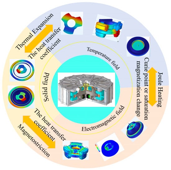
Figure 2. Multi-physical field coupling diagram.

(1)

Electromagnetic–Thermal Coupling Analysis

In the actual operation of the vehicle flywheel battery system, the flywheel is generally adjusted in real time by increasing the control current. In this way, the coil is energized and heated, and the current loss generated is the heat source of the thermal field. Heat is transferred to the material by radiation and convective heat transfer. At the same time, the airflow generated by the high-speed rotating flywheel rotor will carry away heat and change its temperature distribution. Correspondingly, the change in temperature will also affect the material’s electrical conductivity, gas density, dynamic viscosity, and thermal conductivity, thus affecting the current loss and gas flow rate. Therefore, there is an electric–heat flow–force interaction during operation: the magnetic field is the change and loss of the magnetic field caused by the electronation of the coil, the thermal field is the change in the temperature in the flywheel battery system caused by the Joule heat of the conducting coil, the flow field is the change in the heat radiation and heat convection heat transfer speed of the high-speed rotating flywheel rotor, and the force field is the unbalanced thermal stress and deformation caused by the high speed and temperature difference in the flywheel battery structure.

When the vehicle flywheel battery runs normally, the physical fields of the hybrid magnetic bearing interact with each other, and interact with each other. Flywheel eccentricity alters the magnetic field, which in turn induces losses, which causes the temperature to rise, and the loss caused by the magnetic field acting on the iron core during operation is also known as eddy current loss and magnetization loss. The average temperature curves of unidirectional coupling and bidirectional coupling are shown in Figure 3. It can be observed that the bidirectional coupling results in a higher temperature.

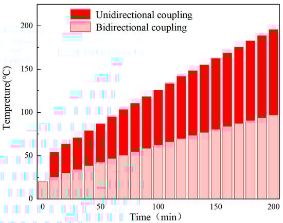
Figure 3. Multi-physical field coupling comparison diagram.

In the flywheel battery operation, the loss is mainly divided into copper consumption and iron consumption, where copper consumption P_c is

$$P_c=S{I}^{2}R{K}_S$$

(1)

In the equation, S is the number of phases, I is the stator winding current, R is the stator winding resistance, and K_s is the skin effect coefficient of the stator winding conductor.

Iron loss P_f is as follows:

$$P_f=P_h+P_c+P_e$$

(2)

In the equation, P_h denotes hysteresis loss, P_c is the eddy current loss, and P_e is an additional loss.

The main structure of a wheel battery is a magnetic bearing stator, flywheel rotor, winding, and permanent magnet. The material properties of the stator winding, iron core, and permanent magnet are easily affected by temperature changes, and the temperature of each part will change with time during operation.

The stator winding is made of copper, and its resistivity varies with the winding temperature. The winding temperature is affected by the change in winding resistivity, and the relationship between winding temperature and resistivity is complex. The relationship between temperature variation and winding resistivity is expressed as

$$\rho ={\rho }_0(1+\alpha (T-T_{ref}))$$

(3)

In the equation, $\rho$ is the actual winding resistivity, $\alpha$ is the temperature coefficient of copper, ${\rho }_0$ is the resistivity at the reference temperature, T is the winding temperature, T_ref is room temperature, T_ref = 20 °C.

Temperature will intensify the thermal motion within the silicon steel sheet material, resulting in an increase in the randomization of the magnetic moment direction, thus affecting the overall permeability. The relationship between permeability and temperature can be expressed as

$${\alpha }_{\mu }={\displaystyle \frac{{\mu }_{T2}-{\mu }_{T1}}{{\mu }_{T1}(T_2-T_1)}}$$

(4)

In the equation, μ_TI and μ_T2 are, respectively, the permeability at temperatures T₁ and T₂, and the unit is °C.

With the change in temperature, the magnetization of the permanent magnet increases as temperature changes occur, resulting in changes in magnetic properties. Here, the temperature coefficient of remanent magnetism α_Br and the temperature coefficient of intrinsic coercivity α_Hcj are

$$\left\{\begin{array}{l}{\alpha }_{Br}(t)={\displaystyle \frac{B_r(t)-B_{r20}}{B_{r20}(t-20)}}\times 100\%\\ {\alpha }_{Hcj}(t)={\displaystyle \frac{B_{cj}(t)-B_{cj20}}{B_{cj20}(t-20)}}\times 100\%\end{array}\right.$$

(5)

In the equation, t is the temperature of the permanent magnet, α_Br and α_Hcj are the temperature coefficients of remanent magnetism and the temperature coefficient of intrinsic coercivity at temperature t, respectively. B_r(t) and H_cj(t) are remanent magnetism and intrinsic coercivity at temperature t, respectively. B_r20 and H_cj20 are remanent magnetism and intrinsic coercivity at a temperature of 20 °C, respectively. The remanence temperature coefficients of flywheel batteries at different temperatures are shown in Figure 4.

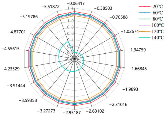
Figure 4. Permanent magnet coercive force diagram.

The effect of the temperature of a permanent magnet on the conductivity of a permanent magnet can be expressed as

$${\sigma }_m={\displaystyle \frac{{10}^6}{c{T}_{pm}+d}}$$

(6)

In the equation, c and d are constants, T_pm is the operating temperature of the permanent magnet, and the unit is °C.

Considering practical applications, the next step is to analyze the impact of air convection on copper loss.

Convection removes heat from the surface of the winding, reducing the steady-state temperature. Therefore, when convection intensifies, the coil temperature T_coil drops. The change in temperature of the coil ΔT_coil is

$$\Delta T_{coil}\approx {\displaystyle \frac{P_c+P_f}{h_{conv}\cdot A_{coil}}}-{\displaystyle \frac{P_{wind}}{h_{conv}\cdot A_{rotor}}}$$

(7)

In the equation, h_conv is the convective heat transfer coefficient, A is the heating dissipation surface area, and P_wind is the drag loss power.

The airflow directly cools the surface of the permanent magnet, with the temperature rising by 10 °C for each increment. The B_r value decreases by approximately 0.8% to 1.2%. Convection cooling can slow down the attenuation. Therefore, convective cooling reduces copper heat dissipation, creating a positive feedback cooling effect.

(2)

Electromagnetic-Solid Coupling Analysis

Ferromagnetic materials have a structure divided into magnetic domains, each of which is a uniformly magnetized region. When a magnetic field is applied, the boundaries between the domains move, and the domains rotate, both effects causing a change in the size of the material. When the object is magnetized, it will expand or contract in the direction of magnetization; the magnetostrictive coefficient is as follows:

$$\gamma ={\displaystyle \frac{L_H-L_0}{L_0}}$$

(8)

In the equation, L_H is the changed length of the magnetic material, and L₀ is the initial length of the magnetic material.

When magnetostriction is greater than zero, the material expands with the increase in magnetic field strength, and the magnetic coefficient is less than zero, and the material shortens with the increase in magnetic field strength. When magnetized, the length and volume should change slightly, and after removing the external magnetic field, the original length or volume is restored. It has three manifestations: the relative change in size along the direction of the external magnetic field, called longitudinal magnetostriction; the relative change in size perpendicular to the direction of the external magnetic field, called transverse magnetostriction; and the relative change in the volume size of a material, called volume magnetostriction.

Under the magnetization of a constant magnetic field, the relative elongation of the magnetic material is

$${\epsilon }_0={\displaystyle \frac{a{B}_0}{2}}$$

(9)

In the equation, ε₀ is the relative elongation of the magnetic material, B₀ is the magnetic induction intensity, and a is a constant that depends on the nature of the material.

If the external magnetic field is the superposition of a constant magnetic field and an alternating magnetic field, and the intensity of the constant magnetic field is much greater than that of the alternating magnetic field, the relative elongation of the magnetic material is

$$\epsilon =\beta B$$

(10)

In the equation, ε is the relative elongation of the magnetic material, B is the alternating magnetic field intensity, and β is the magnetic strain measurement, which depends on the nature of the material and constant magnetic field strength.

The magnetic properties of ferromagnetic materials change directionally under mechanical stress. This phenomenon is called the piezomagnetic effect.

The mechanical stress applied to ferromagnetic materials can be expressed by the following formula:

$$\sigma ={\displaystyle \frac{F}{S}}$$

(11)

In the equation, σ is stress, F is external mechanical force, S is effective cross-sectional area.

The relationship between the stress of magnetostrictive materials and the equivalent magnetic field can be expressed as

$$H_{\sigma }={\displaystyle \frac{9{\lambda }_{S}M}{2{\mu }_0{M}_S^2}}\sigma$$

(12)

In the equation, H_σ is the equivalent magnetic field generated by the change in magnetic permeability, λ_S is the magnetostriction constant, M_S is the saturation magnetization, M is the intensity of magnetization, and μ₀ is the permeability of vacuum.

The air-gap magnetic flux density varies dynamically due to changes in the air gap and temperature distribution. The winding inductance and resistance vary with temperature and cooling conditions, which affects the current response characteristics. Under the condition of air convection, the comprehensive influence formula of the electromagnetic force constant k_f can be expressed as

$$K_f(T,\delta )=K_{f0}\cdot {\displaystyle \frac{\mu (T)/{\mu }_0}{{(\delta /{\delta }_0)}^2}}$$

(13)

In the equation, K_f0 is the electromagnetic force constant at room temperature.

From this, it can be seen that if the convective cooling reduces the temperature rise by 20 °C and the air gap is reduced by 2 μm, then it may increase by approximately 3% to 5%.

(3)

Magnetic-solid Coupling Analysis

Due to the existence of temperature differences, heat will be transferred from high-temperature objects to low-temperature objects until the temperature equilibrium is reached. Therefore, according to the theory of heat transfer, the basic heat transfer modes are heat conduction, heat convection, and heat radiation. Heat conduction occurs due to the temperature gradient between objects, satisfying Fourier’s law.

$$Q=-\lambda S{\displaystyle \frac{\mathrm{d}T}{\mathrm{d}n}}$$

(14)

In the equation, Q is the heat transferred, λ is the thermal conductivity, S is the area, and T is the temperature.

The thermal conductivity of the material has a significant effect on the temperature variation. The stator and flywheel rotor in this study are made of silicon steel with a thermal conductivity of 40 W/(m·K).

In the heat transfer process, the shape of the solid also affects the temperature distribution. The rotor is a uniform, isotropic object. According to the three-dimensional coupled heat conduction theory, the expression of the volume strain under the axisymmetric structure is

$$e={\displaystyle \frac{\mathsf{\partial }{u}_r}{\mathsf{\partial }r}}+{\displaystyle \frac{u_r}{r}}+{\displaystyle \frac{\mathsf{\partial }{u}_z}{\mathsf{\partial }z}}$$

(15)

In the equation, e is the volume strain under the axisymmetric structure, u_r and u_z are the radial and axial components of the displacement vector, respectively.

The change in the volume of an object due to temperature variations. The formula for the deformation of an object can be expressed as

$$\Delta V=\beta \cdot V_0\cdot \Delta T$$

(16)

In the equation, ΔV is the variation in volume, β is the coefficient of volume expansion, V₀ is the volume of the object before the temperature change, and ΔT is the variation in temperature.

The coupling of airflow pressure pulsation and thermal deformation leads to a high-frequency and small-amplitude fluctuation of the air gap δ(t):

$$\delta (t)={\delta }_0+\Delta {\delta }_{thermal}(t)+\Delta {\delta }_{pressure}(t)$$

(17)

In the equation, Δδ_thermal(t) is the variation in the air gap caused by thermal deformation, and Δδ_pressure(t) is the variation in the air gap caused by the pressure pulsation of the airflow.

2.3. Multi-Field Coupling Results

The temperature distribution is shown in Figure 5. It can be observed from the temperature distribution diagram that the temperature distribution on the radial stator and flywheel rotor is very uneven, which is related to the distribution of current. The temperature on the radial stator is mainly distributed in the control coil, where the heat is too late to diffuse to a deeper depth, and the position is easier to form a high temperature area than other positions.

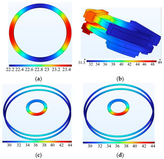
Figure 5. Temperature distribution diagram: (a) Temperature of axial stator. (b) Temperature of radial and torsional stator. (c) Temperature of radial and axial permanent magnet. (d) Temperature of flywheel.

When the dynamic eccentricity of the flywheel rotor is 40%, the change in temperature of each component of the flywheel battery with time under rated operating conditions can be found that the stator and coil temperatures are the highest, and the temperature change is the greatest.

The changes in temperature of each part of the flywheel battery system over time are shown in Figure 6. It can be observed that as time increases, the temperature gradually rises.

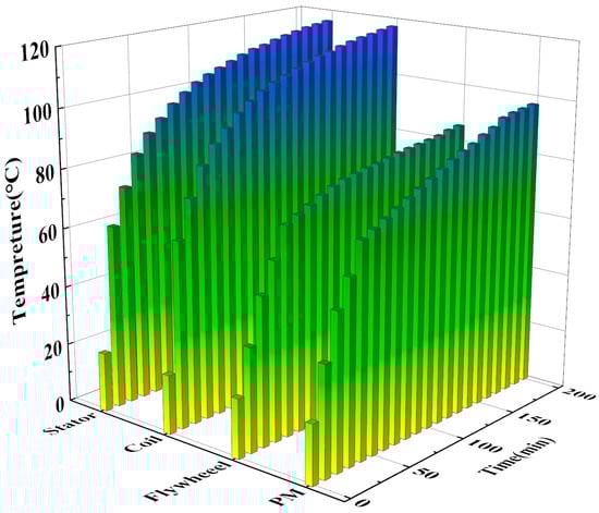
Figure 6. Temperature curve of each part of the magnetic bearing.

The air gap change is shown in Figure 7. It can be observed that the coupling effects of flywheel rotor speed factors on the radial stator outer diameter deformation and the coupling effects on the rotor inner deformation are modeled as a polynomial at the highest temperature. The results of the magnetostrictive deformation of the radial stator and flywheel are shown in Figure 8. It can be observed that the maximum deformation of the stator is 0.75 μm and the maximum deformation of the flywheel is 0.435 μm.

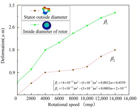
Figure 7. Air gap change diagram.

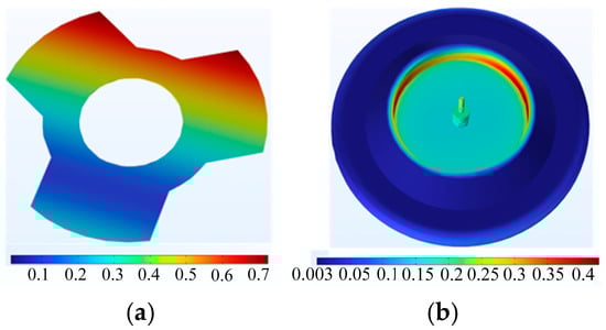
Figure 8. Magnetostrictive deformation of (a) radial stator and (b) flywheel.

The distribution of magnetic field density is shown in Figure 9. It can be observed that the magnetic field distribution starts from the stator, goes to the flywheel, and then returns to the stator, forming a closed loop.

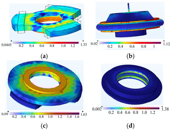
Figure 9. Magnetic field distribution diagram of flywheel. (a) Magnetic flux density distribution of radial stator. (b) Magnetic flux density distribution of axial permanent magnet and flywheel. (c) Magnetic flux density distribution of twist. (d) Magnetic flux density distribution of radial stator.

2.4. The Influence of Multiple Coupling Effects on the Performance of the Control System

According to Equations (4) and (11), an increase in temperature by ΔT will lead to a change in magnetic permeability of Δμ, which in turn will affect the electromagnetic force constant K_f :

$$K_f(T)=K_{f0}\cdot [1+{\alpha }_{\mu }(T-T_0)]$$

(18)

In the equation, k_f0 is the electromagnetic force constant at room temperature, and α_μ is the temperature coefficient of magnetic permeability. When the temperature rises from 20 °C to 40 °C, the calculated change in the electromagnetic force constant is approximately 6 percent. This results in a need for an approximately 15% increase in control gain to maintain the same stiffness.

The coupling strength index is

$$\eta =\left|{\displaystyle \frac{\Delta K_f}{K_{f0}}}\right|+\left|{\displaystyle \frac{\Delta \delta }{{\delta }_0}}\right|+\left|{\displaystyle \frac{\Delta B_{sat}}{B_{sat0}}}\right|$$

(19)

In the equation, ΔK_f is the variation in the electromagnetic force constant, K_f0 is the electromotive force constant at normal temperature, ΔB_sat is the change in magnetic field density, and B_sat0 is the saturation magnetic density at room temperature. The quantitative impact of multiple coupling parameter changes on control performance is summarized in Table 2.

Table 2. The influence of multiple coupling parameter changes on control performance.

Coupling Effect	Change in Physical Quantity	The Influence on Control Parameters
ΔT	20 °C	kf increased by 7%
Δδ	0.75 μm	Almost no impact
ΔB	8%	Current limit needs to be increased by 10%

In conclusion, if no parameter adaptive adjustment is made, the steady-state error will increase by 10–12%, the overshoot amount will increase by 5–8%, the time must be adjusted by extending it by 10–15%, and the time for the sliding mold to arrive must be extended by 11%.

Based on the results of multi-field coupling, we have extracted a coupling characteristic function that can link the changes in physical fields with control parameters. This function will be used in Section 3 to design an extremely robust sliding mode controller. Based on the results of Section 2.3, the coupled characteristic functions derived map the real-time changes in temperature, deformation, and flux into the control parameters of the sliding mode. This enables the controller to dynamically adapt to the multi-physics field coupling effects.

3. Highly Robust Control Strategy Based on Coupling Characteristic Function

3.1. Overall Control System Design

The overall block diagram of the control is shown in Figure 10. This paper mainly studies the sliding mode controller part of the control and the parameter selection of sliding mode control. In the sliding mode control design, the results of the multiphysics field coupling analysis are integrated with the sliding mode control parameters to formulate a unified coupling characteristic function. By monitoring the real-time variations in the multiphysics coupling results, the optimal control parameters can be determined at each time instant, thereby enabling real-time optimal parameter tuning for the sliding mode controller.

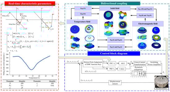
Figure 10. Block diagram of sliding mode control strategy.

The mathematical model of the axial magnetic bearing was established. The forms of magnetic flux and control current were designed as

$$m\ddot{x}={\displaystyle \frac{{\mu }_{0}S{(F_m-2Nu)}^2}{8{(x_0-x)}^2}}+{\displaystyle \frac{{\mu }_{0}S{(F_m+2Nu)}^2}{8{(x_0+x)}^2}}-G+f$$

(20)

In the equation, G is the gravity of the flywheel, and f is the external disturbance force acting on the flywheel. For this system, the model of a time-varying affine nonlinear system using Taylor series is expanded by the nonlinear function (21) with respect to u(t) around the time-varying linearized point µ. The final results are shown in the following:

$$\left\{\begin{array}{c}{\dot{x}}_1=x_2\\ {\dot{x}}_2=f_n(x_1,\mu )+u\cdot h_n(x_1,\mu )+d(t)\\ y=x_1\end{array}\right.$$

(21)

$$\left\{\begin{array}{c}\begin{array}{c}{f}_n(x_1,\mu )=f_m(x_1,\mu )-\mu \cdot h_n(x_1,\mu )\end{array}\\ \begin{array}{c}{f}_m(x_1,\mu )={\displaystyle \frac{K}{m}}\left({\displaystyle \frac{{(F_m-2n\mu )}^2}{{(x_0-x_1)}^2}}+{\displaystyle \frac{{(F_m+2n\mu )}^2}{{(x_0+x_1)}^2}}\right)\end{array}\\ h_n(x_1,\mu )=-{\displaystyle \frac{{\mu }_{0}nS}{2m}}\left({\displaystyle \frac{F_m-2n\mu }{{(x_0-x_1)}^2}}-{\displaystyle \frac{F_m+2n\mu }{{(x_0+x_1)}^2}}\right)\end{array}\right.$$

(22)

In the equation, m is the mass of flywheel, x is the actual displacement of flywheel rotor, x₁ = x, x₂ = x, x₀ is the length of air gap at axial equilibrium position, µ₀ is the vacuum permeability, S is the cross-sectional area of magnetic pole, F_m is the total magnetomotive force of axial PMs, n is the number of axial coils, u is the axial control current, µ is the time-varying linearized point, should be as close to u as possible, u · (t − 1) = µ, and d(t) is the external disturbances and |d(t)| ≤ D.

The controller of the magnetic bearing is designed based on a sliding mode control strategy. Let the expected displacement of the flywheel be x_r, the actual displacement be x₁, and the error be e = x_r − x₁; the sliding mode function is designed as

$$s=\dot{e}+ce$$

(23)

In the equation, c > 0, taking the derivative of (20) and plugging it into the value of (21), which can be obtained as follows:

$$\dot{s}={\ddot{x}}_r-f_n(x_1,\mu )-u\cdot h_n(x_1,\mu )-d(t)+c({\dot{x}}_1-{\dot{x}}_r)$$

(24)

The approach law of SMC is designed as

$$\dot{s}=-\epsilon \mathrm{sgn}(s), \mathrm{sgn}(s)=\{-1,s<0; 0,s=0; 1,s>0\}$$

(25)

In the equation, ε shows the approach rate and ε > 0, and combining (24) and (25), the controller can be designed to

$$u_s={\displaystyle \frac{1}{h_n(x_1,\mu )}}\left({\ddot{x}}_r-f_n(x_1,\mu )+c({\dot{x}}_1-{\dot{x}}_r)+\epsilon \cdot \mathrm{sgn}(s)\right)$$

(26)

The Lyapunov function is chosen as L = s²/2; therefore,

$$\begin{array}{l}\dot{L}=s\dot{s}=s\left({\ddot{x}}_r-f_n(x_1,\mu )-u\cdot h_n(x_1,\mu )-d(t)+c({\dot{x}}_1-{\dot{x}}_r)\right)\\ =s\left(\begin{array}{l}{\ddot{x}}_r-\left({\ddot{x}}_r-f_n(x_1,\mu )+\epsilon \cdot \mathrm{sgn}(s)+c({\dot{x}}_1-{\dot{x}}_r)\right)\\ -f_n(x_1,\mu )-d(t)+c({\dot{x}}_1-{\dot{x}}_r)\end{array}\right)\\ =s\cdot d(t)-\epsilon \left|s\right|\end{array}$$

(27)

When choosing ε ≥ D, $s\dot{s}$ ≤ 0 is obtained. At this point, the system will converge gradually and stably, and has good robustness. Because of the sgn(s) function, this section of SMC is not continuous, and the moving point of sliding mode cannot accurately reach the pre-designed sliding mode surface, but shuttles back and forth on both sides of the sliding mode surface. Therefore, a status monitor is designed based on SMC. The principle is to select a boundary layer with a thickness of ζ near the sliding mode surface. When s ≥ ζ, the controller is set to u = m(s) · u_s, and when s < ζ, the controller is set to PID output up. The purpose is to switch to a smooth transition of the PID output when the moving point of the sliding is reached. It reaches near the sliding mode surface and avoids buffeting. The status monitor m(s) is designed as

$$m(s)=\left\{\begin{array}{l}1, \left|s\right|\ge \zeta \\ {\displaystyle \frac{\left|s\right|}{\zeta }}, \left|s\right|<\zeta \end{array}\right.$$

(28)

Therefore, the final controller is designed as

$$\left\{\begin{array}{l}u=\left\{\begin{array}{l}m(s)\cdot u_s, \hspace{1em}\hspace{1em}\hspace{1em}\left|s\right|\ge \zeta \\ \left(1-m(s)\right)\cdot u_p,\hspace{1em}\left|s\right|<\zeta \end{array}\right.\\ u_s={\displaystyle \frac{1}{h_n(x_1,\mu )}}\left({\ddot{x}}_r-f_n(x_1,\mu )+c({\dot{x}}_1-{\dot{x}}_r)+\epsilon \cdot \mathrm{sgn}(s)\right)\\ u_p=k_p\left(e+T_i{\displaystyle {\int }_0^{t}e\mathrm{d}t}+T_d\dot{e}\right)\\ e=x_r-x_1\end{array}\right.$$

(29)

In the vicinity of the flywheel’s equilibrium point, the controller utilizes linear PID control. Only when the displacement exceeds the linearization range does it switch to nonlinear sliding mode control to restore the flywheel to its equilibrium position.

The switching mechanism in the manuscript can effectively suppress jitter, but it also introduces stability issues in the switching region. The following analysis is conducted from the perspectives of Lyapunov stability theory and switching system theory.

Constructing the Lyapunov function,

$$V={\displaystyle \frac{1}{2}}{s}^2+{\displaystyle \frac{1}{2}}\lambda {\left(\int edt\right)}^2$$

(30)

Taking the derivative and substituting it into the PID control law, we obtain

$$\dot{V}=s\dot{s}+\lambda e\int edt$$

(31)

By appropriately selecting the PID parameters, asymptotic stability can be achieved within the boundary layer.

The continuous switching function employed in this manuscript is applied at s = ±ξ; at this point, the output of the controller is

$$u=m(s)u_s+(1-m(s))u_p$$

(32)

Within the boundary layer, although PID control does not possess the complete disturbance invariance of sliding mode control, its linear characteristics and integral action can still effectively suppress low-frequency disturbances to a certain extent. Moreover, when the disturbance causes ∣s∣ ≥ ζ, the system will rapidly switch to sliding mode control and re-enter the strong robust region, thereby ensuring the overall stability of the system under complex operating conditions. Therefore, it avoids system jitter or instability caused by sudden changes in input.

When the system state is far from the equilibrium point (indicated by a large sliding variable), the nonlinear SMC is activated. The SMC is chosen for this regime due to its inherent robustness to model uncertainties and external disturbances, enabling it to forcefully drive the system back towards the desired trajectory despite the nonlinearities and coupling effects exacerbated by large displacements.

Once the system state enters the vicinity of the equilibrium point (within the boundary layer), control authority is handed over to a linear PID controller. Within this small region, the system dynamics can be approximately linearized. The PID controller provides smooth and precise control without the high-frequency chattering typical of SMC, which is beneficial for reducing unnecessary actuator wear and improving steady-state accuracy.

Table 3 summarizes the influence of control parameters on the control system. It is found that the Reaching Law Coefficient ε has the greatest impact on the control system. Therefore, it is selected to be associated with the temperature. This design introduces minimal computational overhead to the CPU.

Table 3. The influence of control parameters.

Parameter	Degree of Importance	Impact on the System
ε	5	Dynamic response speed and robustness
c	4	The threshold for the smooth switching between sliding mode control and PID control
ξ	3	The dynamic convergence form of tracking error

3.2. Parameter Extraction and Coupling Characteristic Function

The parameter extraction architecture adopts a hierarchical progressive, physically driven, and real-time optimization design principle, gradually refining the original multi-sensor data into low-dimensional feature vectors suitable for control decisions. The entire process is divided into four processing stages. Firstly, hardware-triggered synchronous sampling and a unified clock source trigger all ADCs to convert simultaneously ensure the synchronous acquisition mechanism. Then, data preprocessing and quality control will be carried out, following the calculation of physical coupling characteristics. Finally, fusions are carried out.

Regarding the processing of data, remove the DC bias in sequence, apply anti-aliasing filtering, and perform detection and correction for outliers.

The elimination of DC bias is as follows:

$$\tilde{x}(t)=x_{\mathrm{raw}}(t)-{\displaystyle \frac{1}{N}}\sum _{i=k-N+1}^k{x}_{\mathrm{raw}}(t_i)$$

(33)

In the equation, x_raw(t) is the original sensor reading, $\tilde{x}(t)$ is the signal after removing the DC component, and N is the sliding average window length.

The anti-aliasing filter is as follows:

$$x_{\mathrm{filt}}(t)=H_{\mathrm{LP}}(s)\ast \tilde{x}(t),\hspace{1em}{f}_c=2\mathrm{kHz}$$

(34)

In the equation, H_LP(s) is the transfer function of the low-pass filter; f_c is the cut-off frequency.

The outlier detection and correction are as follows:

$$x_{\mathrm{clean}}(t_k)=\left\{\begin{array}{c}\mathrm{median}\{x(t_{k-2}),x(t_{k-1}),x(t_{k+1}),x(t_{k+2})\},\mathrm{if}|x(t_k)-{\mu }_{100}|>3{\sigma }_{100}\\ x(t_k), \hspace{1em}\hspace{1em}\hspace{1em}\hspace{1em}\hspace{1em}\hspace{1em}\hspace{1em}\hspace{1em}\mathrm{otherwise}\end{array}\right.$$

(35)

In the equation, μ₁₀₀ is the sample mean of the most recent 100 points. σ₁₀₀ is the sample standard deviation of the last 100 points.

The calculation of the physical coupling characteristics requires the calculation of the three coupling strength indicators mentioned in the second part.

The electromagnetic–thermal coupling strength index is as follows:

$${\Gamma }_{\mathrm{ET}}(t_k)={\displaystyle \frac{P_{\mathrm{loss}}}{P_{\mathrm{in}}}}\times {\displaystyle \frac{T_{\max }(t_k)-T_{\max }(t_{k-L})}{\Delta t\cdot L}}\times e^{-T_{\max }/T_{ref}}$$

(36)

In the equation, P_loss/P_in is the power loss ratio, Δt is the sampling interval, L is the window length, and T_ref is the range of temperature.

Thermal–mechanical deformation coupling:

$${\Gamma }_{\mathrm{TM}}(t_k)={\displaystyle \frac{T_{\max }-T_{\min }}{T_{\mathrm{avg}}}}\times {\displaystyle \frac{{\sigma }_{\delta }^2}{{\delta }_{\mathrm{nom}}^2}}\times {\beta }_{\mathrm{cff}}(T_{\mathrm{avg}})$$

(37)

In the equation, δ_nom is nominal air gap and β_eff is effective thermal expansion coefficient.

The electromechanical coupling index is as follows:

$${\Gamma }_{\mathrm{EM}}(t_k)=\left|{\displaystyle \frac{\mathrm{Cov}[B(t),\delta (t)]}{{\sigma }_B{\sigma }_{\delta }}}\right|\times {\displaystyle \frac{I_{\mathrm{rms}}}{I_{\mathrm{rated}}}}$$

(38)

In the equation, Cov[B,δ] is the covariance, σ_B is the magnetic field standard deviation, and σ_δ is the displacement standard deviation; I_rms/I_rated is the current load factor.

The formula for characters fusion index is as follows:

$$\begin{gathered} {\varphi }_1(t_k)=w_{11}{z}_1+w_{12}\left({\displaystyle \frac{T_{\max }-T_0}{T_{\lim }-T_0}}\right)+w_{13}\left|{\displaystyle \frac{\overline{\delta }}{{\delta }_{nom}}}-1\right| \\ {\varphi }_2(t_k)=w_{21}{z}_2+w_{22}\left({\displaystyle \frac{{\sigma }_{\delta }}{{\delta }_{\mathrm{nom}}}}\right)+w_{23}\left({\displaystyle \frac{I_{\mathrm{rms}}}{I_{\mathrm{rated}}}}\right) \\ {\varphi }_3(t_k)=w_{31}{z}_3+w_{32}{\displaystyle \frac{\omega }{{\omega }_{\mathrm{rated}}}}+w_{33}{\Gamma }_{\mathrm{ET}} \end{gathered}$$

(39)

In the equation, w_ij is the integration weight coefficient, T_lim is the upper temperature limit, and δ_nom is the nominal air gap.

The adaptive normalization formula is as follows:

$${\varphi }_{\mathrm{norm}}(t_k)={\displaystyle \frac{\varphi (t_k)-{\mu }_{\mathrm{hist}}(k)}{{\sigma }_{\mathrm{hist}}(k)+ϵ}}$$

(40)

In the equation, ϕ_norm is the normalized feature vector, μ_hist is the historical mean vector, and σ_hist is the historical standard deviation vector.

By adopting the method of establishing a real-time, nonlinear function relationship from the physical state space to the controller parameter space, the mapping process of the multi-physics coupling characteristics to the control gain is achieved. This process first goes through the offline training stage, based on a large amount of multi-physics coupling simulation and experimental data, to construct a corresponding relationship database between the coupling characteristics vector and the optimal control gain. Then, the radial basis function neural network (RBFNN) is used to learn and generalize this mapping relationship, forming the core mapping function. During the online execution phase, the system calculates the current coupling characteristics in real time and predicts the initial gain through the mapping function. Subsequently, it enforces the hard constraints composed of stability theory and physical constraints for correction. Then, it undergoes dynamic smoothing processing (such as limiting the rate of change) to prevent gain jumps. Finally, it outputs the real-time optimized control gain.

The mapping function of the proximity coefficient ϵ(t):

$$ϵ(t)={ϵ}_0\cdot \left[1+k_1\cdot \tanh \left({\displaystyle \frac{{\Gamma }_{\mathrm{total}}(t)}{{\Gamma }_0}}\right)\right]\cdot \left[1+k_2\cdot {\displaystyle \frac{|s(t)|}{s_{\max }}}\right]$$

(41)

In the equation, Γ₀ is the coupling strength reference value, Γ_total is the coupling strength, and k₁ and k₂ are gain factors.

The mapping function of the sliding surface coefficient c(t) is as follows:

$$c(t)=c_0\cdot \left[1+{\lambda }_1\cdot {\displaystyle \frac{\parallel \nabla T(t)\parallel }{\parallel \nabla T{\parallel }_{\max }}}+{\lambda }_2\cdot {\displaystyle \frac{|de/dt|}{|de/dt{|}_{\max }}}\right]$$

(42)

In the equation, c₀ is the fiducial value, and k1, λ₁, and λ₂ are weight coefficients.

The mapping function of the boundary layer thickness ξ(t) is as follows:

$$\zeta (t)={\zeta }_0\cdot \left[1-{\mu }_1\cdot {\displaystyle \frac{{\Gamma }_{TM}(t)}{{\Gamma }_{TM,\max }}}+{\mu }_2\cdot {\displaystyle \frac{|e(t)|}{e_{\max }}}\right]$$

(43)

In the equation, μ₁ and μ₂ are weight coefficients. ξ₀ is the mapping function of the boundary layer thickness reference value, Γ is the coupling strength, and e is the error.

As illustrated in Figure 11. This relationship was obtained from extensive offline coupling simulations, ensuring that the controller’s aggressiveness is scaled appropriately with the intensity of the internal coupling effects.

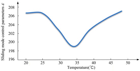
Figure 11. Real-time characteristic parameters.

Therefore, we can determine the quantity of sliding mode control parameters. Table 2 shows the reference values of control parameters of the flywheel battery control system under various road conditions.

For Table 4, the values of N, F_m, and μ are determined based on the actual parameters of the prototype of vehicle-mounted flywheel battery in following experiments; c is the coefficient of the sliding mode function; ε is the approach rate of SMC, where the sliding mode controller is debugged according to its response during simulation and parameters are determined under relatively optimal control performance; and ζ is the thickness of the output switching boundary layer of SMC and PID, where the parameter is selected to ensure the smooth switching of the controller output.

Table 4. Control parameters of the flywheel battery control system.

Parameter	Quantity
N	290
$F_m$	0.1
μ	25
c	200
ξ	0.02

4. Experiment and Result

In the experiment, the real-time characteristic parameters are updated based on the coupling function derived in Section 3, which itself is built upon the multi-physics results from Section 2.3. This enables the controller to respond to road-induced disturbances more effectively than fixed-parameter controllers.

4.1. Experiment Platform

The experimental platform is used to simulate various road conditions that real cars may encounter on the road. The whole experimental platform is shown in Figure 12. This experimental platform is composed of an upper computer, power supply vehicle, flywheel battery system, magnetic suspension control system, auxiliary power distribution system, and test system.

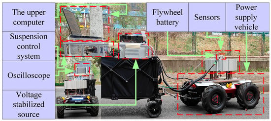
Figure 12. Experimental platform.

The flywheel battery, mounted on the power supply vehicle, provides power to the electric car. The flywheel rotor in the flywheel battery is suspended by magnetic bearings. A sensor positioned directly above the flywheel detects its real-time position. At the rear of the power supply vehicle is the control system of the flywheel battery. At the top is the upper computer, and below the upper computer is the magnetic levitation control system, which is used to control the normal operation of the flywheel battery system. On the right side of the suspension control system are, respectively, a voltage stabilized source for powering the control system and an oscilloscope for displaying the waveforms of sensors, which are used to present the real-time position of the flywheel.

In order to make the experimental conditions more complete, this manuscript provides detailed parameters of the experimental vehicles. The parameters are shown in Table 5.

Table 5. Parameters of the experimental vehicles.

Parameter	Quantity
Dimension	820 × 640 × 310 MM
Weight	42 kg
Velocity	5 m/s
Braking Length	2 M
Power Supply	24 V/15 A

4.2. Performance Test

To validate the superiority of the sliding mode control system with real-time characteristic parameters over that with fixed optimal parameters, the selection of road conditions should ensure that the vehicle speed and position are constantly changing. Therefore, the emergency avoidance condition is selected in this study. And the speed of the flywheel rotor is set to 1500 rpm. The specific road profile is depicted in Figure 13.

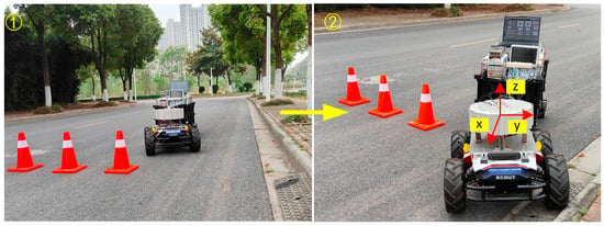
Figure 13. Experimental road conditions.

First, the vehicle travels at a constant speed on the road, and then, the vehicle encounters an obstacle and applies emergency braking and turns. Finally, part of the vehicle remains on the short slope where the steps intersect the road surface.

The displacement waveforms from the emergency-avoidance road condition experiment using optimal parameters are shown in Figure 14. In Figure 14, (a) represents displacement in x₁ direction, (b) represents displacement in y₁ direction, (c) represents displacement in x₂ direction, (d) represents displacement in y₂ direction, and (e) represents displacement in z direction. The displacement waveforms of the emergency-avoidance road-condition experiment with the optimal-parameter sliding mode control system are shown in Figure 15. In Figure 15, (a) represents displacement in x₁ direction, (b) represents displacement in y₁ direction, (c) represents displacement in x₂ direction, (d) represents displacement in y₂ direction, and (e) represents displacement in z direction.

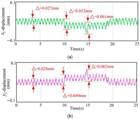
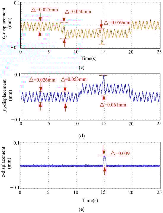
Figure 14. Displacement waveforms from the emergency avoidance experiment using the sliding mode controller with fixed optimal parameters. (a) Displacement in x₁ direction, (b) displacement in y₁ direction, (c) displacement in x₂ direction, (d) displacement in y₂ direction, and (e) displacement in z direction.

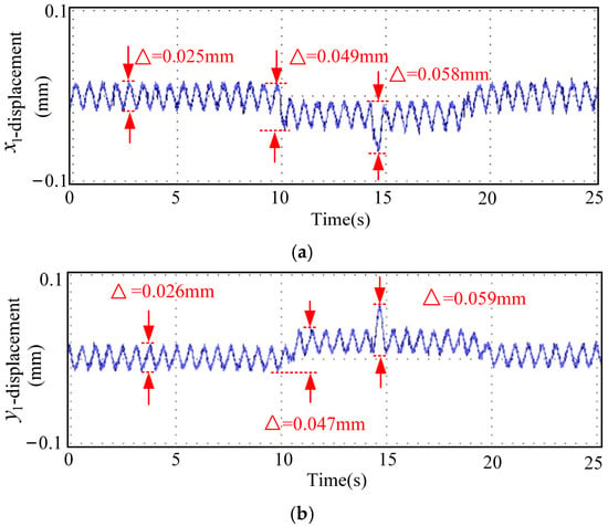
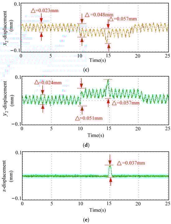
Figure 15. Waveforms of emergency-avoidance road-condition experiment sliding mode control system with real-time characteristic parameters. (a) Displacement in x₁ direction, (b) displacement in y₁ direction, (c) displacement in x₂ direction, (d) displacement in y₂ direction, and (e) displacement in z direction.

By comparing Figure 14 and Figure 15, the RMSE of the real-time parameters SMC in all directions has decreased by approximately 50%, indicating that the real-time adjustment of parameters based on the multi-physics field coupling characteristic function significantly improves the tracking accuracy of the system. The average stabilization time of the real-time parameter SMC has been shortened by approximately 35%, indicating that the system can recover to a stable state more quickly after being subjected to external disturbances and has a better dynamic response. The overshoot of the real-time parameter SMC has been reduced by approximately 50% to 60%, indicating that the oscillations during the transient process of the system have significantly decreased, and the robustness has improved.

In conclusion, the real-time parameter SMC control strategy based on multi-physics field coupling characteristic functions outperforms the fixed-parameter SMC strategy in terms of tracking accuracy, dynamic response speed, and stability.

5. Conclusions and Future Work

5.1. Conclusions

In this study, a real-time mapping mechanism is established from the multi-physical field coupling state to the parameters of the sliding mode controller, achieving adaptive gain adjustment without relying on an accurate system model. This provides a new approach driven by physical characteristics for the control of strongly coupled time-varying systems. This method has the advantages of fast response, low computational complexity, and ease of engineering implementation. Experimental results show that this strategy significantly improves the tracking accuracy, response speed, and robustness of the system. Future work will further deepen the analysis of multi-physical field coupling and the integration of control parameters, and verify and expand the applicability of this method in a wider range of operating conditions and system levels.

5.2. Future Work

Although the proposed electromagnetic–thermal–solid two-way coupling analysis method and the control strategy based on coupled characteristic functions in this study have demonstrated excellent performance in enhancing system robustness, it is necessary to point out that the coupling equation solution method adopted in this paper is still based on certain simplified assumptions. When dealing with extremely complex geometric structures or strong nonlinear physical behaviors, there may be accuracy limitations. For example, when the flywheel battery has a highly asymmetric design or the material enters the deep saturation zone, the analytical model may not be able to fully capture its dynamic characteristics.

Future research could consider incorporating high-fidelity discretization simulation tools (such as the finite element method and computational fluid dynamics) to more accurately depict complex geometries and nonlinear effects. At the same time, to overcome the high computational cost issue caused by this, the proxy model technology proposed in reference [7] (such as neural networks, Gaussian process regression, etc.) can be adopted to construct a “simulation-proxy” hybrid model framework.

References

- Zhang, W.Y.; Wu, T.; Zhou, W.J. Accurate Modeling of Saucer-Shaped Flywheel Battery Based on Magnetic Field Estimation and Virtual Air Gap Transformation. IEEE Trans. Ind. Electron. 2025, 72, 10411–10422. [Google Scholar] [CrossRef]
- Moraes, C.G.D.S.; Brockveld, S.L.; Heldwein, M.L.; Franca, A.S.; Vaccari, A.S.; Waltrich, G. Power Conversion Technologies for A Hybrid Energy Storage System in Diesel-electric Locomotives. IEEE Trans. Ind. Electron. 2021, 68, 9081–9091. [Google Scholar] [CrossRef]
- Wu, T.; Zhang, W. Review on Key Development of Magnetic Bearings. Machines 2025, 13, 113. [Google Scholar] [CrossRef]
- Zhang, W.Y.; Gu, X.W.; Ji, H.T. Robust Sensorless Control of Vehicle-Mounted Flywheel Battery Against Continuous Road Disturbances. IEEE Trans. Transp. Electrific. 2025, 11, 12052–12062. [Google Scholar] [CrossRef]
- Zhang, W.Y.; Wang, J.W.; Li, A.; Xiang, Q.W. Multiphysics Fields Analysis and Optimization Design of a Novel Saucer-Shaped Magnetic Suspension Flywheel Battery. IEEE Trans. Transp. Electrific. 2024, 10, 5473–5483. [Google Scholar] [CrossRef]
- Sun, M.X.; Xu, Y.L.; Zhang, W.J. Multiphysics Analysis of Flywheel Energy Storage System Based on Cup Winding Permanent Magnet Synchronous Machine. IEEE Trans. Energy Convers. 2023, 38, 2684–2694. [Google Scholar] [CrossRef]
- Gong, L.; Zhu, C.S. The Influence of PID Controller Parameters on Polarity Switching Control for Unbalance Compensation of Active Magnetic Bearings Rotor Systems. IEEE Trans. Ind. Electron. 2024, 71, 8324–8338. [Google Scholar]
- Praslicka, B.; Ma, C.; Taran, N. A Computationally Efficient High-Fidelity Multi-Physics Design Optimization of Traction Motors for Drive Cycle Loss Minimization. IEEE T. Ind. Appl. 2023, 59, 1351–1360. [Google Scholar] [CrossRef]
- Jiang, S.; Zhou, B.; Huang, X.; Wang, K.; Xu, L. 3-D Global Thermal Analysis of DSEM Considering The Temperature Difference Between Excitation and Armature Coils. IEEE Trans. Ind. Electron. 2021, 68, 11931–11940. [Google Scholar] [CrossRef]
- Kumar, T.R.D.; Mija, S.J. Boundary Logic-based Hybrid PID-SMC Scheme for A Class of Underactuated Nonlinear Systems-Design and Real-Time Testing. IEEE Trans. Ind. Electron. 2025, 72, 5257–5267. [Google Scholar] [CrossRef]
- Qiang, H.; Cheng, X.; Huang, H.; Hai, Y.; Sun, Y. Yaw Feedback Control of Active Steering Vehicle Based on Differential Flatness Theory. J. Theor. Appl. Mech. 2025, 63, 131–-149. [Google Scholar] [CrossRef]
- Zhao, X.; Sun, Y.; Sun, W.; Xu, J.; Lin, G. Safe Reinforcement Learning Control for Maglev Train Levitation System with Stability Guarantee and Safety Constraint. IEEE Trans. Transp. Electrific. 2026, 12, 285–296. [Google Scholar] [CrossRef]
- Wei, Y.; Young, H.; Ke, D.; Wang, F.; Qi, H.; Rodríguez, J. Model-Free Predictive Control Using Sinusoidal Generalized Universal Model for PMSM Drives. IEEE Trans. Ind. Electron. 2024, 71, 13720–13731. [Google Scholar] [CrossRef]
- Shen, J.; Liu, Y.; Wang, W.; Wang, Z. Composite Learning Adaptive Safety Critical Control with Application to Adaptive Cruise of Intelligent Vehicles. IEEE Trans. Ind. Electron. 2025, 72, 10793–10803. [Google Scholar] [CrossRef]
- Hou, Q.; Wang, H.; Lee, C.H.T.; Ding, S. Composite Adaptive Super-Twisting Sliding Mode Control Using Barrier Function for PM Motor Drives toward Electric Aircraft Applications. IEEE Trans. Power Electron. 2025, 40, 16255–16264. [Google Scholar] [CrossRef]
- Hou, Q.; Ding, S.; Yu, X.; Mei, K. A Super-Twisting-Like Fractional Controller for SPMSM Drive System. IEEE Trans. Power Electron. 2022, 69, 9376–9384. [Google Scholar] [CrossRef]
- Sun, J.L.; Wang, Z.; Ding, S.H.; Xia, J.; Xing, G.Y. Adaptive Disturbance Observer-based Fixed Time Nonsingular Terminal Sliding Mode Control for Path-tracking of Unmanned Agricultural Tractors. Biosyst. Eng. 2024, 246, 96–109. [Google Scholar] [CrossRef]
- Lian, S. Adaptive Attitude Control of a Quadrotor Using Fast Nonsingular Terminal Sliding Mode. IEEE Trans. Ind. Electron. 2022, 69, 1597–1607. [Google Scholar] [CrossRef]
- Zhang, W.Y.; Li, Z.B. Trajectory Tracking Control Based on NP-RMPC with the Uncertain Model Parameters for Magnetic Bearing-Rotor System. IEEE Trans. Ind. Electron. 2025, 11, 11563–11574. [Google Scholar] [CrossRef]
- Alipour, M.; Zarei, J.; Razavi-Far, R.; Saif, M.; Mijatovic, N.; Dragičević, T. Observer-Based Backstepping Sliding Mode Control Design for Microgrids Feeding A Constant Power Load. IEEE Trans. Ind. Electron. 2023, 70, 465–473. [Google Scholar] [CrossRef]
- Wang, Y.; Feng, Y.; Zhang, X.; Liang, J. A New Reaching Law for Antidisturbance Sliding-Mode Control of PMSM Speed Regulation System. IEEE Trans. Power Electron. 2020, 35, 4117–4126. [Google Scholar] [CrossRef]
- He, L.; Wang, F.; Ke, D. FPGA-Based Sliding-Mode Predictive Control for PMSM Speed Regulation System Using an Adaptive Ultra-Local Model. IEEE Trans. Power Electron. 2021, 36, 5784–5793. [Google Scholar] [CrossRef]
- Çavuş, B.; Aktaş, M. A New Adaptive Terminal Sliding Mode Speed Control in Flux Weakening Region for DTC Controlled Induction Motor Drive. IEEE Trans. Power Electron. 2024, 39, 449–458. [Google Scholar] [CrossRef]
Disclaimer/Publisher’s Note: The statements, opinions and data contained in all publications are solely those of the individual author(s) and contributor(s) and not of MDPI and/or the editor(s). MDPI and/or the editor(s) disclaim responsibility for any injury to people or property resulting from any ideas, methods, instructions or products referred to in the content. |
© 2026 by the authors. Licensee MDPI, Basel, Switzerland. This article is an open access article distributed under the terms and conditions of the Creative Commons Attribution (CC BY) license.