Model Predictive Control for Pneumatic Manipulator via Receding-Horizon-Based Extended State Observers

Abstract

This paper presents a model predictive control (MPC)-enabled disturbance-rejection controller approach for a pneumatic manipulator system subjected to complex nonlinear terms within the system. To facilitate the handling of the complex nonlinear terms, they are modeled as disturbances. To address these disturbances, a receding-horizon-based extended state observer (RH-ESO) incorporating a decision variable is developed. The optimal disturbance estimation error is determined through a receding-horizon optimization procedure, which provides the best estimate of the disturbance. Using this optimal estimate, the MPC-enabled disturbance-rejection controller is proposed for the pneumatic manipulator system to achieve angle tracking control. Moreover, the proposed approach ensures both the recursive feasibility of the optimization problem and the uniform boundedness of the closed-loop system. The simulation results further demonstrate the effectiveness and validity of the proposed methodology.

1. Introduction

The research on pneumatic soft robotic arms has accelerated with the recent progress in flexible actuation [1]. Owing to their intrinsic compliance, these arms are now prevalent in soft manipulation [2], bio-inspired robotics [3], and industrial automation [4]. Their primary actuators—pneumatic artificial muscles (PAMs)—provide high power-to-weight ratios [5], large deformations [6], low cost [7], and straightforward fabrication [8]. Nevertheless, severe nonlinearities, rate-dependent hysteresis, input coupling, and sensitivity to disturbances complicate precise control [9]. To mitigate these difficulties, several robust strategies have been investigated, including adaptive control [10], sliding mode control (SMC) [11], and active disturbance-rejection control (ADRC) [12]. An adaptive hysteresis–compensation scheme in [10] achieves high-precision trajectory tracking for PAM joints, whereas a constraint-aware adaptive fuzzy controller in [13] maintains prescribed tracking accuracy under time-varying motion constraints. These advances highlight the growing maturity of PAM control; however, further work is needed to balance tracking accuracy, robustness, and computational efficiency for real-world deployment.

SMC has become the preferred robust strategy for PAM-actuated systems owing to its inherent resilience to parameter variations and external disturbances [11]. Literature [11] combines adaptive SMC with fuzzy-logic approximation on a PAM-driven humanoid arm, achieving asymptotic trajectory tracking despite unknown nonlinearities. More recently, the study in [14] incorporates a disturbance observer into the SMC framework and, with rigorous stability analysis, guarantees uniformly ultimately bounded tracking errors under discontinuous friction.

As a robust anti-disturbance methodology, ADRC has been widely deployed in power systems [15], industrial robots [12], and multi-agent networks [16]. By dynamically estimating and compensating both endogenous uncertainties and exogenous disturbances, ADRC largely decouples closed-loop performance from precise modeling requirements [17]. Its core component—the extended state observer (ESO)—treats disturbances as augmented state variables, permitting simultaneous estimation of the original and disturbance states and thereby yielding a full description of the extended system dynamics [18]. Numerous ESO variants have been proposed. A reduced-order ESO for mobile robots is introduced in [19], while an event-triggered Takagi–Sugeno fuzzy ESO with adaptive parameters for bandwidth-constrained nonlinear systems is reported in [20]. To attenuate measurement noise, a composite observer that couples an ESO with a Kalman filter is presented in [21]. ESO-based solutions have also been tailored to pneumatic artificial muscles: a super-twisting ESO for trajectory regulation is presented in [22], and an ESO-assisted sliding mode controller is detailed in [23]. Despite these advances, designing an ESO that maximizes closed-loop performance remains unresolved. The composite observer in [21], for example, achieves minimum-variance state estimation rather than disturbance estimation explicitly optimized for control objectives. Motivated by this gap, the present work seeks to develop a new ESO that delivers optimal control performance.

In addition to exogenous disturbances, practical systems must respect stringent operational limits—especially state bounds and actuator saturation—which directly influence performance and safety [24,25,26]. Model predictive control (MPC) mitigates these limitations by solving a receding-horizon optimization that enforces state and input constraints, delivering superior closed-loop behavior with explicit safety guarantees [27,28]. Literature [27] introduces a hybrid disturbance-predictive, adaptive, event-triggered MPC that improves prediction accuracy while reducing communication demand, whereas [29] develops a periodic event-triggered MPC for nonlinear systems under bounded disturbances. Despite such progress, applications of MPC to constraint-ridden pneumatic manipulators remain scarce—an observation that motivates the present study.

This work addresses the critical challenge of constrained control synthesis for pneumatic manipulator systems operating under concurrent state and input constraints as well as external disturbances. The principal theoretical and methodological advancements are systematically articulated as follows: (1) a novel ESO with an additive term, whose estimation error dynamics are explicitly incorporated into the MPC cost function formulation, is proposed that dynamically adjusts estimation gain through real-time error feedback; (2) an MPC-enabled disturbance-rejection controller is designed for the pneumatic manipulator system to address both constraints and exogenous perturbations in soft actuator applications; and (3) sufficient stability conditions are established in terms of linear matrix inequalities (LMIs), theoretically ensuring the uniform ultimate boundedness of all closed-loop signals under the proposed MPC-based disturbance-rejection controller.

2. Problem Formulation and Preliminaries

2.1. The Model of the Pneumatic Manipulator System

In this paper, the model of the pneumatic manipulator system considered is based on [30]. In [30], the authors have established the dynamic model of the pneumatic manipulator for the corresponding experimental platform. In the experimental setup of [30], compressed air is provided by an air compressor and supplied to pressure-proportional valves as the air source. Voltage signals from the industrial computer are transmitted to twelve pressure-proportional valves, which regulate the internal pressures and pulling forces of the twelve PAMs. During the control process, the system operates in three scenes: an initial scene, a preloading scene, and a movement scene. When the pneumatic manipulator is not pressurized, the input signals of the twelve pressure-proportional valves are zero, indicating that all PAMs are in a relaxed state without air pressure, and the deflection angle of the manipulator is zero. When the manipulator is required to track a given deflection angle, its motion is driven by antagonistic PAMs: one PAM is inflated while the other is deflated, resulting in an angular deflection of the manipulator. From this process, it can be seen that, although the input signal to the system is voltage, it is ultimately converted into internal pressure and pulling force of the PAMs. Therefore, in the dynamic model, the actual control input is the force, and the control objective is angle regulation. The objective of this study is to design an MPC scheme based on a novel ESO, enabling the pneumatic manipulator to track a given deflection angle signal with optimal control cost.

The pneumatic manipulator model is given according to [30]

$$\begin{array}{c}\hfill \ddot{\theta }={\displaystyle \frac{\tilde{R}{k}_0}{2\pi N^{2}m{\tilde{l}}^2}}(3L_0^2-b^2)u-{\displaystyle \frac{3{\tilde{R}}^2{L}_0{p}_0}{\pi N^{2}m{\tilde{l}}^2}}\theta -{\displaystyle \frac{gsin\theta }{\tilde{l}}}+{\displaystyle \frac{3{\tilde{R}}^3{k}_0}{2\pi N^{2}m{\tilde{l}}^2}}{\theta }^{2}u,\end{array}$$

(1)

where $\theta$ denotes the deflection angle of the joint mechanism; u is the control input. The system configuration parameters include $\tilde{R}$ (moment arm distance between PAM actuators and the rotating linkage), m (equivalent total mass incorporating the lower chassis and adjacent joint components), and $\tilde{l}$ (effective length of the driving linkage). The pneumatic actuation characteristics are defined by $k_0$ (pressure–voltage conversion coefficient of the proportional valves), $p_0$ (preloading pressure of PAMs), and $L_0$ (nominal rest length of the pneumatic artificial muscles). Additional manufacturing parameters specify N (number of synthetic fiber winding turns in PAM construction) and b (total length of rayon).

Then, system (1) is reformulated as the following state-space form as

$$\begin{array}{c}\hfill \left\{\begin{array}{c}{\dot{s}}_1=s_2\hfill \\ {\dot{s}}_2=b_1{s}_1+b_{0}u+w_d\hfill \\ y=s_1\hfill \end{array}\right.\end{array}$$

(2)

where $s_1\triangleq \theta$, $s_2\triangleq \dot{\theta }$, and

$$\begin{array}{cc}\hfill b_0\triangleq & {\displaystyle \frac{\tilde{R}{k}_0}{2\pi N^{2}m{\tilde{l}}^2}}(3L_0^2-b^2),b_1\triangleq -{\displaystyle \frac{3{\tilde{R}}^2{L}_0{p}_0}{\pi N^{2}m{\tilde{l}}^2}},w_d\triangleq {\displaystyle \frac{3{\tilde{R}}^3{k}_0}{2\pi N^{2}m{\tilde{l}}^2}}{s}_1^{2}u-{\displaystyle \frac{g}{\tilde{l}}}sin\left(s_1\right).\hfill \end{array}$$

Then, system (2) can be transformed as the following discrete-time state-space form

$$\begin{array}{c}\hfill \left\{\begin{array}{c}{s}_1(i+1)=s_1\left(i\right)+\mathrm{T}{s}_2\left(i\right),\hfill \\ s_2(i+1)=\mathrm{T}{b}_1{s}_1\left(i\right)+s_2\left(i\right)+\mathrm{T}{b}_{0}u\left(i\right)+\mathrm{T}{w}_d\left(i\right),\hfill \\ y\left(i\right)=s_1\left(i\right),\hfill \end{array}\right.\end{array}$$

(3)

where $\mathrm{T}$ is the sampling period; i is the time step.

Considering the physical constraints on $s_1\left(i\right)$, $s_2\left(i\right)$, and $u\left(i\right)$ of the pneumatic manipulator system, this study formulates these limitations in the following mathematical representation:

$$\begin{array}{cc}\hfill |s_1\left(i\right)|& \le {\overline{s}}_1,\hfill \end{array}$$

(4)

$$\begin{array}{cc}\hfill |s_2\left(i\right)|& \le {\overline{s}}_2,\hfill \end{array}$$

(5)

$$\begin{array}{cc}\hfill \left|u\right(i\left)\right|& \le \overline{u},\hfill \end{array}$$

(6)

respectively, where ${\overline{s}}_1$, ${\overline{s}}_2$, and $\overline{u}$ are known positive constants.

Then, constraints (4)–(6) can be rewritten as

$$\begin{array}{cc}\hfill s\left(i\right)\in \mathcal{S}\triangleq & \{x:b_s^{T}s\left(i\right)\le h_s\},\hfill \end{array}$$

(7)

$$\begin{array}{cc}\hfill u\left(i\right)\in \mathcal{U}\triangleq & \{u:b_u^{T}u\left(i\right)\le h_u\},\hfill \end{array}$$

(8)

where

$$s\left(i\right)\triangleq \left[\begin{array}{c}{s}_1\left(i\right)\\ s_2\left(i\right)\end{array}\right],h_s\triangleq \left[\begin{array}{c}{\overline{s}}_1\\ {\overline{s}}_1\\ {\overline{s}}_2\\ {\overline{s}}_2\end{array}\right],h_u\triangleq \left[\begin{array}{c}\overline{u}\\ \overline{u}\end{array}\right],b_s\triangleq \left[\begin{array}{cccc}1& -1& 0& 0\\ 0& 0& 1& -1\end{array}\right],b_u\triangleq \left[\begin{array}{cc}1& -1\end{array}\right].$$

According to (7) and (8), the constraint of $w_d\left(i\right)$ is easily obtained as

$$\begin{array}{c}\hfill w_d\left(i\right)\in \mathcal{W}\triangleq \{w_d\left(i\right):b_w^T{w}_d\left(i\right)\le h_w\},\end{array}$$

where

$$b_w\triangleq \left[\begin{array}{cc}1& -1\end{array}\right],h_w\triangleq \left[\begin{array}{c}{\overline{w}}_d\\ {\overline{w}}_d\end{array}\right],{\overline{w}}_d\triangleq {\displaystyle \frac{3{\tilde{R}}^3{k}_0}{2\pi N^{2}m{\tilde{l}}^2}}{\overline{s}}_1^2\overline{u}+{\displaystyle \frac{g}{\tilde{l}}}sin\left({\overline{s}}_1\right).$$

Remark 1.

Subject to the mechanical constraints of the pneumatic manipulator’s physical structure, its actual deflection angle is practically confined to $\pm {15}^{\circ }$; i.e., $\theta \left(i\right)\in [-{15}^{\circ },+{15}^{\circ }]$. Consequently, the disturbance boundary is defined as ${\overline{w}}_d$.

2.2. The Receding-Horizon-Based ESO

In this paper, a receding-horizon-based ESO (RH-ESO) is proposed based on the receding-horizon mechanism. Decision variables are used in the RH-ESO to simultaneously optimize observer performance, suppress high-gain phenomena, and mitigate overshoot in disturbance estimation errors. The RH-ESO is designed as

$$\begin{array}{cc}\hfill {\widehat{s}}_1(i+1)=& {\widehat{s}}_1\left(i\right)+\mathrm{T}{\widehat{s}}_2\left(i\right)+\mathrm{T}{\beta }_1{e}_1\left(i\right)+\mathrm{T}{l}_1\left(i\right),\hfill \end{array}$$

(9)

$$\begin{array}{cc}\hfill {\widehat{s}}_2(i+1)=& \mathrm{T}{b}_1{\widehat{s}}_1\left(i\right)+{\widehat{s}}_2\left(i\right)+\mathrm{T}{\widehat{s}}_3\left(i\right)+\mathrm{T}{b}_{0}u\left(i\right)+\mathrm{T}{\beta }_2{e}_1\left(i\right)+\mathrm{T}{l}_2\left(i\right),\hfill \end{array}$$

(10)

$$\begin{array}{cc}\hfill {\widehat{s}}_3(i+1)=& {\widehat{s}}_3\left(i\right)+\mathrm{T}{\beta }_3{e}_1\left(i\right)+\mathrm{T}{l}_3\left(i\right),\hfill \end{array}$$

(11)

where ${\widehat{s}}_1\left(i\right)$ is the estimation of $s_1\left(i\right)$; ${\widehat{s}}_2\left(i\right)$ is the estimation of $s_2\left(i\right)$; ${\widehat{s}}_3\left(i\right)$ is the estimation of $w_d\left(i\right)$; $l_m$$(m=1,2,3)$ is the decision variable that is obtained by solving an optimization problem subsequently; ${\beta }_m$$(m=1,2,3)$ are the adjustable gains; ${\epsilon }_m\left(i\right)\triangleq s_m\left(i\right)-{\widehat{s}}_m\left(i\right)$$(m=1,2,3)$ are the estimation errors that can be obtained as

$$\begin{array}{cc}\hfill {\epsilon }_1(i+1)& =(1-\mathrm{T}{\beta }_1){\epsilon }_1\left(i\right)+\mathrm{T}{\epsilon }_2\left(i\right)-\mathrm{T}{l}_1\left(i\right),\hfill \end{array}$$

(12)

$$\begin{array}{cc}\hfill {\epsilon }_2(i+1)& =(\mathrm{T}{b}_1-\mathrm{T}{\beta }_2){\epsilon }_1\left(i\right)+{\epsilon }_2\left(i\right)+\mathrm{T}{\epsilon }_3\left(i\right)-\mathrm{T}{l}_2\left(i\right),\hfill \end{array}$$

(13)

$$\begin{array}{cc}\hfill {\epsilon }_3(i+1)& =-\mathrm{T}{\beta }_3{\epsilon }_1\left(i\right)+{\epsilon }_3\left(i\right)-\mathrm{T}{l}_3\left(i\right)+\mathrm{T}{\Delta }_d\left(i\right),\hfill \end{array}$$

(14)

where ${\Delta }_d\left(i\right)\triangleq {\displaystyle \frac{w_d(i+1)-w_d\left(i\right)}{\mathrm{T}}}$.

From (13), we have

$$\begin{array}{c}\hfill {\epsilon }_3\left(i\right)={\displaystyle \frac{1}{T}}[{\epsilon }_2(i+1)-(\mathrm{T}{b}_1-\mathrm{T}{\beta }_2){\epsilon }_1\left(i\right)-{\epsilon }_2\left(i\right)+\mathrm{T}{l}_2\left(i\right)],\end{array}$$

(15)

Substituting (15) into (14), we have

$$\begin{array}{cc}\hfill {\epsilon }_3(i+1)=& -\mathrm{T}{\beta }_3{\epsilon }_1\left(i\right)+{\displaystyle \frac{1}{T}}[{\epsilon }_2(i+1)-(\mathrm{T}{b}_1-\mathrm{T}{\beta }_2){\epsilon }_1\left(i\right)-{\epsilon }_2\left(i\right)+\mathrm{T}{l}_2\left(i\right)]\hfill \\ \hfill & -\mathrm{T}{l}_3\left(i\right)+\mathrm{T}{\Delta }_d\left(i\right)\hfill \end{array}$$

(16)

From (12), we have

$$\begin{array}{cc}\hfill {\epsilon }_2\left(i\right)=& {\displaystyle \frac{1}{T}}\left[{\epsilon }_1(i+1)-(1-\mathrm{T}{\beta }_1){\epsilon }_1\left(i\right)+\mathrm{T}{l}_1\left(i\right)\right]\hfill \end{array}$$

(17)

Substituting (17) into (16), we have

$$\begin{array}{cc}\hfill {\epsilon }_3(i+1)=& -\mathrm{T}{\beta }_3{\epsilon }_1\left(i\right)+{\displaystyle \frac{1}{T}}[{\epsilon }_2(i+1)-(\mathrm{T}{b}_1-\mathrm{T}{\beta }_2){\epsilon }_1\left(i\right)\hfill \\ \hfill & -{\displaystyle \frac{1}{T}}\left[{\epsilon }_1(i+1)-(1-\mathrm{T}{\beta }_1){\epsilon }_1\left(i\right)+\mathrm{T}{l}_1\left(i\right)\right]+\mathrm{T}{l}_2\left(i\right)]-\mathrm{T}{l}_3\left(i\right)+\mathrm{T}{\Delta }_d\left(i\right)\hfill \\ \hfill =& \left(-{\displaystyle \frac{1}{{\mathrm{T}}^2}}\right){\epsilon }_1(i+1)+\left({\displaystyle \frac{1}{{\mathrm{T}}^2}}-b_1-{\displaystyle \frac{{\beta }_1}{\mathrm{T}}}+{\beta }_2-\mathrm{T}{\beta }_3\right){\epsilon }_1\left(i\right)\hfill \\ \hfill & +\left({\displaystyle \frac{1}{\mathrm{T}}}\right){\epsilon }_2(i+1)+\left(-{\displaystyle \frac{1}{\mathrm{T}}}\right)l_1\left(i\right)+l_2\left(i\right)-\mathrm{T}{l}_3\left(i\right)+\mathrm{T}{\Delta }_d\left(i\right)\hfill \end{array}$$

(18)

From (18), we have

$$\begin{array}{cc}\hfill {\epsilon }_3\left(i\right)=& \left(-{\displaystyle \frac{1}{{\mathrm{T}}^2}}\right){\epsilon }_1\left(i\right)+\left({\displaystyle \frac{1}{{\mathrm{T}}^2}}-b_1-{\displaystyle \frac{{\beta }_1}{\mathrm{T}}}+{\beta }_2-\mathrm{T}{\beta }_3\right){\epsilon }_1(i-1)\hfill \\ \hfill & +\left({\displaystyle \frac{1}{\mathrm{T}}}\right){\epsilon }_2\left(i\right)+\left(-{\displaystyle \frac{1}{\mathrm{T}}}\right)l_1(i-1)+l_2(i-1)-\mathrm{T}{l}_3(i-1)+\mathrm{T}{\Delta }_d(i-1),\hfill \end{array}$$

(19)

Then, substituting (17) and (19) into (13), we have

$$\begin{array}{cc}\hfill {\epsilon }_2(i+1)=& \left({\displaystyle \frac{2}{\mathrm{T}}}\right){\epsilon }_1(i+1)+\left(\mathrm{T}{b}_1-{\displaystyle \frac{3}{\mathrm{T}}}+2{\beta }_1-\mathrm{T}{\beta }_2\right){\epsilon }_1\left(i\right)\hfill \\ \hfill & +\left({\displaystyle \frac{1}{\mathrm{T}}}-\mathrm{T}{b}_1-{\beta }_1+\mathrm{T}{\beta }_2-{\mathrm{T}}^2{\beta }_3\right){\epsilon }_1(i-1)+2l_1\left(i\right)-l_1(i-1),\hfill \end{array}$$

(20)

From (20), we have

$$\begin{array}{cc}\hfill {\epsilon }_2\left(i\right)=& \left({\displaystyle \frac{2}{\mathrm{T}}}\right){\epsilon }_1\left(i\right)+\left(\mathrm{T}{b}_1-{\displaystyle \frac{3}{\mathrm{T}}}+2{\beta }_1-\mathrm{T}{\beta }_2\right){\epsilon }_1(i-1)\hfill \\ \hfill & +\left({\displaystyle \frac{1}{\mathrm{T}}}-\mathrm{T}{b}_1-{\beta }_1+\mathrm{T}{\beta }_2-{\mathrm{T}}^2{\beta }_3\right){\epsilon }_1(i-2)+2l_1(i-1)-l_1(i-2),\hfill \end{array}$$

(21)

Then, substituting (21) into (12), we have

$$\begin{array}{cc}\hfill {\epsilon }_1(i+1)=& \left(3-\mathrm{T}{\beta }_1\right){\epsilon }_1\left(i\right)+\left({\mathrm{T}}^2{b}_1-{\mathrm{T}}^2{\beta }_2+2\mathrm{T}{\beta }_1-3\right){\epsilon }_1(i-1)\hfill \\ \hfill & +\left(1-{\mathrm{T}}^2{b}_1-\mathrm{T}{\beta }_1+{\mathrm{T}}^2{\beta }_2-{\mathrm{T}}^3{\beta }_3\right){\epsilon }_1(i-2)-\mathrm{T}{l}_1\left(i\right)+2\mathrm{T}{l}_1(i-1)\hfill \\ \hfill & -\mathrm{T}{l}_1(i-2)-{\mathrm{T}}^2{l}_2(i-1)+{\mathrm{T}}^2{l}_2(i-2)-{\mathrm{T}}^3{l}_3(i-2)+{\mathrm{T}}^3{\Delta }_d(i-2)\hfill \end{array}$$

(22)

Let

$$\begin{array}{cc}\hfill m_{11}=& 3-\mathrm{T}{\beta }_1,m_{12}={\mathrm{T}}^2{b}_1-{\mathrm{T}}^2{\beta }_2+2\mathrm{T}{\beta }_1-3,m_{13}=1-{\mathrm{T}}^2{b}_1-\mathrm{T}{\beta }_1+{\mathrm{T}}^2{\beta }_2-{\mathrm{T}}^3{\beta }_3,\hfill \\ \hfill m_{14}=& -\mathrm{T},m_{15}=2\mathrm{T},m_{16}=-\mathrm{T},m_{17}=-{\mathrm{T}}^2,m_{18}={\mathrm{T}}^2,m_{19}=-{\mathrm{T}}^3,m_{21}={\displaystyle \frac{2}{\mathrm{T}}},\hfill \\ \hfill m_{22}=& \mathrm{T}{b}_1-{\displaystyle \frac{3}{\mathrm{T}}}+2{\beta }_1-\mathrm{T}{\beta }_2,m_{23}={\displaystyle \frac{1}{\mathrm{T}}}-\mathrm{T}{b}_1-{\beta }_1+\mathrm{T}{\beta }_2-{\mathrm{T}}^2{\beta }_3,m_{24}=2,m_{25}=-1,\hfill \\ \hfill m_{26}=& -\mathrm{T},m_{27}=\mathrm{T},m_{28}=-{\mathrm{T}}^2,m_{31}=-{\displaystyle \frac{1}{{\mathrm{T}}^2}},m_{32}={\displaystyle \frac{1}{{\mathrm{T}}^2}}-b_1-{\displaystyle \frac{{\beta }_1}{\mathrm{T}}}+{\beta }_2-\mathrm{T}{\beta }_3,\hfill \\ \hfill m_{33}=& {\displaystyle \frac{1}{\mathrm{T}}},m_{34}=-{\displaystyle \frac{1}{\mathrm{T}}},m_{35}=1,m_{36}=-\mathrm{T}.\hfill \end{array}$$

Then, (18), (21), and (22) can be converted as

$$\begin{array}{cc}\hfill {\epsilon }_1(i+1)=& m_{11}{\epsilon }_1\left(i\right)+m_{12}{\epsilon }_1(i-1)+m_{13}{\epsilon }_1(i-2)+m_{14}{l}_1\left(i\right)+m_{15}{l}_1(i-1)+m_{16}{l}_1(i-2)\hfill \\ \hfill & +m_{17}{l}_2(i-1)+m_{18}{l}_2(i-2)+m_{19}{l}_3(i-2)+{\mathrm{T}}^3{\Delta }_d(i-2),\hfill \\ \hfill {\epsilon }_2(i+1)=& m_{21}{\epsilon }_1(i+1)+m_{22}{\epsilon }_1\left(i\right)+m_{23}{\epsilon }_1(i-1)+m_{24}{l}_1\left(i\right)+m_{25}{l}_1(i-1)+m_{26}{l}_2\left(i\right)\hfill \\ \hfill & +m_{27}{l}_2(i-1)+m_{28}{l}_3(i-1)+{\mathrm{T}}^2{\Delta }_d(i-1),\hfill \\ \hfill {\epsilon }_3(i+1)=& m_{31}{\epsilon }_1(i+1)+m_{32}{\epsilon }_1\left(i\right)+m_{33}{\epsilon }_2(i+1)+m_{34}{l}_1\left(i\right)+m_{35}{l}_2\left(i\right)+m_{36}{l}_3\left(i\right)\hfill \\ \hfill & +\mathrm{T}{\Delta }_d\left(i\right),\hfill \end{array}$$

respectively.

Denote

$$\begin{array}{cc}\hfill {\epsilon }_s\left(i\right)\triangleq & {\left[{\epsilon }_1\left(i\right){\epsilon }_2\left(i\right){\epsilon }_3\left(i\right){\epsilon }_1(i-1){\epsilon }_1(i-2){\epsilon }_1(i-3)\right]}^T,\hfill \\ \hfill l\left(i\right)\triangleq & {\left[l_1\left(i\right)l_2\left(i\right)l_3\left(i\right)\right]}^T,l^{-}\left(i\right)={\left[l^T(i-1)l^T(i-2)\right]}^T,\hfill \\ \hfill J\left(i\right)\triangleq & \left[{\mathrm{T}}^3{\Delta }_d(i-2){\mathrm{T}}^2{\Delta }_d(i-1)\mathrm{T}{\Delta }_d\left(i\right)\right],\hfill \\ \hfill l^{-}\left(1\right)\triangleq & {\mathbf{0}}_{6\times 1},l^{-}\left(2\right)={\left[l^T\left(1\right){\mathbf{0}}_{1\times 3}\right]}^T.\hfill \end{array}$$

The dynamics of ${\epsilon }_s\left(i\right)$ can be obtained as

$$\begin{array}{cc}\hfill {\epsilon }_s(i+1)=& G_{\epsilon }{\epsilon }_s(i+1)+{\tilde{A}}_{\epsilon }{\epsilon }_s\left(i\right)+{\tilde{B}}_{\epsilon }l\left(i\right)+{\tilde{D}}_{\epsilon }{l}^{-}\left(i\right)+J\left(i\right),\hfill \end{array}$$

where

$$\begin{gathered} G_{\epsilon }\triangleq \left[\begin{array}{cccccc}0& 0& 0& 0& 0& 0\\ m_{21}& 0& 0& 0& 0& 0\\ m_{31}& m_{33}& 0& 0& 0& 0\\ 0& 0& 0& 0& 0& 0\\ 0& 0& 0& 0& 0& 0\\ 0& 0& 0& 0& 0& 0\end{array}\right],{\tilde{A}}_{\epsilon }\triangleq \left[\begin{array}{cccccc}{m}_{11}& 0& 0& m_{12}& m_{13}& 0\\ m_{22}& 0& 0& m_{23}& 0& 0\\ m_{32}& 0& 0& 0& 0& 0\\ 1& 0& 0& 0& 0& 0\\ 0& 0& 0& 1& 0& 0\\ 0& 0& 0& 0& 1& 0\end{array}\right], \\ {\tilde{B}}_{\epsilon }\triangleq \left[\begin{array}{ccc}{m}_{14}& 0& 0\\ m_{24}& 0& 0\\ m_{34}& m_{35}& m_{36}\\ 0& 0& 0\\ 0& 0& 0\\ 0& 0& 0\end{array}\right],{\tilde{D}}_{\epsilon }\triangleq \left[\begin{array}{cccccc}{m}_{15}& m_{17}& 0& m_{16}& m_{18}& m_{19}\\ m_{25}& m_{27}& m_{28}& 0& 0& 0\\ 0& 0& 0& 0& 0& 0\\ 0& 0& 0& 0& 0& 0\\ 0& 0& 0& 0& 0& 0\\ 0& 0& 0& 0& 0& 0\end{array}\right]. \end{gathered}$$

Then, it yields

$$\begin{array}{cc}\hfill {\epsilon }_s(i+1)=& {(I-G_{\epsilon })}^{-1}{\tilde{A}}_{\epsilon }{\epsilon }_s\left(i\right)+{(I-G_{\epsilon })}^{-1}{\tilde{B}}_{\epsilon }l\left(i\right)+{(I-G_{\epsilon })}^{-1}{\tilde{D}}_{\epsilon }{l}^{-}\left(i\right)+{(I-G_{\epsilon })}^{-1}J\left(i\right),\hfill \end{array}$$

Denote

$$\begin{array}{cc}\hfill A_{\epsilon }\triangleq & {(I-G_{\epsilon })}^{-1}{\tilde{A}}_{\epsilon },B_{\epsilon }\triangleq {(I-G_{\epsilon })}^{-1}{\tilde{B}}_{\epsilon },D_{\epsilon }\triangleq {(I-G_{\epsilon })}^{-1}{\tilde{D}}_{\epsilon },F_e\triangleq {(I-G_{\epsilon })}^{-1}.\hfill \end{array}$$

Thus, there exists

$$\begin{array}{cc}\hfill {\epsilon }_s(i+1)=& A_{\epsilon }{\epsilon }_s\left(i\right)+B_{\epsilon }l\left(i\right)+D_{\epsilon }{l}^{-}\left(i\right)+F_{e}J\left(i\right).\hfill \end{array}$$

To mitigate abrupt changes in observed values induced by overshoot during observation error convergence, this study imposes constraints on the observation error to enforce smooth convergence characteristics. This restriction ensures gradual variations in both state and disturbance estimates, thereby enhancing the closed-loop system performance through stabilized estimation dynamics. The constraints on ${\epsilon }_m\left(i\right)$ ($m=1,2,3$) are given as

$$\begin{array}{c}\hfill |{\epsilon }_m\left(i\right)|\le h_{{\epsilon }_m},\end{array}$$

(23)

where $h_{{\epsilon }_m}$ are given positive constants. Then, it is easy to obtain

$$\begin{array}{c}\hfill b_{{\epsilon }_s}^T{\epsilon }_s\left(i\right)\le h_{{\epsilon }_s},\end{array}$$

(24)

where $b_{{\epsilon }_s}$ and $h_{{\epsilon }_s}$ are obtained from constraint (23).

Remark 2.

Constraint (24) is designed to bound the disturbance estimation error, which effectively mitigates the occurrence of high-gain phenomena in the RH-ESO and reduces the overshoot in disturbance estimation. By incorporating this constraint, the disturbance estimation error can achieve smooth convergence characteristics, thereby facilitating the subsequent derivation of control inputs with enhanced stability and reduced transient fluctuations. This systematic constraint implementation ensures coordinated performance improvements throughout the closed-loop control system.

2.3. The Tracking Differentiator

In this subsection, the tracking differentiator (TD) is used to handle the transient process of the system state. Denote $v_0$ as the given input, $v_1\left(i\right)$ as the output tracking of $v_0$, and $v_2\left(i\right)$ as the differential signal of $v_1\left(i\right)$. In this paper, $v_0={\theta }_0$ is the deflection angle to be tracked. The TD is designed as

$$\begin{array}{cc}\hfill v_1(i+1)=& v_1\left(i\right)+\mathrm{T}{v}_2\left(i\right),\hfill \\ \hfill v_2(i+1)=& v_2\left(i\right)+\mathrm{T}\mathrm{fhan}\left(i\right),\hfill \end{array}$$

where

$$\begin{array}{c}\hfill \left\{\begin{array}{c}\mathrm{fhan}\left(i\right)=-\left\{\begin{array}{cc}{r}_s\mathrm{sign}\left(a\left(i\right)\right),\hfill & \left|a\right(i\left)\right|>d\\ \\ r_s{\displaystyle \frac{a\left(i\right)}{d}},\hfill & \left|a\right(i\left)\right|\le d\end{array}\right.\hfill \\ a\left(i\right)=\left\{\begin{array}{cc}{v}_2\left(i\right)+{\displaystyle \frac{a_0\left(i\right)-d}{2}}\mathrm{sign}\left(d_s\left(i\right)\right),\hfill & |d_s\left(i\right)|>d_0\\ \\ v_2\left(i\right)+{\displaystyle \frac{d_s\left(i\right)}{\mathrm{T}}},\hfill & |d_s\left(i\right)|\le d_0\end{array}\right.\hfill \\ d_s\left(i\right)=v_1\left(i\right)-v_0+\mathrm{T}{v}_2\left(i\right),d=r_s\mathrm{T},d_0=r_s{\mathrm{T}}^2\hfill \\ a_0\left(i\right)=\sqrt{d^2+8r_s\left|d_s\left(i\right)\right|}\hfill \end{array}\right.\end{array}$$

with $r_s>0$ and $d>0$ as given constants.

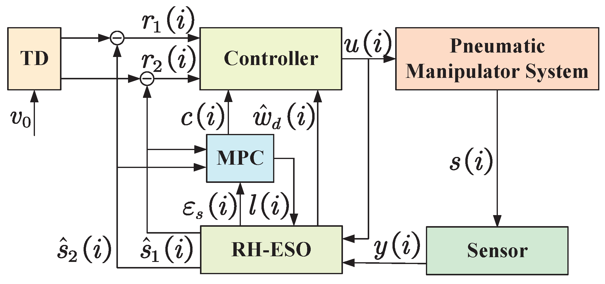
2.4. The MPC-Enabled Disturbance-Rejection Controller

To design the controller, the state tracking errors are denoted as $r_1\left(i\right)\triangleq v_1\left(i\right)-{\widehat{s}}_1\left(i\right)$ and $r_2\left(i\right)\triangleq v_2\left(i\right)-{\widehat{s}}_2\left(i\right)$. Then, the control input is designed as

$$\begin{array}{c}\hfill u\left(i\right)=k_1{r}_1\left(i\right)+k_2{r}_2\left(i\right)+c\left(i\right)-{\displaystyle \frac{1}{b_0}}{\widehat{s}}_3\left(i\right),\end{array}$$

(25)

where $k_1$ and $k_2$ are feedback gains to be designed; $c\left(i\right)$ is the decision variable of the MPC scheme to be obtained subsequently.

According to $r_1\left(i\right)$, $r_2\left(i\right)$, and (25), there exists

$$\begin{array}{cc}\hfill r_1(i+1)=& r_1\left(i\right)+\mathrm{T}{r}_2\left(i\right)-\mathrm{T}{\beta }_1{\epsilon }_1\left(i\right)-\mathrm{T}{l}_1\left(i\right),\hfill \\ \hfill r_2(i+1)=& r_2\left(i\right)-\mathrm{T}{b}_{0}u\left(i\right)+\mathrm{T}\mathrm{fhan}\left(i\right)-\mathrm{T}{b}_1{\widehat{s}}_1\left(i\right)-\mathrm{T}{\widehat{s}}_3\left(i\right)-\mathrm{T}{\beta }_2{\epsilon }_1\left(i\right)-\mathrm{T}{l}_2\left(i\right).\hfill \end{array}$$

Then, it is obtained that

$$\begin{array}{cc}\hfill r_1(i+1)=& r_1\left(i\right)+\mathrm{T}{r}_2\left(i\right)-\mathrm{T}{\beta }_1{\epsilon }_1\left(i\right)-\mathrm{T}{l}_1\left(i\right),\hfill \\ \hfill r_2(i+1)=& -\mathrm{T}{b}_0{k}_1{r}_1\left(i\right)+(1-\mathrm{T}{b}_0{k}_2)r_2\left(i\right)-\mathrm{T}{b}_{0}c\left(i\right)-\mathrm{T}{\beta }_2{\epsilon }_1\left(i\right)-\mathrm{T}{l}_2\left(i\right)+q\left(i\right),\hfill \end{array}$$

where $q\left(i\right)=\mathrm{T}\mathrm{fhan}\left(i\right)-\mathrm{T}{b}_1{\widehat{s}}_1\left(i\right)$.

Denote $r\left(i\right)\triangleq {\left[r_1\left(i\right)r_2\left(i\right)\right]}^T$. Then, it follows that

$$\begin{array}{c}\hfill r(i+1)=A_{r}r\left(i\right)+B_r{\epsilon }_s\left(i\right)+C_{r}c\left(i\right)+D_{r}l\left(i\right)+E_{r}q\left(i\right).\end{array}$$

where

$$\begin{gathered} A_r\triangleq \left[\begin{array}{cc}1& \mathrm{T}\\ -\mathrm{T}{b}_0{k}_1& 1-\mathrm{T}{b}_0{k}_2\end{array}\right],B_r\triangleq \left[\begin{array}{cc}-\mathrm{T}{\beta }_1& {\mathbf{0}}_{1\times 5}\\ -\mathrm{T}{\beta }_2& {\mathbf{0}}_{1\times 5}\end{array}\right], \\ {C}_r\triangleq \left[\begin{array}{c}0\\ -\mathrm{T}{b}_0\end{array}\right],D_r\triangleq \left[\begin{array}{ccc}-\mathrm{T}& 0& 0\\ 0& -\mathrm{T}& 0\end{array}\right],E_r\triangleq \left[\begin{array}{c}0\\ 1\end{array}\right]. \end{gathered}$$

Then, $r\left(i\right)$ is constrained by $r\left(i\right)\in \mathcal{R}\triangleq \{r\left(i\right):b_r^{T}r\left(i\right)\le h_r\}$, where

$$b_r\triangleq \left[\begin{array}{cccc}1& -1& 0& 0\\ 0& 0& 1& -1\end{array}\right],h_r\triangleq {\left[\begin{array}{cccc}{\overline{r}}_1& {\overline{r}}_1& {\overline{r}}_2& {\overline{r}}_2\end{array}\right]}^T,$$

with ${\overline{r}}_1$ and ${\overline{r}}_2$ being given positive constants. Then, the constraint on $q\left(i\right)$ is obtained as

$$\begin{array}{c}\hfill q\left(i\right)\in \mathcal{Q}\triangleq \{q\left(i\right):b_q^{T}q\left(i\right)\le \overline{q}\},\end{array}$$

with $\overline{q}\triangleq \mathrm{T}{r}_s+\mathrm{T}{b}_1({\overline{s}}_1+{\overline{r}}_1)$. Denote $\zeta \left(i\right)\triangleq {\left[r^T\left(i\right){\epsilon }_s^T\left(i\right)\right]}^T$ and $h\left(i\right)\triangleq {\left[c^T\left(i\right)l^T\left(i\right)\right]}^T$. Then, we have

$$\begin{array}{c}\hfill \zeta (i+1)=A_{\zeta }\zeta \left(i\right)+B_{\zeta }h\left(i\right)+C_{\zeta }{l}^{-}\left(i\right)+D_{\zeta }q\left(i\right),\end{array}$$

where

$$A_{\zeta }\triangleq \left[\begin{array}{cc}{A}_r& B_r\\ {\mathbf{0}}_{6\times 2}& A_{\epsilon }\end{array}\right],B_{\zeta }\triangleq \left[\begin{array}{cc}{C}_r& D_r\\ {\mathbf{0}}_{6\times 1}& B_{\epsilon }\end{array}\right],C_{\zeta }\triangleq \left[\begin{array}{c}{\mathbf{0}}_{2\times 6}\\ D_{\epsilon }\end{array}\right],D_{\zeta }\triangleq \left[\begin{array}{c}{E}_r\\ {\mathbf{0}}_{6\times 1}\end{array}\right].$$

The nominal system of $\zeta \left(i\right)$ is obtained as

$$\begin{array}{c}\hfill \overline{\zeta }(i+1)=A_{\zeta }\overline{\zeta }\left(i\right)+B_{\zeta }h\left(i\right)+C_{\zeta }{l}^{-}\left(i\right),\end{array}$$

where $\overline{\zeta }\left(i\right)\triangleq {\left[{\overline{r}}^T\left(i\right){\overline{\epsilon }}_s^T\left(i\right)\right]}^T$ with

$$\begin{array}{cc}\hfill \overline{r}(i+1)=& A_r\overline{r}\left(i\right)+B_r{\overline{\epsilon }}_s\left(i\right)+C_{r}c\left(i\right),\hfill \\ \hfill {\overline{\epsilon }}_s(i+1)=& A_{\epsilon }{\overline{\epsilon }}_s\left(i\right)+B_{\epsilon }l\left(i\right)+D_{\epsilon }{l}^{-}\left(i\right).\hfill \end{array}$$

Accordingly, the constraints on $\overline{\zeta }\left(i\right)$ and $h\left(i\right)$ are obtained as

$$\begin{array}{cc}\hfill \overline{\zeta }\left(i\right)& \in \mathcal{M}\triangleq \{\overline{\zeta }\left(i\right):b_{\zeta }^T\overline{\zeta }\left(i\right)\le h_{\zeta }\},\hfill \\ \hfill h\left(i\right)& \in \mathcal{N}\triangleq \{h\left(i\right):{\tilde{b}}_u^T\overline{\zeta }\left(i\right)+b_h^{T}h\left(i\right)\le h_h+h_q\left(i\right)\},\hfill \end{array}$$

respectively, where

$$\begin{gathered} b_{\zeta }\triangleq \left[\begin{array}{cc}{b}_r& 0\\ 0& b_{{\epsilon }_s}\end{array}\right],h_{\zeta }\triangleq \left[\begin{array}{c}{h}_r\\ h_{{\epsilon }_s}\end{array}\right],h_q\left(i\right)\triangleq \left[\begin{array}{c}{b}_u^T{\widehat{s}}_3\left(i\right)\\ {\mathbf{0}}_{6\times 1}\end{array}\right], \\ {\tilde{b}}_u\triangleq \left[\begin{array}{cc}{\left[k_1{k}_2\right]}^T{b}_u& {\mathbf{0}}_{2\times 6}\\ {\mathbf{0}}_{6\times 2}& {\mathbf{0}}_{6\times 6}\end{array}\right],b_h\triangleq \left[\begin{array}{cc}{b}_u& {\mathbf{0}}_{1\times 3}\\ {\mathbf{0}}_{1\times 1}& {\mathbf{0}}_{1\times 3}\end{array}\right],h_h\triangleq \left[\begin{array}{c}{h}_u\\ {\mathbf{0}}_{6\times 1}\end{array}\right]. \end{gathered}$$

2.5. The MPC Scheme

In this paper, the MPC scheme is proposed to deal with the state and input constraints of the pneumatic manipulator as well as generate a part of the control input signal. To establish the MPC scheme, a cost function is designed as

$$\begin{array}{cc}\hfill J(\widehat{\mathbf{l}}\left(i\right),\widehat{\mathbf{h}}\left(i\right))\triangleq & \sum _{s=0}^{T_s-1}\left(\parallel \widehat{\zeta }{(s,i)\parallel }_Q^2+{\parallel \widehat{h}(s,i)\parallel }_R^2\right)+{\parallel \widehat{\zeta }(T_s,i)\parallel }_P^2,\hfill \end{array}$$

where $\widehat{\zeta }(s,i)$ is the predictive state with $\widehat{\zeta }(0,i)=\overline{\zeta }\left(i\right)=\zeta \left(i\right)$; $\widehat{h}(s,i)$ is the predictive decision variable; $\widehat{\zeta }\left(i\right)\triangleq {[{\widehat{\zeta }}^T(0,i){\widehat{\zeta }}^T(1,i)\dots {\widehat{\zeta }}^T(T_s,i)]}^T$ is the predictive state sequence; $\widehat{\mathbf{h}}\left(i\right)\triangleq {[{\widehat{h}}^T(0,i){\widehat{h}}^T(1,i)\dots {\widehat{h}}^T(T_s-1,i)]}^T$ is the predictive decision variable sequence with $\widehat{h}(0,i)=h\left(i\right)$; Q and R denote the positive definite weighting matrices; $P>0$ represents the terminal penalty matrix requiring design. The predictive horizon is denoted by $T_s$.

Next, the optimization problem of the MPC scheme can be formulated as

Prob 1:

$$\begin{array}{c}\hfill ({\widehat{\mathbf{l}}}^{*}\left(i\right),{\widehat{\mathbf{h}}}^{*}\left(i\right))\triangleq arg\underset{\widehat{\mathbf{h}}\left(i\right)}{min}J(\widehat{\mathbf{l}}\left(i\right),\widehat{\mathbf{h}}\left(i\right))\end{array}$$

subject to

$$\begin{array}{cc}\hfill & \widehat{\zeta }(s+1,i)=A_{\zeta }\widehat{\zeta }(s,i)+B_{\zeta }\widehat{h}(s,i)+C_{\zeta }{\widehat{l}}^{-}(s,i)\hfill \end{array}$$

(26)

$$\begin{array}{cc}\hfill & b_{\zeta }^T\widehat{\zeta }(s,i)\le h_{\zeta }-\varphi (s,i),s\in \mathbb{Z}[0,T_s-1]\hfill \end{array}$$

(27)

$$\begin{array}{cc}\hfill & {\tilde{b}}_u^T\widehat{\zeta }(s,i)+b_h^T\widehat{h}(s,i)\le h_h+({\overline{w}}_d+h_{{\epsilon }_3}){\left[11{\mathbf{0}}_{1\times 6}\right]}^T-\chi (s,i),s\in \mathbb{Z}[0,T_s-1],\hfill \end{array}$$

(28)

$$\begin{array}{cc}\hfill & \widehat{\zeta }(T_s,i)\in {\zeta }_T(T_s,i),\hfill \end{array}$$

(29)

where

$$\begin{array}{cc}\hfill & \varphi (s,i)\triangleq \sum _{j=0}^{s-1}\underset{q(s-1-j,i)\in \mathcal{Q}}{max}{b}_{\zeta }^T{A}_{\zeta }^j{D}_{\zeta }{e}_{\zeta }(s-1-j,i),\hfill \\ \hfill & \chi (s,i)\triangleq \sum _{j=0}^{s-1}\underset{q(s-1-j,i)\in \mathcal{Q}}{max}{\tilde{b}}_u^T{A}_{\zeta }^j{D}_{\zeta }{e}_{\zeta }(s-1-j,i),\hfill \\ \hfill & e_{\zeta }(s+1,i)=A_{\zeta }{e}_{\zeta }(s,i)+D_{\zeta }q(s,i),\varphi (0,i)\triangleq {\mathbf{0}}_{10\times 1},\chi (0,i)\triangleq {\mathbf{0}}_{8\times 1},e_{\zeta }(0,i)={\mathbf{0}}_{4\times 1},\hfill \\ \hfill & {\zeta }_T(T_s,i)\triangleq \widehat{\zeta }(T_s,i)\cap \widehat{\mathcal{H}}(T_s,i),\widehat{\zeta }(T_s,i)\triangleq \{\widehat{\zeta }(T_s,i):b_{\zeta }^T\widehat{\zeta }(T_s,i)\le h_{\zeta }-\varphi (T_s,i)\},\hfill \\ \hfill & \widehat{\mathcal{H}}(T_s,i)\triangleq \{\widehat{\zeta }(T_s,i):{\tilde{b}}_u^T\widehat{\zeta }(T_s,i)\le h_h+({\overline{w}}_d+h_{{\epsilon }_3}){\left[11{\mathbf{0}}_{1\times 6}\right]}^T-\chi (T_s,i)\},\hfill \\ \hfill & {\widehat{\zeta }}^{*}\left(i\right)\triangleq {[{\widehat{\zeta }}^{*T}(0,i){\widehat{\zeta }}^{*T}(1,i)\dots {\widehat{\zeta }}^{*T}(T_s,i)]}^T,{\widehat{\mathbf{h}}}^{*}\left(i\right)\triangleq {[{\widehat{h}}^{*T}(0,i){\widehat{h}}^{*T}(1,i)\dots {\widehat{h}}^{*T}(T_s-1,i)]}^T,\hfill \\ \hfill & {\widehat{l}}^{-}(s,i)=\left\{\begin{array}{cc}{l}^{-}\left(i\right),& s=0\\ \left[\begin{array}{c}\left[\begin{array}{cc}{\mathbf{0}}_{3\times 1}& I_{3\times 3}\end{array}\right]\widehat{h}(0,i)\\ \left[\begin{array}{cc}{I}_{3\times 3}& {\mathbf{0}}_{3\times 3}\end{array}\right]l^{-}\left(i\right)\end{array}\right],& s=1\\ \left[\begin{array}{c}\left[\begin{array}{cc}{\mathbf{0}}_{3\times 1}& I_{3\times 3}\end{array}\right]\widehat{h}(s-1,i)\\ \left[\begin{array}{cc}{\mathbf{0}}_{3\times 1}& I_{3\times 3}\end{array}\right]\widehat{h}(s-2,i)\end{array}\right],& s\in \mathbb{Z}[2,T_s-1]\end{array}\right.\hfill \end{array}$$

Remark 3.

The optimality of the RH-ESO proposed in this paper is fundamentally different from that in [21]. In [21], the system under consideration includes a slowly time-varying disturbance in the state equations and Gaussian white noise in the output equations. It should be noted that the optimality in [21] is defined in terms of a minimum-variance performance index for estimating the states $s_1\left(i\right)$ and $s_2\left(i\right)$ and does not address an optimal estimate of the disturbance $w_d\left(i\right)$. By contrast, the focus of this paper is on the rolling optimization of the disturbance estimation error ${\epsilon }_s\left(i\right)$ to obtain the optimal estimate of the slowly varying disturbance $w_d\left(i\right)$ at the current instant. This “optimal” estimate is understood as the one that minimizes the system control performance index—that is, the quadratic tracking error of the system state.

The structure diagram of the pneumatic manipulator system is presented in Figure 1.

Definition 1

([31]). System (3) is said to be uniformly bounded if, for all ${\Xi }_1>0$, there exists a constant ${\Xi }_2\left({\Xi }_1\right)$ such that

$$\begin{array}{c}\hfill \parallel s\left(0\right)\parallel \le {\Xi }_1\Rightarrow \parallel s\left(i\right)\parallel \le {\Xi }_2\left({\Xi }_1\right),\end{array}$$

holds for all $s\left(0\right)\in {\mathbb{R}}^n$ and $i\in {\mathbb{Z}}_{\ge 0}$.

Following the above discussion, this paper aims to achieve the following two objectives: (1) establish sufficient conditions to ensure that the proposed MPC scheme is recursively feasible, and (2) establish easily verifiable sufficient conditions to ensure that system (3) under control input (25) is uniformly bounded.

3. Results

This section establishes the recursive feasibility of Prob 1 and provides rigorous Lyapunov-based stability guarantees for the closed-loop system.

Firstly, the following lemma is given to prove the feasibility of Prob 1.

Lemma 1.

If Prob 1 is feasible at time instant t, then there exists at least one feasible solution for Prob 1 at time instant $i+1$.

Proof. 

Denote candidate decision variable sequences $\tilde{\mathbf{h}}(i+1)$ and ${\tilde{\mathbf{l}}}^{-}(i+1)$ as

$$\begin{array}{cc}\hfill & \tilde{\mathbf{h}}(i+1)\hfill \\ \hfill \triangleq & {\left[\begin{array}{ccc}{\tilde{h}}^T(0,i+1)& \dots & {\tilde{h}}^T(T_s,i+1)\end{array}\right]}^T\hfill \\ \hfill =& {\left[\begin{array}{cccc}{\widehat{h}}^{T*}(1,i)& \dots & {\widehat{h}}^{T*}(T_s-1,i)& {\mathbf{0}}_{4\times 1}\end{array}\right]}^T,\hfill \\ \hfill & {\tilde{\mathbf{l}}}^{-}(i+1)\hfill \\ \hfill \triangleq & {\left[\begin{array}{ccc}{\tilde{l}}^{-T}(0,i+1)& \dots & {\tilde{l}}^{-T}(T_s,i+1)\end{array}\right]}^T\hfill \\ \hfill =& {\left[\begin{array}{cccc}{\widehat{l}}^{-T}(1,i)& \dots & {\widehat{l}}^{-T}(T_s-1,i)& {\mathbf{0}}_{3\times 1}\end{array}\right]}^T,\hfill \end{array}$$

where $\tilde{h}(s,i+1)$ is a candidate decision variable for $s\in \mathbb{Z}[0,T_s]$. ${\widehat{l}}^{-}(s,i+1)$ can be obtained from $\tilde{h}(s,i+1)$ for $s\in \mathbb{Z}[0,T_s]$. Then, we have

$$\begin{array}{cc}\hfill \widehat{\zeta }(0,i+1)=& A_{\zeta }\widehat{\zeta }(0,i)+B_{\zeta }{\widehat{h}}^{*}(0,i)+C_{\zeta }{\widehat{l}}^{-*}(0,i)+D_{\zeta }q\left(i\right).\hfill \end{array}$$

(30)

By considering the predictive dynamics of $\zeta (i+1)$ based on $\tilde{\mathbf{h}}(i+1)$, it follows that the corresponding state predictions can be derived from the system’s predictive dynamics:

$$\begin{array}{cc}\hfill & \tilde{\zeta }(s+1,i+1)=A_{\zeta }\tilde{\eta }(s,i+1)+B_{\zeta }\tilde{h}(s,i+1)+C_{\zeta }{\tilde{l}}^{-}(s,i+1)+D_{\zeta }q(s,i+1),\hfill \end{array}$$

(31)

where $\tilde{\zeta }(s+1,i+1)$ is the feasible state for $s\in \mathbb{Z}[0,T_s]$.

Combining (26), (30), and (31), it is obtained that

$$\begin{array}{c}\hfill \tilde{\zeta }(s,i+1)={\widehat{\zeta }}^{*}(s,i)+A_{\zeta }^{s-1}{D}_{\zeta }q\left(i\right).\end{array}$$

(32)

Denote $\tilde{\mathbf{l}}(i+1)\triangleq {\left[\begin{array}{ccc}{\tilde{\zeta }}^T(0,i+1)& \dots & {\tilde{\zeta }}^T(T_s,i+1)\end{array}\right]}^T$ as the feasible predictive state sequence.

In order to ensure the existence of at least one solution for Prob 1 at each subsequent time step $i+1$, it is necessary that the following conditions are satisfied:

$$\begin{array}{cc}\hfill & b_{\zeta }^T\tilde{\zeta }(s,i+1)\le h_{\zeta }-\varphi (s,i+1),s\in \mathbb{Z}[0,T_s],\hfill \end{array}$$

(33)

$$\begin{array}{cc}\hfill & {\tilde{b}}_u^T\tilde{\zeta }(s,i+1)+b_h^T\tilde{h}(s,i+1)\le h_h+({\overline{w}}_d+h_{{\epsilon }_3}){\left[11{\mathbf{0}}_{1\times 6}\right]}^T-\chi (s,i+1),s\in \mathbb{Z}[0,T_s-1],\hfill \end{array}$$

(34)

$$\begin{array}{cc}\hfill & \tilde{\zeta }(T_s,i+1)\in {\zeta }_T(T_s,i+1).\hfill \end{array}$$

(35)

In the following analysis, conditions (33)–(35) will be demonstrated one by one. To begin with, we first provide the proof for condition (33). Assuming that Prob 1 has a feasible solution at time instant t, it directly follows that constraint (27) will be satisfied, which in turn implies

$$\begin{array}{c}\hfill b_{\zeta }^T{\widehat{\zeta }}^{*}(s,i)\le h_{\zeta }-\varphi (s,i),\end{array}$$

(36)

for $s\in \mathbb{Z}[0,T_s-2]$. Based on (32) and (36), we have $b_{\zeta }^T(\tilde{\zeta }(s,i+1)-A_{\zeta }^s{D}_{\zeta }q\left(i\right))\le h_{\zeta }-\varphi (s,i)$, which yields

$$\begin{array}{cc}\hfill & b_{\zeta }^T\tilde{\zeta }(s,i+1)\hfill \\ \hfill & \le h_{\zeta }-\varphi (s,i)+b_{\zeta }^T{A}_{\zeta }^s{D}_{\zeta }q\left(i\right)\hfill \\ \hfill & =h_{\zeta }-\sum _{j=0}^{s-1}\underset{q(s-1-j,i)\in \mathcal{Q}}{max}{b}_{\zeta }^T{A}_{\zeta }^j{D}_{\zeta }q(s-1-j,i)+b_{\zeta }^T{A}_{\zeta }^s{D}_{\zeta }\left(q\left(i\right)-\underset{q(s-j,i)\in \mathcal{Q}}{max}q(s-j,i)\right)\hfill \\ \hfill & \le h_{\zeta }-\sum _{j=0}^{s-1}\underset{q(s-1-j,i)\in \mathcal{Q}}{max}{b}_{\zeta }^T{A}_{\zeta }^j{D}_{\zeta }q(s-1-j,i)\hfill \\ \hfill & =h_{\zeta }-\varphi (s,i+1),\hfill \end{array}$$

for $s\in \mathbb{Z}[0,T_s]$. Thus, condition (33) holds true for all s within the interval $\mathbb{Z}[0,T_s]$.

Next, the condition (34) is verified for the time instant $i+1$. By utilizing the sequences $\tilde{\mathbf{h}}(i+1)$ and ${\tilde{\mathbf{l}}}^{-}(i+1)$, we have $\tilde{h}(s,i+1)=\widehat{h}(s,i)$ and ${\tilde{l}}^{-}(s,i+1)={\widehat{l}}^{-}(s,i)$. Based on (28) and (32), it follows that

$$\begin{array}{cc}\hfill & {\tilde{b}}_u^T(\tilde{\zeta }(s,i+1)-A_{\zeta }^s{D}_{\zeta }q\left(i\right))+b_h^T\widehat{h}(s,i)\le h_h+({\overline{w}}_d+h_{{\epsilon }_3}){\left[11{\mathbf{0}}_{1\times 6}\right]}^T-\chi (s,i),\hfill \end{array}$$

which indicates

$$\begin{array}{cc}\hfill & {\tilde{b}}_u^T\tilde{\zeta }(s,i+1)+b_h^T\tilde{h}(s,i+1)\le h_h+({\overline{w}}_d+h_{{\epsilon }_3}){\left[11{\mathbf{0}}_{1\times 6}\right]}^T-\chi (s,i)+{\tilde{b}}_u^T{A}_{\zeta }^s{D}_{\zeta }q\left(i\right))\hfill \\ \hfill & =h_h+({\overline{w}}_d+h_{{\epsilon }_3}){\left[11{\mathbf{0}}_{1\times 6}\right]}^T-\sum _{j=0}^{s-1}\underset{q(s-1-j,i)\in \mathcal{Q}}{max}{\tilde{b}}_u^T{A}_{\zeta }^j{D}_{\zeta }q(s-1-j,i)\hfill \\ \hfill & +{\tilde{b}}_u^T{A}_{\zeta }^s{D}_{\zeta }\left(q\left(i\right)-\underset{q(s-j,i)\in \mathcal{Q}}{max}q(s-j,i)\right)\hfill \\ \hfill & \le h_h+({\overline{w}}_d+h_{{\epsilon }_3}){\left[11{\mathbf{0}}_{1\times 6}\right]}^T-\sum _{j=0}^{s-1}\underset{q(s-1-j,i)\in \mathcal{Q}}{max}{\tilde{b}}_u^T{A}_{\zeta }^j{D}_{\zeta }q(s-1-j,i)\hfill \\ \hfill & =h_h+({\overline{w}}_d+h_{{\epsilon }_3}){\left[11{\mathbf{0}}_{1\times 6}\right]}^T-\chi (s,i+1)\hfill \end{array}$$

for $s\in \mathbb{Z}[0,T_s-2]$. For $s=T_s-1$, there exist $\tilde{h}(T_s,i+1)={\mathbf{0}}_{4\times 1}$ and ${\tilde{l}}^{-}(T_s,i+1)={\mathbf{0}}_{6\times 1}$. Based on (29) and (32), $\tilde{h}(T_s,i+1)$ and ${\tilde{l}}^{-}(T_s,i+1)$, it is easy to obtain

$$\begin{array}{cc}\hfill & {\tilde{b}}_u^T(\tilde{\zeta }(T_s,i+1)-A_{\zeta }^{T_s-1}{D}_{\zeta }q\left(i\right))\le h_h+({\overline{w}}_d+h_{{\epsilon }_3}){\left[11{\mathbf{0}}_{1\times 6}\right]}^T-\chi (T_s,i),\hfill \end{array}$$

which means

$$\begin{array}{cc}\hfill & {\tilde{b}}_u^T\tilde{\zeta }(T_s,i+1)\le h_h+({\overline{w}}_d+h_{{\epsilon }_3}){\left[11{\mathbf{0}}_{1\times 6}\right]}^T-\chi (T_s,i)+{\tilde{b}}_u^T{A}_{\zeta }^{T_s-1}{D}_{\zeta }q\left(i\right)\hfill \\ \hfill =& h_h+({\overline{w}}_d+h_{{\epsilon }_3}){\left[11{\mathbf{0}}_{1\times 6}\right]}^T-\sum _{j=0}^{T_s-2}\underset{q(T_s-2-j,i)\in \mathcal{Q}}{max}{\tilde{b}}_u^T{A}_{\zeta }^j{D}_{\zeta }q(T_s-2-j,i)\hfill \\ \hfill & -{\tilde{b}}_u^T{A}_{\zeta }^{T_s-1}{D}_{\zeta }\underset{q(T_s-1-j,i)\in \mathcal{Q}}{max}q(T_s-1-j,i)+{\tilde{b}}_u^T{A}_{\zeta }^{T_s-1}{D}_{\zeta }q\left(i\right)\hfill \\ \hfill \le & h_h+({\overline{w}}_d+h_{{\epsilon }_3}){\left[11{\mathbf{0}}_{1\times 6}\right]}^T-\sum _{j=0}^{T_s-2}\underset{q(T_s-2-j,i)\in \mathcal{Q}}{max}{\tilde{b}}_u^T{A}_{\zeta }^j{D}_{\zeta }q(T_s-2-j,i)\hfill \\ \hfill =& h_h+({\overline{w}}_d+h_{{\epsilon }_3}){\left[11{\mathbf{0}}_{1\times 6}\right]}^T-\chi (T_s,i+1).\hfill \end{array}$$

Thus, condition (34) holds true for all s within the interval $\mathbb{Z}[0,T_s-1]$.

Finally, the satisfaction of condition (35) is established. Thus, ${\zeta }_T(T_s,i+1)\triangleq \widehat{\zeta }(T_s,i)\cap \widehat{\mathcal{H}}(T_s,i+1)$. From (33), it follows that $\tilde{\zeta }(T_s,i+1)$ belongs to the set $\widehat{\zeta }(T_s,i)$. Additionally, based on (29), it can be readily shown that $\tilde{\zeta }(T_s,i+1)$ also lies within $\widehat{\mathcal{H}}(T_s,i)$.

Therefore, since both membership conditions are satisfied, we conclude that $\tilde{\zeta }(T_s,i+1)\in {\zeta }_T(T_s,i+1)$ holds true, thereby ensuring the validity of condition (35). □

Theorem 1.

If there exist appropriate parameters $k_1$, $k_2$, ${\beta }_1$, ${\beta }_2$, ${\beta }_3$, and a positive definite matrix P, make the linear matrix inequality (LMI)

$$\begin{array}{c}\hfill A_{\zeta }^{T}P{A}_{\zeta }-P+Q<0,\end{array}$$

hold; then, ${\epsilon }_s\left(i\right)\triangleq {\left[e_{s_1}\left(i\right)e_{s_2}\left(i\right)\right]}^T$ is uniformly bounded under the control input (25) with $e_{s_1}\left(i\right)\triangleq v_1\left(i\right)-s_1\left(i\right)$ and $e_{s_2}\left(i\right)\triangleq v_2\left(i\right)-s_2\left(i\right)$. Moreover, the state ${\epsilon }_s\left(i\right)$ converges to the set $\mathcal{E}\triangleq \{{\epsilon }_s\left(i\right):\parallel {\epsilon }_s\left(i\right)\parallel \le \parallel M\parallel {\underline{\lambda }}^{-{\displaystyle \frac{1}{2}}}\left(Q\right){\sigma }^{{\displaystyle \frac{1}{2}}}\}$ with

$$\begin{array}{cc}\hfill \sigma \triangleq & 2{\overline{\lambda }}^2\left(P\right)\Theta \left(T_s\right)\Omega \left(T_s\right)+{\overline{\lambda }}^2\left(P\right){\Omega }^2\left(T_s\right)+\sum _{s=1}^{T_s-1}\left(2{\overline{\lambda }}^2\left(Q\right)\Theta \left(s\right)\Omega \left(s\right)+{\overline{\lambda }}^2\left(Q\right){\Omega }^2\left(s\right)\right)\hfill \\ \hfill \Theta \left(s\right)\triangleq & \underset{b_{\zeta }^T{\widehat{\zeta }}^{*}(s,i)\le h_{\zeta }-\varphi (s,i)}{max}\parallel {\widehat{\zeta }}^{*}(s,i)\parallel ,\hfill \\ \hfill \Omega \left(s\right)\triangleq & \underset{b_q^{T}q\left(i\right)\le \overline{q}}{max}\parallel A_{\zeta }^{s-1}{D}_{\zeta }q\left(i\right)\parallel ,\hfill \\ \hfill M\triangleq & \left[\begin{array}{ccccc}1& 0& -1& 0& 0\\ 0& 1& 0& -1& 0\end{array}\right].\hfill \end{array}$$

Proof. 

Considering $e_{s_1}\left(i\right)\triangleq r_1\left(i\right)-{\epsilon }_1\left(i\right)$ and $e_{s_2}\left(i\right)\triangleq r_2\left(i\right)-{\epsilon }_2\left(i\right)$, it can be obtained that $\parallel e_{s_1}\left(i\right)\parallel \le \parallel r_1\left(i\right)\parallel +\parallel {\epsilon }_1\left(i\right)\parallel$ and $\parallel e_{s_2}\left(i\right)\parallel \le \parallel r_2\left(i\right)\parallel +\parallel {\epsilon }_2\left(i\right)\parallel$. Subsequently, the proof of uniform boundedness of $\parallel e_{s_1}\left(i\right)\parallel$ and $\parallel e_{s_2}\left(i\right)\parallel$ is given first.

Denote the optimal cost of Prob 1 at time instant i as

$$\begin{array}{cc}\hfill J({\widehat{\mathbf{l}}}^{*}\left(i\right),{\widehat{\mathbf{h}}}^{*}\left(i\right))\triangleq & \sum _{s=0}^{T_s-1}\left(\parallel {\widehat{\zeta }}^{*}{(s,i)\parallel }_Q^2+{\parallel {\widehat{h}}^{*}(s,i)\parallel }_R^2\right)+{\parallel {\widehat{\zeta }}^{*}(T_s,i)\parallel }_P^2\hfill \end{array}$$

Then, a Lyapunov candidate function is denoted as $V\left(i\right)\triangleq J({\widehat{\mathbf{l}}}^{*}\left(i\right),{\widehat{\mathbf{h}}}^{*}\left(i\right))$. Consequently, there exists

$$\begin{array}{cc}\hfill \Delta V\left(i\right)\triangleq & J({\widehat{\mathbf{l}}}^{*}(i+1),{\widehat{\mathbf{h}}}^{*}(i+1))-J({\widehat{\mathbf{l}}}^{*}\left(i\right),{\widehat{\mathbf{h}}}^{*}\left(i\right))\hfill \end{array}$$

Given the optimal solution that Prob 1 is obtained at time instant i, then Prob 1 has at least one feasible solution at $i+1$ by Lemma 1. Therefore, the feasible cost of Prob 1 at time instant $i+1$ can be denoted as

$$\begin{array}{cc}\hfill & J(\tilde{\mathbf{l}}(i+1),\tilde{\mathbf{h}}(i+1))\triangleq \sum _{s=0}^{T_s-1}\left(\parallel \tilde{\zeta }{(s,i+1)\parallel }_Q^2+{\parallel \tilde{h}(s,i)\parallel }_R^2\right)+{\parallel \tilde{\zeta }(T_s,i+1)\parallel }_P^2\hfill \end{array}$$

Denote

$$\begin{array}{c}\hfill \Delta \tilde{V}\left(i\right)\triangleq J(\tilde{\mathbf{l}}(i+1),\tilde{\mathbf{h}}(i+1))-J({\widehat{\mathbf{l}}}^{*}\left(i\right),{\widehat{\mathbf{h}}}^{*}\left(i\right))\end{array}$$

Split $\Delta \tilde{V}\left(i\right)\triangleq {\Delta }_1\left(i\right)+{\Delta }_2\left(i\right)+{\Delta }_3\left(i\right)$, where

$$\begin{array}{cc}\hfill {\Delta }_1\left(i\right)\triangleq & \sum _{s=1}^{T_s-1}\left(\parallel \tilde{\zeta }{(s,i+1)\parallel }_Q^2-{\parallel {\widehat{\zeta }}^{*}(s,i)\parallel }_Q^2\right)+\sum _{s=1}^{T_s-1}\left(\parallel \tilde{h}{(s,i+1)\parallel }_R^2-{\parallel {\widehat{h}}^{*}(s,i)\parallel }_R^2\right)\hfill \\ \hfill {\Delta }_2\left(i\right)\triangleq & \parallel \tilde{\zeta }(T_s,i+1){\parallel }_Q^2+\parallel \tilde{h}(T_s,i+1){\parallel }_R^2+\parallel \tilde{\zeta }(T_s,i+1){\parallel }_P^2-{\parallel {\widehat{\zeta }}^{*}(T_s,i)\parallel }_P^2\hfill \\ \hfill {\Delta }_3\left(i\right)\triangleq & -\parallel {\widehat{\zeta }}^{*}{(0,i)\parallel }_Q^2-{\parallel {\widehat{h}}^{*}(0,i)\parallel }_R^2\hfill \end{array}$$

For ${\Delta }_1\left(i\right)$, there exists $\tilde{h}(s,i+1)={\widehat{h}}^{*}(s,i)$ for $s\in \mathbb{Z}[1,T_s-1]$. Therefore, it is obtained that

$$\begin{array}{cc}\hfill {\Delta }_1\left(i\right)& =\sum _{s=1}^{T_s-1}\left(\parallel {\widehat{\zeta }}^{*}(s,i)+A_{\zeta }^{s-1}{D}_{\zeta }{q\left(i\right)\parallel }_Q^2\right)-\sum _{s=1}^{T_s-1}\left(\parallel {\widehat{\zeta }}^{*}{(s,i)\parallel }_Q^2\right)\hfill \\ \hfill =& \sum _{s=1}^{T_s-1}\left(\parallel {\widehat{\zeta }}^{*}(s,i)+A_{\zeta }^{s-1}{D}_{\zeta }{q\left(i\right)\parallel }_Q+{\parallel {\widehat{\zeta }}^{*}(s,i)\parallel }_Q\right)\hfill \\ \hfill & \times \sum _{s=1}^{T_s-1}\left(\parallel {\widehat{\zeta }}^{*}(s,i)+A_{\zeta }^{s-1}{D}_{\zeta }{q\left(i\right)\parallel }_Q-{\parallel {\widehat{\zeta }}^{*}(s,i)\parallel }_Q\right)\hfill \\ \hfill \le & \sum _{s=1}^{T_s-1}\left(2\parallel {\widehat{\zeta }}^{*}{(s,i)\parallel }_Q+{\parallel A_{\zeta }^{s-1}{D}_{\zeta }q\left(i\right)\parallel }_Q\right){\parallel A_{\zeta }^{s-1}{D}_{\zeta }q\left(i\right)\parallel }_Q\hfill \\ \hfill \le & \sum _{s=1}^{T_s-1}\left(2{\overline{\lambda }}^2\left(Q\right)\Theta \left(s\right)\Omega \left(s\right)+{\overline{\lambda }}^2\left(Q\right){\Omega }^2\left(s\right)\right)\hfill \end{array}$$

where

$$\begin{array}{cc}\hfill \Theta \left(s\right)\triangleq & \underset{b_{\zeta }^T{\widehat{\zeta }}^{*}(s,i)\le h_{\zeta }-\varphi (s,i)}{max}\parallel {\widehat{\zeta }}^{*}(s,i)\parallel ,\Omega \left(s\right)\triangleq \underset{b_q^{T}q\left(i\right)\le \overline{q}}{max}\parallel A_{\zeta }^{s-1}{D}_{\zeta }q\left(i\right)\parallel \hfill \end{array}$$

For ${\Delta }_2\left(i\right)$, there exists $\tilde{h}(T_s,i+1)={\mathbf{0}}_{4\times 1}$. Then, it follows that

$$\begin{array}{cc}\hfill {\Delta }_2\left(i\right)& \triangleq \parallel \tilde{\zeta }(T_s,i+1){\parallel }_P^2-\parallel {\widehat{\zeta }}^{*}(T_s,i){\parallel }_P^2+\parallel \tilde{\zeta }(T_s,i+1){\parallel }_P^2-\parallel \tilde{\zeta }(T_s,i+1){\parallel }_P^2+{\parallel \tilde{\zeta }(T_s,i+1)\parallel }_Q^2\hfill \\ \hfill =& \parallel \tilde{\zeta }(T_s,i+1){\parallel }_P^2-\parallel {\widehat{\zeta }}^{*}(T_s,i){\parallel }_P^2-{\parallel \tilde{\zeta }(T_s,i+1)\parallel }_{\overline{Q}}^2\hfill \\ \hfill \le & \left(\parallel {\widehat{\zeta }}^{*}(T_s,i)+A_{\zeta }^{T_s-1}{D}_{\zeta }q\left(i\right){\parallel }_P+{\parallel {\widehat{\zeta }}^{*}(T_s,i)\parallel }_P\right)\times \parallel A_{\zeta }^{T_s-1}{D}_{\zeta }{q\left(i\right)\parallel }_P-{\parallel \tilde{\zeta }(T_s,i+1)\parallel }_{\overline{Q}}^2\hfill \\ \hfill \le & 2{\overline{\lambda }}^2\left(P\right)\Theta \left(T_s\right)\Omega \left(T_s\right)+{\overline{\lambda }}^2\left(P\right){\Omega }^2\left(T_s\right)-{\parallel \tilde{\zeta }(T_s,i+1)\parallel }_{\overline{Q}}^2\hfill \end{array}$$

where $\overline{Q}=P-Q-A_{\zeta }^{T}P{A}_{\zeta }$. If there exist appropriate parameters $k_1$, $k_2$, ${\beta }_1$, ${\beta }_2$, ${\beta }_3$, and a positive definite matrix P, make the LMI

$$\begin{array}{c}\hfill A_{\zeta }^{T}P{A}_{\zeta }-P+Q<0\end{array}$$

hold, and then $-\parallel \tilde{\zeta }(T_s,i+1){\parallel }_{\overline{Q}}^2\le 0$. In this case, it follows that

$$\begin{array}{cc}\hfill {\Delta }_2\left(i\right)\le & 2{\overline{\lambda }}^2\left(P\right)\Theta \left(T_s\right)\Omega \left(T_s\right)+{\overline{\lambda }}^2\left(P\right){\Omega }^2\left(T_s\right)\hfill \end{array}$$

For ${\Delta }_3\left(i\right)$, it yields ${\Delta }_3\left(i\right)\le -{\parallel {\widehat{\zeta }}^{*}(0,i)\parallel }_Q^2$.

Combining ${\Delta }_1\left(i\right)$, ${\Delta }_2\left(i\right)$, and ${\Delta }_3\left(i\right)$, we have

$$\begin{array}{cc}\hfill \tilde{\Delta }V\left(i\right)=& {\Delta }_1\left(i\right)+{\Delta }_2\left(i\right)+{\Delta }_3\left(i\right)\hfill \\ \hfill \le & -\parallel {\widehat{\zeta }}^{*}{(0,i)\parallel }_Q^2+2{\overline{\lambda }}^2\left(P\right)\Theta \left(T_s\right)\Omega \left(T_s\right)+{\overline{\lambda }}^2\left(P\right){\Omega }^2\left(T_s\right)\hfill \\ \hfill & +\sum _{s=1}^{T_s-1}\left(2{\overline{\lambda }}^2\left(Q\right)\Theta \left(s\right)\Omega \left(s\right)+{\overline{\lambda }}^2\left(Q\right){\Omega }^2\left(s\right)\right)\hfill \end{array}$$

According to the principle of optimality, the feasible cost is greater than the optimal cost, which indicates $\Delta V\left(i\right)\le \tilde{\Delta }V\left(i\right)$. Then, there exists

$$\begin{array}{cc}\hfill \Delta V\left(i\right)\le & -\parallel {\widehat{\zeta }}^{*}{(0,i)\parallel }_Q^2+2{\overline{\lambda }}^2\left(P\right)\Theta \left(T_s\right)\Omega \left(T_s\right)+{\overline{\lambda }}^2\left(P\right){\Omega }^2\left(T_s\right)\hfill \\ \hfill & +\sum _{s=1}^{T_s-1}\left(2{\overline{\lambda }}^2\left(Q\right)\Theta \left(s\right)\Omega \left(s\right)+{\overline{\lambda }}^2\left(Q\right){\Omega }^2\left(s\right)\right)\hfill \end{array}$$

Letting $V\left(i\right)<0$, it follows that

$$\begin{array}{cc}\hfill \parallel {\widehat{\zeta }}^{*}{(0,i)\parallel }_Q^2>& 2{\overline{\lambda }}^2\left(P\right)\Theta \left(T_s\right)\Omega \left(T_s\right)+{\overline{\lambda }}^2\left(P\right){\Omega }^2\left(T_s\right)+\sum _{s=1}^{T_s-1}\left(2{\overline{\lambda }}^2\left(Q\right)\Theta \left(s\right)\Omega \left(s\right)+{\overline{\lambda }}^2\left(Q\right){\Omega }^2\left(s\right)\right)\hfill \end{array}$$

It indicates that $\zeta \left(i\right)={\widehat{\zeta }}^{*}(0,i)$ will converge to the set $\tilde{\mathcal{E}}\triangleq {\{\zeta \left(i\right):\parallel \zeta \left(i\right)\parallel }_Q^2\le \sigma \}$ under $h^{*}(0,i)$ as $i\to +\infty$ with

$$\begin{array}{cc}\hfill \sigma \triangleq & 2{\overline{\lambda }}^2\left(P\right)\Theta \left(T_s\right)\Omega \left(T_s\right)+{\overline{\lambda }}^2\left(P\right){\Omega }^2\left(T_s\right)+\sum _{s=1}^{T_s-1}\left(2{\overline{\lambda }}^2\left(Q\right)\Theta \left(s\right)\Omega \left(s\right)+{\overline{\lambda }}^2\left(Q\right){\Omega }^2\left(s\right)\right)\hfill \end{array}$$

Next, the proof that ${\epsilon }_s\left(i\right)$ is uniformly bounded is given. It is easy to get ${\epsilon }_s\left(i\right)=M\zeta \left(i\right)$, where

$$\begin{array}{cc}\hfill M=& \left[\begin{array}{ccccc}1& 0& -1& 0& 0\\ 0& 1& 0& -1& 0\end{array}\right]\hfill \end{array}$$

Then, as $i\to +\infty$, there exists

$$\begin{array}{cc}\hfill \parallel e_x(+\infty )\parallel =& \parallel M\zeta (+\infty )\parallel \le \parallel M\parallel \parallel \zeta (+\infty )\parallel \le \overline{\sigma }\hfill \end{array}$$

with $\overline{\sigma }\triangleq \parallel M\parallel {\underline{\lambda }}^{-{\displaystyle \frac{1}{2}}}\left(Q\right){\sigma }^{{\displaystyle \frac{1}{2}}}$, which suggests that ${\epsilon }_s\left(i\right)$ will converge to the set

$$\begin{array}{c}\hfill \mathcal{E}\triangleq \{{\epsilon }_s\left(i\right):\parallel {\epsilon }_s\left(i\right)\parallel \le \parallel M\parallel {\underline{\lambda }}^{-{\displaystyle \frac{1}{2}}}\left(Q\right){\sigma }^{{\displaystyle \frac{1}{2}}}\}\end{array}$$

as $i\to +\infty$. That is, the tracking error ${\epsilon }_s\left(i\right)$ is uniformly bounded under the control input (25). This completes the proof. □

Remark 4.

The main advantages of the proposed methodology are twofold: (1) a novel RH-ESO that significantly enhances disturbance estimation accuracy is proposed. By reformulating the disturbance estimation error as prediction states and recursively solving a constrained optimization problem at each sampling instant, this innovative structure guarantees optimal observer gain selection with proven convergence properties. (2) The MPC-enabled disturbance-rejection controller is proposed with disturbance compensation, which enables the closed-loop system to simultaneously achieve prescribed optimal control performance and maintain active disturbance-rejection capabilities.

4. Numerical Example

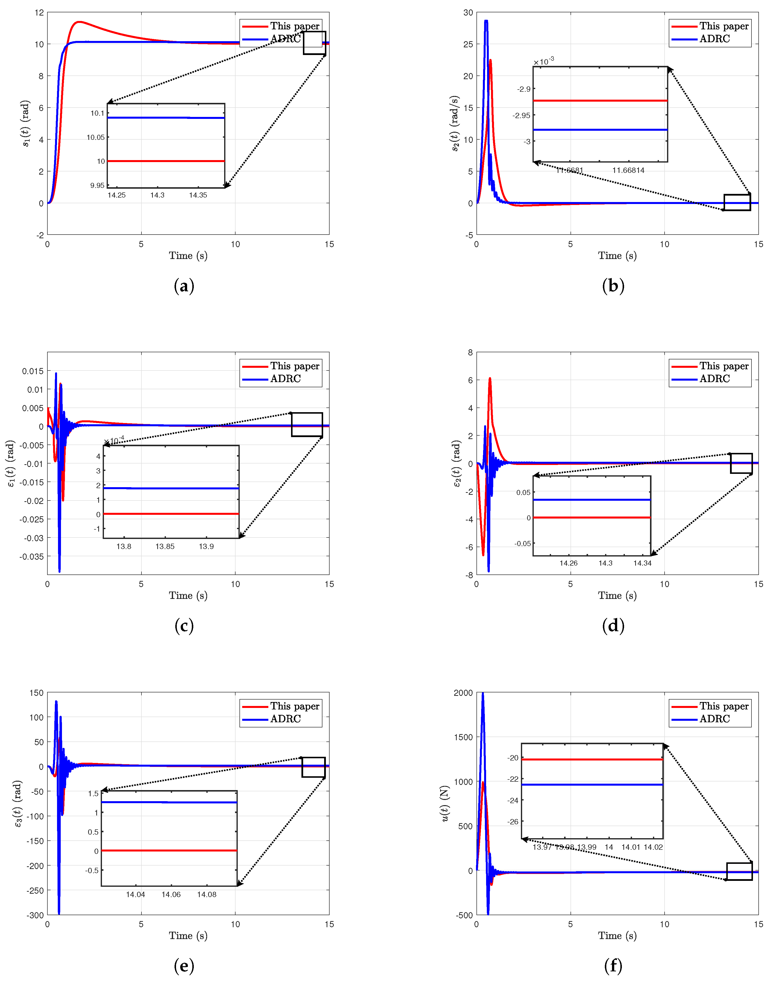
4.1. Time-Invariant Reference Input Signal Tracking

In this subsection, a numerical example of a pneumatic manipulator system is employed to validate the method and demonstrate its effectiveness. The simulation specifies an initial deflection angle of $0^{\circ }$ and a target deflection angle of ${10}^{\circ }$; i.e., $v_0\left(t\right)=10$. In this part, system (1) is used to demonstrate the effectiveness of the proposed method.

Parameters of the pneumatic manipulator system used in this subsection are presented in

Table 1. Parameters used in the simulation.

Parameter	$\tilde{R}$	$\tilde{l}$	$L_0$	b
Value	$0.1$ (m)	$0.3$ (m)	$0.3$ (m)	$0.3$ (m)
Parameter	$p_0$	m	g	$\mathrm{T}$
Value	1 (kpa)	1 (kg)	$9.8$ ($\mathrm{m}/{\mathrm{s}}^2$)	$0.01$ (s)
Parameter	$k_0$	N	${\overline{s}}_1$	${\overline{s}}_2$
Value	100	8	15	30
Parameter	$\overline{u}$	${\overline{\omega }}_d$	$h_{{\epsilon }_1}$	$h_{{\epsilon }_2}$
Value	1000	10	1	10
Parameter	$h_{{\epsilon }_3}$	${\beta }_1$	${\beta }_2$	${\beta }_3$
Value	100	300	7000	1750
Parameter	$k_1$	$k_2$	$r_1$	$r_2$
Value	100	30	20	50
Parameter	d	$T_s$	Q	R
Value	1	5	$I_{8\times 8}$	$0.5I_{4\times 4}$

.

In the following, the simulation results of the pneumatic manipulator system using the proposed MPC-enabled disturbance-rejection controller and the ADRC in Figure 2 are used to show the effectiveness of the proposed method in this paper.

Figure 2a plots the deflection angle $s_1\left(i\right)$ of the pneumatic manipulator system under the proposed MPC-enabled disturbance-rejection controller and the ADRC, respectively. From Figure 2a, it is evident that the proposed method can make the deflection angle closer to the set ${10}^{\circ }$. Figure 2b plots the angular velocity $s_2\left(i\right)$ of the pneumatic manipulator system.

Figure 2c–e plot the estimation errors ${\epsilon }_m\left(i\right)$ ($m=1,2,3$), respectively. It is evident that the proposed method achieves smaller estimation error magnitudes in steady-state conditions compared to the traditional ADRC approach. From Figure 2c–e, it is easy to find that the estimation errors under the proposed method demonstrate a smaller magnitude in steady-state conditions compared to that of the ADRC approach. Figure 2f plots the control input of the pneumatic manipulator system. In Figure 2f, it can be found that the proposed method effectively mitigates excessive control signal magnitudes, preventing potential actuator saturation and enhancing operational stability. As a result, from Figure 2a–f, the effectiveness of the proposed method is verified.

4.2. Time-Varying Reference Input Signal Tracking

In this subsection, the simulation specifies an initial deflection angle of $0^{\circ }$ and a time-varying target deflection angle of $v_0\left(t\right)=10sin(0.06\times 2\pi t+\pi /2)$. Furthermore, two simulation comparison groups are considered: (i) the back-stepping control (BSC) method described in [30], and (ii) a classical proportional–derivative (PD) controller. Note that system (37) is used in this subsection to demonstrate the effectiveness of the proposed method.

$$\begin{array}{c}\hfill \ddot{\theta }={\displaystyle \frac{\tilde{R}{k}_0}{2\pi N^{2}m{\tilde{l}}^2}}(3L_0^2-b^2)u-{\displaystyle \frac{3{\tilde{R}}^2{L}_0{p}_0}{\pi N^{2}m{\tilde{l}}^2}}\theta -{\displaystyle \frac{gsin\theta }{\tilde{l}}}+{\displaystyle \frac{3{\tilde{R}}^3{k}_0}{2\pi N^{2}m{\tilde{l}}^2}}{\theta }^{2}u+d+f,\end{array}$$

(37)

where $d=2sin{\displaystyle \frac{t}{20}}$ is an external disturbance term and $f=sin{\displaystyle \frac{\theta }{2}}$ is a model uncertainty term.

The parameters of the pneumatic manipulator system and the MPC scheme are the same as in Table 1. For given reference input signal $v_0\left(t\right)=10sin(0.06\times 2\pi t+\pi /2)$, the parameters of RH-ESO, ADRC, PD, and BSC are presented in

Table 2. Reference signal of $v_0\left(t\right)=10sin(0.06\times 2\pi t+\pi /2)$.

Parameters of RH-ESO and ADRC				${\mathit{\beta }}_1$	${\mathit{\beta }}_2$	${\mathit{\beta }}_3$	$k_1$	$k_2$
Value				150	550	100	70	10
Parameters of PD							$k_p$	$k_d$
Value							100	2
Parameters of BSC	${\xi }_1$	${\xi }_2$	${\xi }_3$	${\beta }_1$	${\beta }_2$	${\beta }_3$	$k_p$	$k_i$
Value	2	2	2	150	1000	100	50	$21.7$

, and the results are given in Figure 3.

Figure 3a plots the deflection angle of the pneumatic manipulator system (37). Figure 3b plots the deflection angle tracking error of the pneumatic manipulator system (37). Figure 3c plots the decision variables $l_m\left(t\right)$ ($m=1,2,3$) of the RH-ESO (9)–(11). Figure 3d plots the total costs throughout the entire simulation time of the pneumatic manipulator system (37) under the controller of this paper, ADRC, PD, and BSC, respectively. Note that the cost throughout the entire simulation time is calculated by the following formula:

$$\begin{array}{c}\hfill J\left(t\right)={\int }_0^t(\parallel s_1\left(\tau \right)-v_0{\left(\tau \right)\parallel }_Q^2+{\parallel u\left(\tau \right)\parallel }_R^2)d\tau \end{array}$$

where $t=50$, $Q=I$, and $R=0.01I$.

Under the same input signal, i.e., $v_0\left(t\right)=sin(0.06\times 2\pi t+\pi /2)$, the controller gain $k_1$ of the RH-ESO is increased from 70 to 130. The corresponding simulation results are shown in Figure 4.

Figure 4. Simulation results for reference signal $sin(0.06\times 2\pi t+\pi /2)$ of the pneumatic manipulator system using the parameters given in

Table 3. Reference signals of $v_0\left(t\right)=10sin(0.06\times 2\pi t+\pi /2)$.

Parameters of RH-ESO and ADRC				${\mathit{\beta }}_1$	${\mathit{\beta }}_2$	${\mathit{\beta }}_3$	$k_1$	$k_2$
Value				150	550	100	130	10
Parameters of PD							$k_p$	$k_d$
Value							100	2
Parameters of BSC	${\xi }_1$	${\xi }_2$	${\xi }_3$	${\beta }_1$	${\beta }_2$	${\beta }_3$	$k_p$	$k_i$
Value	2	2	2	150	1000	100	50	$21.7$

. (a) Deflection angle of the pneumatic manipulator system. (b) Deflection angle tracking error of the pneumatic manipulator system. (c) Decision variables of the RH-ESO. (d) Costs of the pneumatic manipulator system under these methods.

Figure 4. Simulation results for reference signal $sin(0.06\times 2\pi t+\pi /2)$ of the pneumatic manipulator system using the parameters given in Table 3. (a) Deflection angle of the pneumatic manipulator system. (b) Deflection angle tracking error of the pneumatic manipulator system. (c) Decision variables of the RH-ESO. (d) Costs of the pneumatic manipulator system under these methods.

From Figure 3a and Figure 4a, it can be clearly seen that the method mentioned in [30] exhibits overshoot and vibration phenomena in the early stages of simulation. The reason is that the control quantity fluctuates greatly. Nevertheless, during the early stage of state convergence, the system still experiences considerable overshoot accompanied by minor residual oscillations. This behavior is primarily attributable to the controller structure adopted in [30], which is given as

$$\begin{array}{cc}\hfill u\left(t\right)=& {\displaystyle \frac{-k_p{b}_1\left(t\right)s_1\left(t\right)-k_i\dot{e}\left(t\right)+{\alpha }_2\left(t\right)-{\int }_0^t({\xi }_3{\varsigma }_3\left(\tau \right)+{\varsigma }_2\left(\tau \right))d\tau +k_p{\ddot{\upsilon }}_1\left(t\right)}{k_p{b}_0}}-{\displaystyle \frac{{\widehat{s}}_3\left(t\right)}{b_0}}\hfill \end{array}$$

In this controller, an acceleration-level variable ${\ddot{v}}_1\left(t\right)$ and a velocity-level variable $\dot{e}\left(t\right)$ are employed. On the one hand, ${\ddot{v}}_1\left(t\right)$ is driven only by the reference signal, yet it exhibits large variations during the initial stage of the tracking differentiator, which seeks to follow the reference rapidly. On the other hand, the rate of change of $\dot{e}\left(t\right)$ in the control law $u\left(t\right)$ is much higher than that of $e\left(t\right)$. When $e\left(t\right)$ is large, $\dot{e}\left(t\right)$ oscillates frequently with considerable amplitude. These rapid oscillations further induce high-frequency large-magnitude oscillations in $u\left(t\right)$, leading to overshoot and oscillations in the state $s_1\left(t\right)$ at the outset. As $e\left(t\right)$ gradually converges, its amplitude diminishes, the amplitude of $\dot{e}\left(t\right)$ likewise decreases, and the oscillations in $u\left(t\right)$ become weaker and smaller. Consequently, during the subsequent tracking process, $s_1\left(t\right)$ no longer exhibits frequent oscillations or large excursions.

From Figure 3a and Figure 4a, it can be clearly seen that the estimated value ${\widehat{s}}_1\left(t\right)$ is oscillating during the simulation. The oscillations in the angle estimate ${\widehat{s}}_1\left(i\right)$ are directly caused by the decision vector $l^{*T}\left(i\right)={\left[l_1^{*T}\left(i\right)l_2^{*T}\left(i\right)l_3^{*T}\left(i\right)\right]}^T$. In the receding-horizon optimization problem proposed here, the variable to be optimized is defined as $h\left(i\right)\triangleq {\left[c^T\left(i\right)l^T\left(i\right)\right]}^T$. Because the receding-horizon strategy minimizes a cost that explicitly anticipates the evolution of states and decision variables over a future horizon, solving the optimization at time step i immediately yields the optimal decision vector $l^{*}\left(i\right)$. At the next instant, however, the optimal vector $l^{*}(i+1)$ is obtained by re-solving the problem with the updated initial state $\overline{\zeta }(i+1)\triangleq {\left[{\overline{r}}^T(i+1){\overline{\epsilon }}_s^T(i+1)\right]}^T$ and therefore bears no explicit relation to $l^{*}\left(i\right)$. Consequently, the value of $l^{*}\left(i\right)$ is determined solely by the optimization outcome. The oscillatory behavior of $l^{*}\left(i\right)$ thus corroborates the role of the receding-horizon mechanism: at each sampling instant, it predicts the state trajectory over the horizon from the current initial state and returns the decision vector that is optimal for that instant.

From Figure 3 and Figure 4, it can be seen that the proposed method achieves smoother bias angle tracking and the lowest overall control cost. Moreover, by comparing the simulation results, it is evident that the proposed method is insensitive to the controller gain $k_1$, whereas the traditional ADRC method is more sensitive to these gains. This further demonstrates the effectiveness of the proposed method.

4.3. Analysis of Estimation Error Under Different Observer Initial Values

In this subsection, we investigate the evolution of the estimation error when the RH-ESO initial states differ from that of the system. In

Table 4. Initial states of the system and the RH-ESO.

Initial states of the system	Variable	$s_1\left(0\right)$	$s_2\left(0\right)$
	Value	0	0
Case 1: Initial states of the RH-ESO	Variable	${\widehat{s}}_1\left(0\right)$	${\widehat{s}}_2\left(0\right)$
	Value	0	0
Case 2: Initial states of the RH-ESO	Variable	${\widehat{s}}_1\left(0\right)$	${\widehat{s}}_2\left(0\right)$
	Value	5	0
Case 3: Initial states of the RH-ESO	Variable	${\widehat{s}}_1\left(0\right)$	${\widehat{s}}_2\left(0\right)$
	Value	8	0

, three initial states of RH-ESO and the same initial value of the system are given.

Firstly, the case in which the reference signal is $v_0\left(t\right)=10$ is shown. The parameters of the proposed RH-ESO used in this case are those in Table 1. The corresponding results are given in Figure 5, Figure 6 and Figure 7.

From Figure 6 and Figure 7, it is easy to observe that there exist large values of the estimation errors ${\epsilon }_2\left(t\right)$ and ${\epsilon }_3\left(t\right)$. According to (12)–(14), when the same error signal ${\epsilon }_1\left(i\right)$ is used, the magnitudes of the terms ${\beta }_2{\epsilon }_1\left(i\right)$ and ${\beta }_3{\epsilon }_1\left(i\right)$ greatly exceed that of ${\beta }_1{\epsilon }_1\left(i\right)$. This results in relatively large values of ${\epsilon }_2\left(i\right)$ and ${\epsilon }_3\left(i\right)$ during the initial phase of the simulation. In addition, another simulation result can be obtained. From Figure 5, Figure 6 and Figure 7, it is easy to obtain that, the closer the initial value of the observer is to the reference signal, the higher the final observation accuracy when the reference is a constant signal.

Secondly, the case in which the reference signal is $v_0\left(t\right)=10sin(0.06\times 2\pi t+\pi /2)$ is shown. The parameters of the proposed RH-ESO in this case are those in Table 2.

The corresponding results are given in Figure 8, Figure 9 and Figure 10.

From Figure 9 and Figure 10, we can find that ${\epsilon }_2\left(t\right)$ and ${\epsilon }_3\left(t\right)$ remain relatively large at the beginning of the simulation. However, they are nevertheless much smaller than those obtained in Figure 6 and Figure 7. This reduction is due to a significant reduction in the RH-ESO gain used in sinusoidal tracking. Therefore, when the observation error shows a large value in the initial stage, the observer gain can be appropriately reduced to reduce the large value in the initial stage.

Furthermore, under these settings, the estimation accuracy is not as good as that achieved by a constant reference, and changing the initial state of the observer will not result in significant differences in the final observation error. The occurrence of this behavior is due to the fact that interference depends on time-varying states and control inputs, and the tracking of disturbance has a lag, resulting in a lag in the estimation of the system state. Therefore, the tracking error cannot converge precisely to zero but instead appears as a sine curve-like image. In general, a high observer gain effectively reduces the steady-state error; however, it also causes excessive overshoot at the beginning of the simulation. Therefore, the observer gain—high or low—should be selected flexibly according to the specific control requirements. In this simulation, the angle tracking error ultimately stays within ±0.05°, and the observation error during the initial phase is small and thus acceptable. Accordingly, the selected RH-ESO parameters are deemed appropriate.

5. Conclusions

This paper has proposed an MPC-enabled disturbance-rejection controller approach for a pneumatic manipulator system subjected to external disturbances. An RH-ESO has been designed that incorporates a decision variable to deal with the disturbances modeled from the complex nonlinear terms within the system. The optimal disturbance estimation error has been determined through a receding-horizon optimization procedure to obtain the best estimate of the disturbance. Using this optimal estimate, the MPC-enabled disturbance-rejection controller has been developed to enable precise angular trajectory tracking in the pneumatic manipulator system. Moreover, the recursive feasibility of Prob 1 has been guaranteed through rigorous proofs. Additionally, the uniform boundedness of the closed-loop system is mathematically guaranteed. Finally, the simulation results demonstrate the superior performance and effectiveness of the proposed approach.

References

1. Xie, Z.; Mohanakrishnan, M.; Wang, P.; Liu, J.; Xin, W.; Tang, Z.; Wen, L.; Laschi, C. Soft robotic arm with extensible stiffening layer. IEEE Robot. Autom. Lett. 2023, 8, 3597–3604. [Google Scholar] [CrossRef]
2. Low, J.H.; Lee, W.W.; Khin, P.M.; Thakor, N.V.; Kukreja, S.L.; Ren, H.L.; Yeow, C.H. Hybrid tele-manipulation system using a sensorized 3-D-printed soft robotic gripper and a soft fabric-based haptic glove. IEEE Robot. Autom. Lett. 2017, 2, 880–887. [Google Scholar] [CrossRef]
3. Yu, N.; Zhai, Y.; Yuan, Y.; Wang, Z. A bionic robot navigation algorithm based on cognitive mechanism of hippocampus. IEEE Trans. Autom. Sci. Eng. 2019, 16, 1640–1652. [Google Scholar] [CrossRef]
4. Chi, H.R.; Radwan, A.; Huang, N.F.; Tsang, K.F. Guest editorial: Next-generation network automation for industrial internet-of-things in Industry 5.0. IEEE Trans. Ind. Inform. 2022, 19, 2062–2064. [Google Scholar] [CrossRef]
5. Miron, G.; Plante, J.S. Design principles for improved fatigue life of high-strain pneumatic artificial muscles. Soft Robot. 2016, 3, 177–185. [Google Scholar] [CrossRef]
6. Kim, W.; Park, H.; Kim, J. Compact flat fabric pneumatic artificial muscle (ffpam) for soft wearable robotic devices. IEEE Robot. Autom. Lett. 2021, 6, 2603–2610. [Google Scholar] [CrossRef]
7. Tsai, T.C.; Chiang, M.H. A lower limb rehabilitation assistance training robot system driven by an innovative pneumatic artificial muscle system. Soft Robot. 2023, 10, 1–16. [Google Scholar] [CrossRef] [PubMed]
8. Cho, Y.; Kim, W.; Park, H.; Kim, J.; Na, Y. Bidirectional double-spring pneumatic artificial muscle with inductive self-sensing. IEEE Robot. Autom. Lett. 2023, 8, 8160–8167. [Google Scholar] [CrossRef]
9. Liu, G.; Diao, S.; Liu, Z.; Zhang, X.; Xiao, X.; Men, S.; Sun, N. Practical Finite-Time Compliant Control for Horizontal Pneumatic Artificial Muscle Systems Under Force-Sensorless Reflecting. IEEE Trans. Autom. Sci. Eng. 2024, 22, 9515–9527. [Google Scholar] [CrossRef]
10. Wang, Q.; Yang, T.; Liu, G.; Qin, Y.; Fang, Y.; Sun, N. Adaptive compensation tracking control for parallel robots actuated by pneumatic artificial muscles with error constraints. IEEE Trans. Ind. Inform. 2023, 20, 1585–1595. [Google Scholar] [CrossRef]
11. Liang, D.; Sun, N.; Wu, Y.; Liu, G.; Fang, Y. Fuzzy-sliding mode control for humanoid arm robots actuated by pneumatic artificial muscles with unidirectional inputs, saturations, and dead zones. IEEE Trans. Ind. Inform. 2021, 18, 3011–3021. [Google Scholar] [CrossRef]
12. Khaled, T.A.; Akhrif, O.; Bonev, I.A. Dynamic path correction of an industrial robot using a distance sensor and an ADRC controller. Ieee/Asme Trans. Mechatronics 2020, 26, 1646–1656. [Google Scholar] [CrossRef]
13. Diao, S.; Liu, G.; Liu, Z.; Zhou, L.; Sun, W.; Wang, Y.; Sun, N. Prescribed-Time Adaptive Fuzzy Control for Pneumatic Artificial Muscle-Actuated Parallel Robots With Input Constraints. IEEE Trans. Fuzzy Syst. 2023, 32, 2039–2051. [Google Scholar] [CrossRef]
14. Qin, Y.; Zhang, H.; Wang, X.; Sun, N.; Han, J. Adaptive set-membership filter based discrete sliding mode control for pneumatic artificial muscle systems with hardware experiments. IEEE Trans. Autom. Sci. Eng. 2023, 21, 1682–1694. [Google Scholar] [CrossRef]
15. Hosseini, S.A.; Toulabi, M.; Dobakhshari, A.S.; Ashouri-Zadeh, A.; Ranjbar, A.M. Delay compensation of demand response and adaptive disturbance rejection applied to power system frequency control. IEEE Trans. Power Syst. 2019, 35, 2037–2046. [Google Scholar] [CrossRef]
16. Zeng, Y.; Liang, G.; Liu, Q.; Rodriguez, E.; Pou, J.; Jie, H.; Liu, X.; Zhang, X.; Kotturu, J.; Gupta, A. Multiagent soft actor-critic aided active disturbance rejection control of DC solid-state transformer. IEEE Trans. Ind. Electron. 2024, 72, 492–503. [Google Scholar] [CrossRef]
17. Fu, C.; Tan, W. Tuning of linear ADRC with known plant information. ISA Trans. 2016, 65, 384–393. [Google Scholar] [CrossRef]
18. Guo, B.Z.; Zhao, Z.l. On the convergence of an extended state observer for nonlinear systems with uncertainty. Syst. Control Lett. 2011, 60, 420–430. [Google Scholar] [CrossRef]
19. Qin, B.; Yan, H.; Zhang, H.; Wang, Y.; Yang, S.X. Enhanced reduced-order extended state observer for motion control of differential driven mobile robot. IEEE Trans. Cybern. 2021, 53, 1299–1310. [Google Scholar] [CrossRef]
20. Li, Z.; Yan, H.; Zhang, H.; Yang, S.X.; Chen, M. Novel extended state observer design for uncertain nonlinear systems via refined dynamic event-triggered communication protocol. IEEE Trans. Cybern. 2022, 53, 1856–1867. [Google Scholar] [CrossRef]
21. Sun, H.; Madonski, R.; Li, S.; Zhang, Y.; Xue, W. Composite control design for systems with uncertainties and noise using combined extended state observer and Kalman filter. IEEE Trans. Ind. Electron. 2021, 69, 4119–4128. [Google Scholar] [CrossRef]
22. Zhao, L.; Li, Q.; Liu, B.; Cheng, H. Trajectory tracking control of a one degree of freedom manipulator based on a switched sliding mode controller with a novel extended state observer framework. IEEE Trans. Syst. Man Cybern. Syst. 2017, 49, 1110–1118. [Google Scholar] [CrossRef]
23. Zhao, L.; Cheng, H.; Wang, T. Sliding mode control for a two-joint coupling nonlinear system based on extended state observer. ISA Trans. 2018, 73, 130–140. [Google Scholar] [CrossRef]
24. Mayne, D.Q.; Rawlings, J.B.; Rao, C.V.; Scokaert, P.O. Survey constrained model predictive control: Stability and optimality. Automatica 2000, 36, 789–814. [Google Scholar] [CrossRef]
25. Zeilinger, M.N.; Morari, M.; Jones, C.N. Soft constrained model predictive control with robust stability guarantees. IEEE Trans. Autom. Control 2014, 59, 1190–1202. [Google Scholar] [CrossRef]
26. Li, T.; Sun, X.; Lei, G.; Guo, Y.; Yang, Z.; Zhu, J. Finite-control-set model predictive control of permanent magnet synchronous motor drive systems—An overview. IEEE/CAA J. Autom. Sin. 2022, 9, 2087–2105. [Google Scholar] [CrossRef]
27. Li, P.; Kang, Y.; Wang, T.; Zhao, Y.B. Disturbance prediction-based adaptive event-triggered model predictive control for perturbed nonlinear systems. IEEE Trans. Autom. Control 2022, 68, 2422–2429. [Google Scholar] [CrossRef]
28. Li, N.; Zhang, K.; Li, Z.; Srivastava, V.; Yin, X. Cloud-assisted nonlinear model predictive control for finite-duration tasks. IEEE Trans. Autom. Control 2022, 68, 5287–5300. [Google Scholar] [CrossRef]
29. Wang, M.; Cheng, P.; Zhang, Z.; Wang, M.; Chen, J. Periodic event-triggered MPC for continuous-time nonlinear systems with bounded disturbances. IEEE Trans. Autom. Control 2023, 68, 8036–8043. [Google Scholar] [CrossRef]
30. Zhao, L.; Li, Z.; Li, H.; Liu, B. Backstepping integral sliding mode control for pneumatic manipulators via adaptive extended state observers. ISA Trans. 2024, 144, 374–384. [Google Scholar] [CrossRef]
31. Peuteman, J.; Aeyels, D.; Sepulchre, R. Boundedness properties for time-varying nonlinear systems. SIAM J. Control Optim. 2001, 39, 1408–1422. [Google Scholar] [CrossRef]
Figure 1. Structure diagram of the pneumatic manipulator system.
Actuators 14 00343 g001
Figure 2. Simulation results for reference signal v 0 ( t ) = 10 of the pneumatic manipulator system. (a) The state s 1 ( i ) under the proposed method and the ADRC. (b) The state s 2 ( i ) under the proposed method and the ADRC. (c) The estimation error ε 1 ( i ) under the method in this paper and the ADRC. (d) The estimation error ε 2 ( i ) under the method in this paper and the ADRC. (e) The estimation error ε 3 ( i ) under the method in this paper and the ADRC. (f) The control input u ( i ) under the method in this paper and the ADRC.
Actuators 14 00343 g002
Figure 3. Simulation results for reference signal v 0 ( t ) = sin ( 0.06 × 2 π t + π / 2 ) of the pneumatic manipulator system using the parameters given in Table 2. (a) Deflection angle of the pneumatic manipulator system. (b) Deflection angle tracking error of the pneumatic manipulator system. (c) Decision variables of the RH-ESO. (d) Costs of the pneumatic manipulator system under these methods.
Actuators 14 00343 g003
Figure 5. The estimation error ε 1 ( t ) under different initial values of the proposed RH-ESO.
Actuators 14 00343 g005
Figure 6. The estimation error ε 2 ( t ) under different initial values of the proposed RH-ESO.
Actuators 14 00343 g006
Figure 7. The estimation error ε 3 ( t ) under different initial values of the proposed RH-ESO.
Actuators 14 00343 g007
Figure 8. The estimation error ε 1 ( t ) under different initial values of the proposed RH-ESO.
Actuators 14 00343 g008
Figure 9. The estimation error ε 2 ( t ) under different initial values of the proposed RH-ESO.
Actuators 14 00343 g009
Figure 10. The estimation error ε 3 ( t ) under different initial values of the proposed RH-ESO.
Actuators 14 00343 g010