Improved Static Model for Pneumatic Artificial Muscle Based on Virtual Work and Bladder Radial Deformation Work Losses

Abstract

Existing pneumatic artificial muscle (PAM) static geometrical models based on the principle of virtual work provide only approximate force predictions since they neglect the effects of volume change and radial bladder deformation work loss. In this study, we propose an improved geometrical static model called the Accurate Volume and Bladder Deformation Loss (AVBDL) model. This model introduces a physically consistent calculation of muscle volume at different contractions and pressures and incorporates a new way of describing work losses due to radial deformation of the bladder. The hyperelastic properties of the bladder were experimentally characterized and modeled using the Mooney–Rivlin formulation. The AVBDL model was validated against experimental data from four types of pneumatic muscles and compared with three established analytical models. Results show that the AVBDL model significantly improves force prediction accuracy, achieving a normalized root mean square (NRMS) error of 6.7–16.4%, compared to 20–68% for existing models. Due to its analytical transparency, reduced error, and broad applicability, the AVBDL model provides a robust basis for accurate simulation and control of pneumatic artificial muscles.

1. Introduction

Pneumatic artificial muscles (PAM) are lightweight mechanical actuators capable of producing large contractile forces when pressurized, as shown in Figure 1. The structure consists of an inner elastic bladder reinforced by a braided sleeve, which enables high power-to-weight ratios and inherent safety in human-interactive systems [1,2]. The specific nonlinear relationship between air pressure in the bladder, contraction, and generated force has long motivated research into accurate yet practical modeling techniques.

The first static PAM models were geometric or energy-based. Chou and Hannaford [3] derived the most known virtual work analytical model wherein they related pressure and contraction via braid geometry while assuming fibers did not extend. Tondu and Lopez [4] and Tsagarakis and Caldwell [5] upgraded this model by adding the effects of friction and radial pressure losses, which further improved its accuracy. Later Zhong et al. [6] integrated elastomer and braid elasticity using an Ogden strain/energy function, while Doumit and Leclair [7] proposed a stiffness-based correction model including cone-end deformation. Research work by Zhong et al. [6] and Doumit and Leclair [7] marked a shift from purely geometric models based only on braid geometry and contraction relationships toward analytical formulations that also incorporated the physical and material parameters of pneumatic artificial muscles.

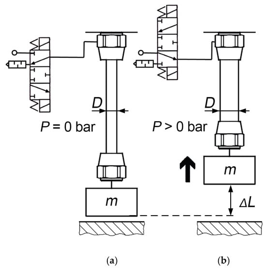
Figure 1. PAM before applying pressure (a) and after generating force and contraction with the increase in internal pressure, P (b) [8].

More recent studies have adopted existing mechanics or empirical extensions. Khajehsaeid and Soleymani [9] introduced a hyperelastic model based on limiting chain extensibility and network alteration theory, while Zang et al. [10] used exponential curve approximations for nonlinear fitting. Researchers also used phenomenological hysteresis models such as Prandtl–Ishlinskii [11] and Bouc–Wen [12] systems to model asymmetric behavior and later also hybrid approaches which combined analytical and neural models for enhanced prediction [13]. Although these methods improve accuracy, they require numerical optimization or data-driven training, reducing transparency and ease of use for these models.

Therefore, virtual-work analytical models remain the most widely applied because they are based on equations directly interpretable through physical quantities. This PAM model’s formulations do not include bladder radial deformation losses, which cause part of the pneumatic energy to dissipate during radial expansion rather than axial contraction, leading to lower-accuracy force prediction at higher pressures.

This study presents an improved analytical static model, the Accurate Volume and Bladder Deformation Loss (AVBDL) model, which was derived from the principle of virtual work and incorporating the measured material deformation of the bladder. This model introduces accurate volume calculations and radial deformation loss terms while still being based on an analytical and physics-based structure suitable for straightforward engineering implementation and control design.

2. PAM Bladder Deformation Analysis

The first step in developing the AVBDL model for predicting PAM force (we used the Festo DMSP-20 fluidic muscle (diameter 20 mm and length 200 mm), which differs from a conventional McKibben or general PAM in its reinforcing fibers, which are integrated within the bladder wall, whereas in traditional designs the fibers are woven externally around the bladder, but they behave and deform in same manner [8]) was to measure the bladder deformation during pressurization using a high-resolution camera system in order to precisely capture how the bladder shape changes under different pressures. Based on these observations, a geometric model of bladder deformation was developed as a function of internal pressure P and axial contraction ΔL, and the generated force was then calculated using the principle of virtual work.

In the second step, the material properties of the Festo DMSP-20 fluidic muscle bladder were determined through elastic deformation testing, followed by the development of a hyperelastic (Mooney–Rivlin) model describing its mechanical behavior.

Finally, both models were integrated into a unified analytical framework, and the predicted forces were compared with those obtained from Chou’s classical model and other established formulations, as well as with experimental data from this study and from other researchers.

For the geometrical modeling of the generated PAM force, the Chou and Hannaford model [14], which is based on virtual work, is most frequently used. The input work, dW_in, in the PAM is expressed as (1):

$$d{W}_{in}={\int }_{S_i}\left(P-P_0\right)d{l}_i d{s}_i=PdV$$

(1)

where P represents the absolute PAM pressure and P₀ the ambient pressure, dl_i represents the infinitesimal displacement of the inner surface element of the PAM bladder, ds_i denotes the corresponding area vector over which the pressure acts, P denotes the relative pressure, and dV represents the change in volume. If output work, W_out, (2), and input work, W_in, (1), are equal, we can calculate the force F as a function of the change in volume, which depends on the axial displacement, as shown by Equation (3).

$$d{W}_{out}=-F dL$$

(2)

$$F=-P {\displaystyle \frac{dV}{dL}}$$

(3)

where dW_out represents the output work, F the generated force, and dL the axial displacement. The Chou model then assumes the fiber length does not change and the generated force is calculated as a function of the change in fiber angle, as in (4).

$$F={\displaystyle \frac{\pi D_0^{2}P}{4}}\left(3 {cos\alpha }^{ 2}-1\right)$$

(4)

where D₀ is the initial PAM diameter, and α is the angle of fiber orientation. The change in volume is a function of the bladder shape and therefore we have to develop a model of it to calculate the volume and the change in volume.

2.1. Experimental Setup for PAM Volume and Force Measurement

To measure the bladder shape of the muscle, a high-resolution machine vision system was used. Machine vision applications are widely used in industry for fault detection, measurement, and data extraction [15]. The pneumatic muscle was mounted horizontally on linear guides using a precision clamping mechanism. It was axially fixed at several discrete positions, preventing axial contraction while the internal pressure was increased from 1 bar to 6 bar. This configuration was chosen to minimize hysteresis effects during measurement. Throughout the incremental pressurization, high-resolution images of the muscle were captured for subsequent deformation and volume analysis. The internal pressure was regulated by two fast-switching pneumatic valves, a pressure sensor, and an embedded PCX controller with a 16-bit analog input module, EL3104 (Figure 2, Table 1). Simultaneously, the generated axial force was continuously measured for later comparison with analytical model predictions.

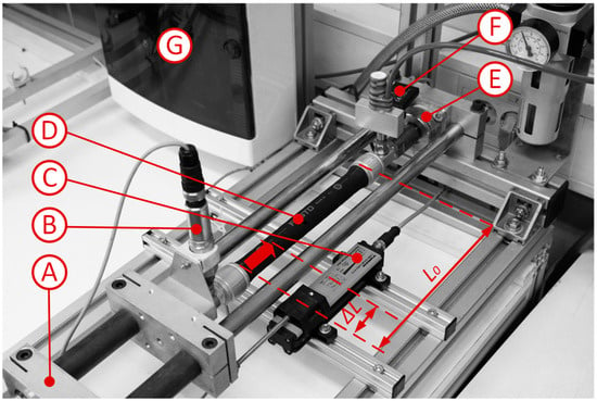
Figure 2. Image of pneumatic part of experimental setup. A—linear guides with clamping device; B—pressure sensor; C—displacement sensor; D—PAM Festo DMSP20 (Festo, Esslingen am Neckar, Germany); E—force sensor; F—fast switching valves; and G—PCX BECKHOFF CX 5000 controllers with I/O- modus (Beckhoff Automation, Verl, Germany). The pneumatic muscle has two connection ports; one is connected to the fast-switching valves for pressure control, and the opposite port is connected to the pressure sensor for direct measurement of internal pressure.

Table 1. Hardware used in experimental setup.

Name	Measurement Range	Measurement Accuracy	Output	Resolution
Pressure sensor FESTO SDET-22T (Festo, Esslingen am Neckar, Germany)	0–8 bar	0.1% FS	0–8 V	/
Force sensor VETEK TCPM 200 (Vetek, Väddö, Sweden)	0–2000 N	0.16% FS	1.5 mV/V	/
TURCK LI-Q25L (Turck, Mülheim an der Ruhr, Germany)	0–100 mm	0.025%	0–10 V	12 bit–0.025 mm
Camera acA2500-14gc (Basler, Ahrensburg, Germany)	/	/	GigE	2592 × 1944

The contractions (ΔL), which ranged from 0 mm to 30 mm, were measured for all pressure levels from 1 bar to 6 bar in steps of 2.5 mm, as shown in Table 2. During each pressure step, the PAM was fixed at these discrete contraction positions to record the corresponding deformation and volume changes. The final contraction value for each pressure level was measured without axial fixation, allowing the PAM to contract freely to its maximum displacement.

Table 2. Combinations of the measured parameters.

Pressure [bar]	1	2	3	4	5	6
ΔL [mm]	0–5	0–23	0–35	0–40	0–45	0–49

2.2. Modeling of PAM Bladder Shape

To determine the change in the PAM shape, the acquired images of all states of the PAM had to be prepared for further analysis. This was performed in 3 steps (Figure 3):

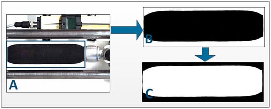
Figure 3. Image preparation for PAM deformation shape extraction. (A) Definition of a region of interest and cropping of the picture; (B) Conversion of the cropped picture from RGB to binary format, reduction of noise, and masking of the PAM logo; (C) Inversion of the picture for further blob analysis.

The next step was to determine the region of interest from the beginning of the muscle to the end of the deformed edge. The deformed edge shape was detected with the use of the edge detection function [16] (Figure 4) and then converted from pixels to mm.

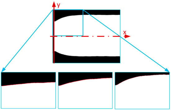
Figure 4. Image analysis of PAM deformation shape extraction [8].

To accurately define the change in the PAM edge, we had to fit the function to the experimental data. We completed this for every edge of every PAM contraction and pressure range. The function we were now looking for was the dependent y (the distance of the pneumatic bladder from the main axis) based on coordinate x, pressure P, and contraction ΔL, as presented in Equation (5).

$$y=f(x,P,\Delta L)$$

(5)

To fit the function, we tested 3 different function types: a polynomial function, multiple Gauss function superposition, and multiple Sine function superposition. After testing several candidate surface functions (including polynomial, multiple Gaussian, and multiple sine superposition forms), the best-fitting accuracy was achieved using the fourth-order polynomial function. This function demonstrated a coefficient of determination of approximately R = 0.97, outperforming the other tested forms both in terms of numerical accuracy and stability of fitted coefficients across different pressure and contraction conditions. The fourth-order polynomial provides sufficient flexibility to capture the nonlinear curvature of the PAM bladder edge while avoiding the oscillations and overfitting effects observed with higher-order or trigonometric approximations. Also, its analytical simplicity ensured easier integration into subsequent geometric and force modeling steps, maintaining a good balance between physical interpretability and computational efficiency. The most accurate function to fit the edge data appeared to be the 4th-order polynomial function shown in (6).

$$y\left(x,P,\Delta L\right)=p_4+p_3 x+p_2{ x}^2+p_1 x^3$$

(6)

The p₄ in (6) presents initial muscle radius, while p₁, p₂, and p₃ describe the shape of muscle’s deformed edge. The fourth-order polynomial function in Equation (6) was fitted to the experimentally extracted edge profiles of the PAM bladder, which were obtained from high-resolution camera images at different pressures and contraction levels. Each fitted curve represented the outer contour of the deformed bladder along the muscle length. We further fit function (6) to all extracted edge data and saved the coefficients p₁, p₂, p₃, and p₄. Then we had to determine whether the change in these coefficients depended on the pressure, P, or contraction, ΔL, as shown in (7).

$$p_n\left(P,\Delta L\right)=f\left(P,\Delta L\right)$$

(7)

We calculated that the coefficients did change. Therefore, we used Equation (8), which defines the dependence of these polynomial coefficients as a function of the internal pressure P and axial contraction ΔL, enabling interpolation of the bladder shape for any operating state.

$$p_n\left(P,\Delta L\right)=p_{0,3} {\Delta L}^3+p_{1,2} P {\Delta L}^2{+p}_{2,1}{P}^2 \Delta L+p_{0,2} {\Delta L}^2+p_{1,1} P \Delta L+p_{2,0}{P}^2+p_{0,1}\Delta L+p_{1,0}P+p_{0,0 }$$

(8)

All the coefficient values, from p_0,0 to p_1,2, were saved in the data matrix for the building of the final model. Figure 5 presents the results of the polynomial model fitted to experimental data for pressure p = 3 bar and different contractions. For better visibility, only every 15th element of the experimental data is shown. The experimental image analysis showed that the shape of the muscle changed only within the first 32 mm of its length. This was determined by measuring the edge profile from high-resolution camera images, which confirmed that, beyond 32 mm, the PAM contour remained straight with no observable deformations. Therefore, the polynomial function was fitted only in this area. The other part of the pneumatic muscle was not deformed but remained straight.

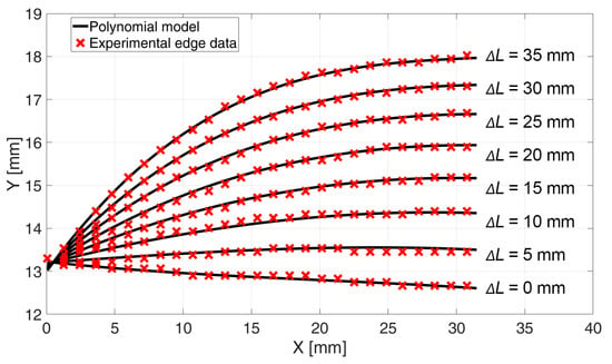
Figure 5. Fitted final polynomial model to experimental data at P = 3 bar and contraction of the PAM form ΔL = 0 mm to ΔL = 35 mm.

Through shape analysis, we obtained the shape of the PAM and with it the volume changes at static contraction under the influence of the internal pressure P. Changes in pressure P changed the volume of the muscle due to the elongation of internal fibers.

2.3. New Static Force Virtual Work Model

To calculate the generated force, we need to determine the volume of the muscle. This was performed by dividing the muscle into two areas, AR₁ and AR₂ (Figure 6). The first area, AR₁, represents the edge part which deforms and is always 32 mm wide for this type of PAM. The next area, AR₂, represents the straight part of the muscle and its length is a function of the muscle contraction.

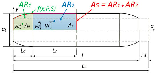
Figure 6. Two defined areas, AR₁ and AR₂, used for calculating the PAM volume. The x-axis represents the axial coordinate x along the muscle length, while the y-axis represents the radial deformation y(x,P,ΔL) of the bladder extracted from the polynomial fit. The deformed edge region (AR₁) is shown in green, and the straight region (AR₂) in blue, while As presents both areas combined.

To calculate the PAM volume, we used Guldin’s rule [17]. Equation (9) presents Guldin’s rule for volume calculation for the rotation of the area A_S.

$$V=2 \pi y_0 A_S$$

(9)

To calculate the volume, we must first calculate the area under the bladder polynomial function on the deformed and straight areas, as shown in (10).

$$y_0={\displaystyle \frac{y_d A_d+y_r A_r }{ A_d+A_r}}$$

(10)

We can calculate the center of gravity of the area under a function with (11). The integration limits in Equation (11) are a = 0 and b = L_d, corresponding to the active length of the deformed muscle, as shown explicitly in Equation (12). The center of gravity for y_d is then calculated with the use of (12), and for y_r with (13).

$$y={\displaystyle \frac{1}{A}}{\int }_a^b{\displaystyle \frac{1}{2}} {\left[f\left(x\right)\right]}^{2}dx$$

(11)

$$y_d={\displaystyle \frac{1}{2A_d}}{\int }_0^{L_d}{\left[f(x,P,\Delta L)\right]}^{2}dx$$

(12)

$$y_r={\displaystyle \frac{f\left({P,\Delta L,L}_d\right)}{2}}$$

(13)

The area under the deformed PAM edge is defined in (14), and the volume under the non-deformed part in (15).

$$A_d=-{\int }_0^{L_d}f(x,P,\Delta L)dx$$

(14)

$$A_r=f\left(L_d,P,\Delta L\right) {\displaystyle \frac{L_0-{2 L}_d-\Delta L}{2}}$$

(15)

Since A_S = A_d + A_r, the volume is therefore calculated as shown in (16) and (17).

$$V=4 \pi (y_d A_d+y_r A_r)$$

(16)

$$V=4 \pi \left(A+B \right)$$

(17)

To calculate the generated force, we combine (3) and (17) and generate the final (18), where ${A= y}_d A_d$ and ${B=y}_r A_r$. And since $\Delta L=Lo-\Delta L means dL= -d\Delta L$.

$$F=-\acute{P} {\displaystyle \frac{dV}{d\Delta L}}=-4 \pi \acute{P}\left({\displaystyle \frac{dA}{d\Delta L}}+{\displaystyle \frac{dB}{d\Delta L}} \right)$$

(18)

2.4. PAM Bladder Deformation Work

To calculate how much work is lost in the PAM bladder radial deformation, we must extract a radial part of the DMSP20 PAM and perform an axial stress test. In theory, the work used for bladder radial deformation reduces the output work and therefore generates the PAM force, as shown in (19), where W_ob represents the work used for bladder radial deformation.

$$W_{out}=W_{in}-W_{ob}$$

(19)

An axial test was performed on the extracted part of the PAM bladder, which was cut vertically to the PAM axis. The fibers in the PAM bladder stayed intact so that we could capture the effect of the internal friction between the fibers and rubber and also achieve as accurate a model as possible. The dimensions of the cut-out part were as follows: the length is 50 mm and the width is 13 mm. The maximum elongation was approximately 100% of the original length. As the test was also observed and analyzed with the use of machine vision, we were able to measure the change in the tested material width. In this way, we could calculate the real strain, taking into account the generated axial force at different elongations and also the change in the cross-section of the area.

Because the PAM bladder is a combination of rubber and reinforcement fibers, its material has the characteristic of being superelastic, and the most suitable model is therefore Mooney–Rivlin’s model [18,19]. This is because the coefficients can be calculated using Matlab curve fitting tool (version R2024b), and also integration of Mooney–Rivlin’s model for calculating deformation work does not present a problem. Since rubber is defined as uncompressible [20], its material properties can be defined using only uniaxial tensile stress. The Mooney–Rivlin’s model for this material is shown in (20).

$$\sigma =2 C_{10}\left(\lambda -{\displaystyle \frac{1}{{\lambda }^2}}\right)+2 C_{01}\left(\lambda -{\displaystyle \frac{1}{{\lambda }^3}}\right)+4 C_{20}\left(\lambda -{\displaystyle \frac{1}{{\lambda }^2}}\right)\left({\lambda }^2+{\displaystyle \frac{2}{\lambda }}-3\right)$$

(20)

The denotations C₁₀, C₀₁, and C₂₀ are the model coefficients and are calculated with the use of the Matlab curve fitting toolbox, and the symbol $\lambda$ represents the stretch ratio. Figure 7 represents the experimentally gathered stretch ratio vs. the tension data and is compared to the fitted Mooney–Rivlin’s model. The work performed by the deformation of the superelastic material is presented in (21) [18] and its integral in (22).

$$W_{def}=\underset{1}{\overset{\lambda }{\int }}\sigma \left(\lambda \right)d\lambda$$

(21)

$$W_{def}={\displaystyle \frac{ {\left(\lambda -1\right)}^2 }{{\lambda }^2}} \left(C_{01}+2 C_{01} \lambda +\left(2+\lambda \right) \left(C_{10} \lambda +C_{20} \left(2-3\lambda +{\lambda }^3\right)\right)\right)$$

(22)

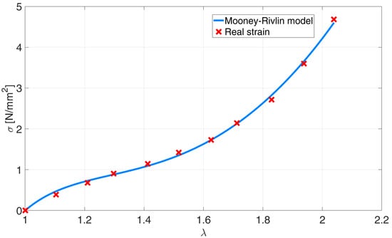
Figure 7. Mooney–Rivlin model fitted to the experimental data of the PAM bladder.

As the relation between stress and strain is nonlinear, the deformation of the entire muscle must not be calculated as an average deformation. Therefore, we again divided the muscle into two parts, AR1 and AR2, and calculated the deformation work for each of them, as shown in Figure 8.

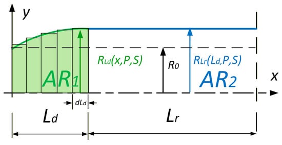
Figure 8. Two regions of the pneumatic artificial muscle (PAM) used for radial deformation work calculation. The x-axis represents the axial coordinate x along the muscle length, and the y-axis represents the instantaneous muscle radius R(x,P,ΔL). The deformed edge region (AR₁) and the straight region (AR₂) are indicated separately.

To calculate the work performed, we used a numerical method, and we used (23) to calculate the stretch ratio from the change in the PAM radius.

$$\lambda =R/R_0$$

(23)

where $\lambda$ is the ratio, R is the change in radius of the PAM, and R₀ is the starting radius of the PAM. Because the PAM radius, R_Ld, (Figure 9) along the deformed edge (part AR₁) changes differently than the PAM radius, R_Lr, it is considered in the calculation of the deformation work, W_def, which depends on both of them, as shown by (24).

$$W_{def}=V_{bl\left(Ld\right)} \sum _{x=0}^{Ld}{W}_{def}\left(R_{Ld}\right)+{V_{bl\left(Lr\right)} W}_{def}\left(R_{Lr}\right)$$

(24)

where V_bl is the PAM bladder volume, R is the change in radius of the PAM, and R₀ is the starting radius of the PAM. The final AVBDL model of PAM-generated force is presented in (25). It is based on an accurate virtual work model in combination with the calculations used to determine bladder radial deformation-related work loss.

$$F=-\acute{P} {\displaystyle \frac{dV}{d\Delta L}}+{\displaystyle \frac{W_{def}}{\Delta L}}$$

(25)

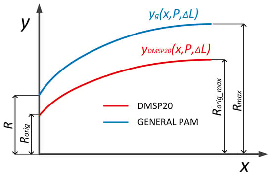
Figure 9. PAM shape generalization based on DMSP20 edge deformation. The x-axis corresponds to the normalized axial position along the muscle length, and the y-axis indicates the radial deformation y_g(x,P,ΔL) in mm. The figure illustrates how the generalized polynomial parameters reproduce the muscle contour for various pressures and contractions [8].

2.5. AVBDL Model Generalization

In order to use the new model for different muscles (different diameters, lengths, and bladder materials), the model was generalized. The first step was to geometrically define different muscle shapes depending on their diameter D, initial length L, and maximal contracted length L_min. This generalization was performed with Equation (6) and with this, the polynomial equation could describe the edge shape of any muscle. The maximal diameter was calculated with (26), which takes into account which area of the muscle does not change.

$$D_{max}={\displaystyle \frac{D_{\mathrm{o}} L_{\mathrm{o}}}{L_{min}}}$$

(26)

In (26), D₀ is muscle initial diameter, D_max is maximal muscle diameter, L₀ is general muscle length, and L_min is general muscle length at full contraction. Equation (6) was further generalized using the muscle’s initial and maximal diameters to describe the edge shape of any pneumatic muscle. The variable y_g represents the generalized radial deformation function of the pneumatic muscle edge, which defines the outer contour of the muscle as a function of the axial coordinate x, internal pressure P, and PAM contraction ΔL. This generalization allows the model to be applied to muscles of different sizes and geometries, as shown in Figure 9. The final form is presented in Equations (27)–(29).

$$y_g\left(x,P,\Delta L\right)=\left(p_4\left(P,\Delta L\right)+p_3\left(P,\Delta L\right) x+p_2\left(P,\Delta L\right){ x}^2+p_1\left(P,\Delta L\right) x^3\right) K_1+K_2$$

(27)

$$K_1={\displaystyle \frac{D_{F20\_max}-D_{F20}}{D_{max}-D}}$$

(28)

$$K_2=D-{\displaystyle \frac{320}{D_{max}-D}}$$

(29)

D_F20 = 20 mm is the diameter, D_{F20_max} = 36 mm is maximal muscle diameter at full contraction, and L_F20 = 200 mm is the length of the tested DMSP20 muscle (Festo, Esslingen am Neckar, Germany). Since the coefficients K₁ and K₂ do not change regarding pressure P and contraction ΔL, the volume (16) and generated force are calculated as in (18). The generalized muscle model was still divided into a deformed edge and an only radially deformed middle area. The dimension L_S = 32 mm and L_R were calculated from initial muscle length L.

The second step was calculation of work used for bladder radial contraction. This was performed through fitting Mooney–Rivlin’s hyperplastic model (20), to tensile test experimental data of the material used for the muscle bladder. The new hyperplastic model was then implemented in the final force model (25).

2.6. PAM Modeling Data

The next step in our research was to compare our AVBDL model to Chou’s and other geometrical static models and to the experimental results to validate the model and to evaluate it. To calculate the force from Chou’s model (4), we had to determine the angle of fibers in the PAM bladder, the PAM diameter, and the nominal PAM length. As there was no data about fiber orientation in the technical documentation for DMSP muscles, we therefore had to take apart one PAM to extract the required data. This proved that we could not use a model of friction between fibers to calculate the internal bladder losses. Figure 10 shows the photo of the original form of the PAM (A) and the photo without the bladder, where the fiber angle α is marked (B).

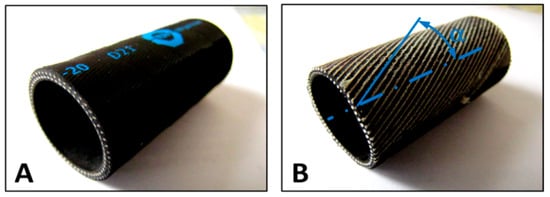
Figure 10. (A) Extracted PAM section used for determining the fiber orientation. (B) Ground outer layer showing fiber angle α relative to the muscle axis. The x-axis shows the longitudinal coordinate along the muscle, and the y-axis shows the fiber alignment angle measured by machine vision.

To extract data about the PAM fiber angle α, we used machine vision to detect lines from the image and to calculate the angle of fibers in relation to the PAM’s central axis. The dimensions of muscle DMSP20 needed for Chou’s model were the internal diameter of the PAM, D = 20 mm; the initial PAM length, L = 200 mm; the fiber length, L_S = 221 mm; the number of fibers turns, n = 1.5; and the fiber angle, α = 25°.

For model verification, we used experimental data gathered from two papers [21,22] which used different types of muscles. We also used experimental tests on the muscle made by Shadow Robot Company [23]. The dimensions and bladder materials of all three muscles used for model validation are presented in Table 3.

Table 3. Additional researched PAMs’ dimensions and materials.

Author	Davis Steven et al. [21]	Zuglian Ferrari et al. [22]	Shadow Robot Company [23]
D [mm]	30	15	30
L [mm]	470	465	200
n	4.7	3.2	1.9
Cont. [%]	31	20	37
Bladder material	Polyiso-butylene	Silicon rubber	Polyiso-butylene

Experimental tensile test results for polyisobutylene [22] and silicon rubber [22] were obtained with Matlab grabit toolbox and used to fit Mooney–Rivlin’s model.

3. Results

The new AVBDL model was first compared to the experimental data and Chou’s model. All the experimental data for the generated axial force of the PAM were obtained during the machine vision test.

The comparison between the new AVBDL model for muscle DMSP20, which considered work losses due to PAM bladder radial deformation, Chou’s model, and the experimental results is given in Figure 11. It is observed that the new AVBDL model with losses included very accurately defined the generated force as a function of pressure and contraction of the PAM, which was confirmed by the experimental results. The NRMS error of the AVBDL model was 4.6% and Chou’s model’s error was 21%.

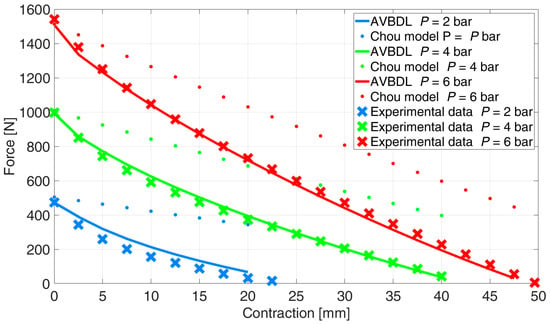
Figure 11. Comparison of the new AVBDL model with bladder deformation loss, Chou’s model, and experimental data.

The difference between the newly developed model and the experimental data was smaller at higher pressures. This was due to the effect of the internal bladder friction losses at lower pressures, where the internal friction has greater relative influence on the generated force and is also directly related to the hysteresis effect, as was proven by larger hysteresis loops at lower pressures [24].

The comparison of the generalized AVBDL static force model with Chou’s model was also performed for three different muscles with different structures and dimensions. With this test the general use of the AVBDL model for different pneumatic muscle actuators was tested. Figure 12 presents the experimental results of Davis S. et al.’s muscle [21], the AVBDL, and Chou’s geometrical model.

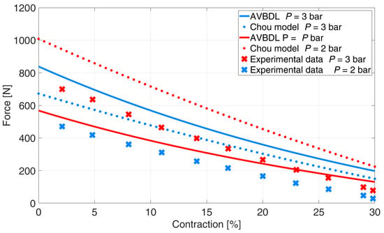
Figure 12. Comparison of generalized AVBDL model and experimental data for Davis S. et al.’s muscle [21].

The NRMS error at pressures p = 2 and 3 bar for Chou’s model was 35.2% and 9.9% for the AVBDL model. The comparison of the AVBDL model on Zuglian Ferrari et al.’s [22] muscle is presented in Figure 13. Chou’s model’s NRMS error for this muscle was 16.4%. The AVBDL model NRMS error was 38.8%.

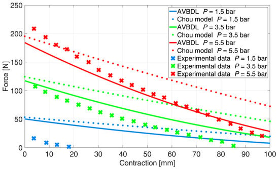
Figure 13. Comparison of generalized AVBDL model and experimental data for Zuglian Ferrari muscle [22].

The larger NRMS errors of Chou’s and the AVBDL model were due to the muscle being relatively long with a small diameter and thick muscle tubing of 5 mm. Also, the braiding used for this muscle was very thick, which resulted in complex friction and interlocking between fibers and resulted in increased model error at lower pressures under p = 1.5 bar.

The last validation was performed with Shadow Robot Company’s 30 mm muscle (Figure 14). The muscle was tested on our equipment at pressures p = 1, 2, and 3 bar since the maximal allowed muscle pressure was 3.5 bar. The NRMS error of Chou’s model was 25.7% and for the AVBDL model it was 11.7%.

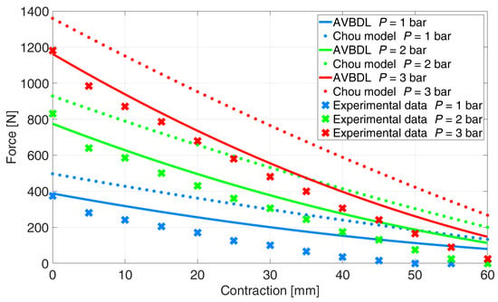
Figure 14. Comparison of generalized AVBDL model and experimental data for Shadow Robot Company muscle [23].

Table 4 presents a comparison between the proposed AVBDL model and several established geometrical models (Chou’s [3], K. Zang et al. [10], and M. Doumit et al. [25]). It can be clearly seen that the AVBDL model consistently provides the lowest NRMS error (6.7–16.4%), whereas the Chou and Hannaford models and other analytical models exhibit considerably higher errors of up to 68%. This improvement arises from two key features of the AVBDL formulation:

Table 4. Pneumatic muscle dimensions and materials.

Model	AVBDL	Chou and Hannaford (Geometrical Model) [3]	Kejiang Zang et al. [10]	Marc Doumit et al. [7]
Muscles tested	4 types	4 types	1 type	1 type
NRMS error	6.7–16.4%	20–38%	68%	49%

i

It introduces a more accurate geometric representation of the muscle by dividing it into the deformed and undeformed regions;

ii

It accounts for the radial deformation work losses of the bladder using experimentally identified Mooney–Rivlin parameters. These elements allow the model to reproduce the nonlinear force–pressure–contraction relationship more faithfully than previous purely geometric approaches.

Still, a certain deviation exists, mainly at lower pressures, due to friction between the inner fibers and the rubber bladder as well as local hysteresis effects that were not included in the current static formulation. Incorporating these losses through a pressure- and strain-dependent friction term, together with dynamic hysteresis modeling, could further reduce the residual error and expand the model’s applicability to cyclic and transient operation. Overall, the AVBDL model demonstrates both physical transparency and improved quantitative accuracy, making it a robust foundation for advanced control and simulation of pneumatic artificial muscles.

4. Discussion and Conclusions

The proposed AVBDL approach offers several advantages over existing pneumatic artificial muscle (PAM) static geometrical models. By integrating both geometric and material aspects of the muscle, it provides a physically interpretable framework with higher predictive accuracy across different PAM types. The model remains mathematically simple enough for use in control and simulation applications while achieving lower NRMS errors compared with traditional formulations.

However, the present work is limited to static force analysis and does not account for dynamic effects such as time-dependent hysteresis, internal fiber friction, or thermal influences, which can affect accuracy during cyclic loading. Furthermore, the model parameters were obtained experimentally for specific materials and geometries, which may restrict generalization without proper recalibration. Addressing these limitations—particularly by including dynamic friction and hysteresis modeling—represents a clear direction for further improvement.

The model was compared to the most used model, which was Chou’s model, as well as two advanced models and experimental data of four different types of pneumatic muscles. The results show that the model accurately describes the relation between the generated force and the contraction and pressure in the muscle. With this model, we proved that the elongation of fibers at different pressures and also the work used for PAM bladder radial deformation have the greatest influence on the generated force of the PAM.

In future work, we will upgrade the AVBDL model with a friction model that will enable us to simulate the hysteresis effect of pneumatic muscle and further increase its accuracy at lower pressures.

References

- Plettenburg, D.H. Pneumatic actuators: A comparison of energy-to-mass ratio’s. In Proceedings of the 2005 IEEE 9th International Conference on Rehabilitation Robotics, Chicago, IL, USA, 28 June–1 July 2005; Volume 2005, pp. 545–549. [Google Scholar] [CrossRef]
- Tondu, B. Modelling of the McKibben artificial muscle: A review. J. Intell. Mater. Syst. Struct. 2012, 23, 225–253. [Google Scholar] [CrossRef]
- Chou, C.-P.; Hannaford, B. Measurement and modeling of McKibben pneumatic artificial muscles. IEEE Trans. Robot. Autom. 1996, 12, 90–102. [Google Scholar] [CrossRef]
- Tondu, B.; Lopez, P. Modeling and control of McKibben artificial muscle robot actuators. IEEE Control Syst. Mag. 2000, 20, 15–38. [Google Scholar] [CrossRef]
- Tsagarakis, N.; Caldwell, D.G. Improved modelling and assessment of pneumatic muscle actuators. In Proceedings of the 2000 ICRA. Millennium Conference. IEEE International Conference on Robotics and Automation. Symposia Proceedings (Cat. No.00CH37065), San Francisco, CA, USA, 24–28 April 2000; Volume 4, pp. 3641–3646. [Google Scholar] [CrossRef]
- Zhong, J.; Fan, J.; Zhu, Y.; Zhao, J.; Zhai, W. Static modeling for commercial braided pneumatic muscle actuators. Adv. Mech. Eng. 2014, 6, 425217. [Google Scholar] [CrossRef]
- Doumit, M.; Leclair, J. Development and testing of stiffness model for pneumatic artificial muscle. Int. J. Mech. Sci. 2017, 120, 30–41. [Google Scholar] [CrossRef]
- Pipan, M. Experimental validation of change of volume in pneumatic artificial muscle during excitation. Int. J. Ind. Eng. Manag. 2015, 6, 1–6. [Google Scholar] [CrossRef]
- Soleymani, R.; Khajehsaeid, H. A mechanical model for McKibben pneumatic artificial muscles based on limiting chain extensibility and 3D application of the network alteration theories. Int. J. Solids Struct. 2020, 202, 620–630. [Google Scholar] [CrossRef]
- Zang, K.Z.K.; Wang, Y.W.Y.; Fu, X.F.X.; Hu, X.H.X. Study on Modeling of Mckibben Pneumatic Artificial Muscle. In Proceedings of the 2008 International Conference on Intelligent Computation Technology and Automation (ICICTA), Changsha, China, 20–22 October 2008; Volume 1, pp. 721–725. [Google Scholar] [CrossRef]
- Shakiba, S.; Ourak, M.; Poorten, E.V.; Ayati, M.; Yousefi-Koma, A. Modeling and compensation of asymmetric rate-dependent hysteresis of a miniature pneumatic artificial muscle-based catheter. Mech. Syst. Signal Process. 2021, 154, 107532. [Google Scholar] [CrossRef]
- Xie, S.; Zhong, H.; Zhang, J.; Li, Y.; Xu, S. Modeling, identification, and compensation control of pneumatic muscle hysteresis based on an improved generalized Bouc-Wen model. Measurement 2025, 253, 117512. [Google Scholar] [CrossRef]
- Wang, G.; Chalard, R.; Cifuentes, J.A.; Pham, M.T. Learning an inverse thermodynamic model for Pneumatic Artificial Muscles control. Mechatronics 2025, 110, 103359. [Google Scholar] [CrossRef]
- Krishnan, G.; Bishop-Moser, J.; Kim, C.; Kota, S. Kinematics of a Generalized Class of Pneumatic Artificial Muscles. J. Mech. Robot. 2015, 7, 041014. [Google Scholar] [CrossRef]
- Tzampazaki, M.; Zografos, C.; Vrochidou, E.; Papakostas, G.A. Machine Vision—Moving from Industry 4.0 to Industry 5.0. Appl. Sci. 2024, 14, 1471. [Google Scholar] [CrossRef]
- González, R.C.; Woods, R.E.; Eddins, S.L. Digital Image Processing Using MATLAB, 2nd; Gatesmark Publishing: Knoxville, TN, USA, 2009. [Google Scholar]
- Kraut, B.; Puhar, J.; Stropnik, J. Krautov Strojniški Priročnik; Littera Picta: Ljubljana, Slovenia, 2003. [Google Scholar]
- Rösler, J.; Harders, H.; Bäker, M. Mechanical Behaviour of Engineering Materials: Metals, Ceramics, Polymers, and Composites; Springer Science & Business Media: Berlin/Heidelberg, Germany, 2007. [Google Scholar] [CrossRef]
- Mohotti, D.; Ali, M.; Ngo, T.; Lu, J.; Mendis, P. Strain rate dependent constitutive model for predicting the material behaviour of polyurea under high strain rate tensile loading. Mater. Des. 2014, 53, 830–837. [Google Scholar] [CrossRef]
- Mott, P.H.; Dorgan, J.R.; Roland, C.M. The bulk modulus and Poisson’s ratio of ‘incompressible’ materials. J. Sound Vib. 2008, 312, 572–575. [Google Scholar] [CrossRef]
- Davis, S. Braid Effects on Contractile Range and Friction Modeling in Pneumatic Muscle Actuators. Int. J. Robot. Res. 2006, 25, 359–369. [Google Scholar] [CrossRef]
- Zuglian, G.; Corrêa, L.; Geremia, G. Static Modeling of Mckibben Pneumatic Muscle. In ABCM Symposium Series in Mechatronics; ABCM—Associação Brasileira de Engenharia e Ciências Mecânicas: Rio de Janeiro, Brazil, 2009; Volume 4, pp. 914–922. [Google Scholar]
- Shadow Robot Company. Shadow 30 mm Air Muscle—Specification; The Shadow Robot Company: London, UK, 2011. [Google Scholar]
- Minh, T.V.; Tjahjowidodo, T.; Ramon, H.; Van Brussel, H. Cascade position control of a single pneumatic artificial muscle-mass system with hysteresis compensation. Mechatronics 2010, 20, 402–414. [Google Scholar] [CrossRef]
- Doumit, M.; Fahim, A.; Munro, M. Analytical Modeling and Experimental Validation of the Braided Pneumatic Muscle. IEEE Trans. Robot. 2009, 25, 1282–1291. [Google Scholar] [CrossRef]
Disclaimer/Publisher’s Note: The statements, opinions and data contained in all publications are solely those of the individual author(s) and contributor(s) and not of MDPI and/or the editor(s). MDPI and/or the editor(s) disclaim responsibility for any injury to people or property resulting from any ideas, methods, instructions or products referred to in the content. |
© 2025 by the authors. Licensee MDPI, Basel, Switzerland. This article is an open access article distributed under the terms and conditions of the Creative Commons Attribution (CC BY) license (https://creativecommons.org/licenses/by/4.0/).