Abstract
Unmanned aerial systems (UASs) find diverse applications across military, civilian, and commercial sectors, including military reconnaissance, aerial photography, environmental monitoring, precision agriculture, logistics, and rescue operations, offering efficient, safe, and cost-effective solutions to various industries. To ensure the stable and reliable operation of UASs, fault diagnosis is essential, which can enhance safety, and minimize potential risks and losses. However, most existing fault diagnosis methods rely on a single physical quantity as the primary information source or solely consider fault data at a single moment, leading to challenges of low diagnostic accuracy and limited reliability. Aimed at this problem, this paper presents a fault diagnosis method based on time–space domain weighted information fusion for UASs. First, the Gaussian fault model is constructed for the data with different fault features in the space domain. Next, the weighted coefficient method is used to generate the basic probability assignment (BPA) by matching the fault data with the Gaussian fault model. Then, the Dempster’s combination rule, which enables the Dempster–Shafer (D-S) evidence theory, is adopted to fuse the generated BPAs. Based on this, the pignistic probability transformation is performed to determine the fault type. Finally, numerical results demonstrate the effectiveness of the proposed fault diagnosis method in accurately identifying the fault types of UASs.
1. Introduction
Unmanned aerial systems (UASs) find extensive and diverse applications in modern society [1]. First, UASs are used for aero photography and air surveys, providing high-resolution images and mapping data, which can be used in urban planning, land management, and agricultural monitoring [2]. Second, UASs play a crucial role in environmental monitoring, aiding in the assessment of natural disasters, forest cover, and water quality [3]. Additionally, UASs have been applied in logistics and transportation, entertainment, scientific research, construction and infrastructure inspections, and military and security domains, providing efficient, convenient, and secure solutions to various industries [4]. With the continuous progress of technology, the application prospects of UASs will continue to expand.
In UASs, fault diagnosis is an important step to ensure the safe operation of drones. The purpose of fault diagnosis is to detect, identify, and resolve problems that occur in UASs [5,6,7,8]. By using fault diagnosis methods, the stable operation of UASs and the smooth execution of tasks are guaranteed [9]. Unfortunately, most of the current work with UASs makes an implicit assumption that there is no fault with the adopted UASs. In this situation, neglecting fault diagnosis in UASs will lead to serious consequences, including increased safety risks, mission failures, escalated maintenance costs, and data loss [10].
Facing this challenge, the authors in [11] presented a novel fault diagnosis method based on the time-domain frequency estimation for fault diagnosis of UASs. By using the imperfect fault detection information, the authors in [12] proposed an adapted analysis method, which can analyze the unstable system poles for UASs. In addition, the authors in [13] adopted deep learning-based methods to design a real-time fault detection method for UASs. In [14], Z-number fusion is applied to data-driven fault diagnosis. Considering the diversity and complexity of actual fault data distribution, the deep learning-driven fault diagnosis problem was investigated in [15], aiming to improve the accuracy of fault diagnosis of UASs. Based on the Hilbert transform and discrete wavelet transform, the authors in [16] designed a fault diagnosis method, which can identify and diagnose the corresponding faults under different loads. Furthermore, in order to improve the fault diagnosis performance of UASs, some efforts have been devoted to vibration signals [17], unreliable tests [18], reinforcement learning [19], and neural networks [20,21,22].
However, the fault diagnosis method based on single information has the disadvantages of low precision, strong randomness, and poor robustness. In order to overcome this shortcoming, researchers use the method of information fusion to integrate the classification results of multiple classifiers, which can make full use of the information provided by different diagnostic models [23,24,25]. In this situation, the combination of the Dempster–Shafer (D-S) evidence theory with fault diagnosis offers significant advantages by effectively handling multiple sources of information and uncertainties, thereby enhancing the accuracy and reliability of fault diagnosis [26,27,28]. The reason is that the D-S evidence theory is effective at handling multiple sources of information and uncertainty due to its unique probabilistic framework for expressing and combining evidence from different sources [29,30,31]. For the UASs, the fault diagnosis method based on the D-S evidence theory uses belief functions and evidence combination rules to integrate information from different sensors. This method not only mitigates the impact of sensor inconsistencies but also effectively deals with incomplete and conflicting information, thereby enhancing the accuracy and reliability of fault diagnosis methods.
In the fault diagnosis of UASs, information often comes from various sensors, monitoring devices, or expert systems, which may contain noise, incompleteness, or contradictions. The D-S evidence theory allows the synthesis and reasoning of this diverse evidence, generating quantitative measures of belief and disbelief for each possible fault. By using evidence from different sources, the D-S evidence theory comprehensively assesses the state of UASs, avoiding the limitations of relying solely on individual sensors or expert opinions [32]. As discussed in [33,34,35], for UASs, the fault diagnosis methods based on the D-S evidence theory primarily include information fusion techniques, fault mode identification, and uncertainty management. These methods effectively identify and differentiate various potential fault types, providing credible diagnostic results even in cases of incomplete or contradictory information. This capability empowers the D-S evidence theory to adapt well in addressing complex UASs, making it highly valuable for fault diagnosis challenges. This capability empowers the D-S evidence theory to adapt well to addressing complex UASs, making it highly valuable for fault diagnosis challenges.
Motivated by the above, this paper explores the application of D-S evidence theory in diagnosing faults in UASs. We design a fault diagnosis method that employs a time–space domain weighted information fusion approach. First, we identify the fundamental, double, and triple frequencies, along with vibration displacement, as fault features. These features are used to construct a Gaussian fault model. Subsequently, we generate the basic probability assignment (BPA). To minimize uncertainty, fault data are collected over time and fused using a weighted coefficient method. Following this, Dempster’s combination rule is applied to integrate BPA derived from various fault features, enabling accurate fault diagnosis. Numerical results validate that our proposed method effectively identifies different types of faults in UASs.
2. The Proposed Fault Diagnosis Method
Currently, the traditional fault diagnosis methods based on a single fault feature at a single moment cannot accurately detect the faults. Therefore, by jointly considering time and space domains, we design a fault diagnosis method based on time–space domain weighted information fusion.
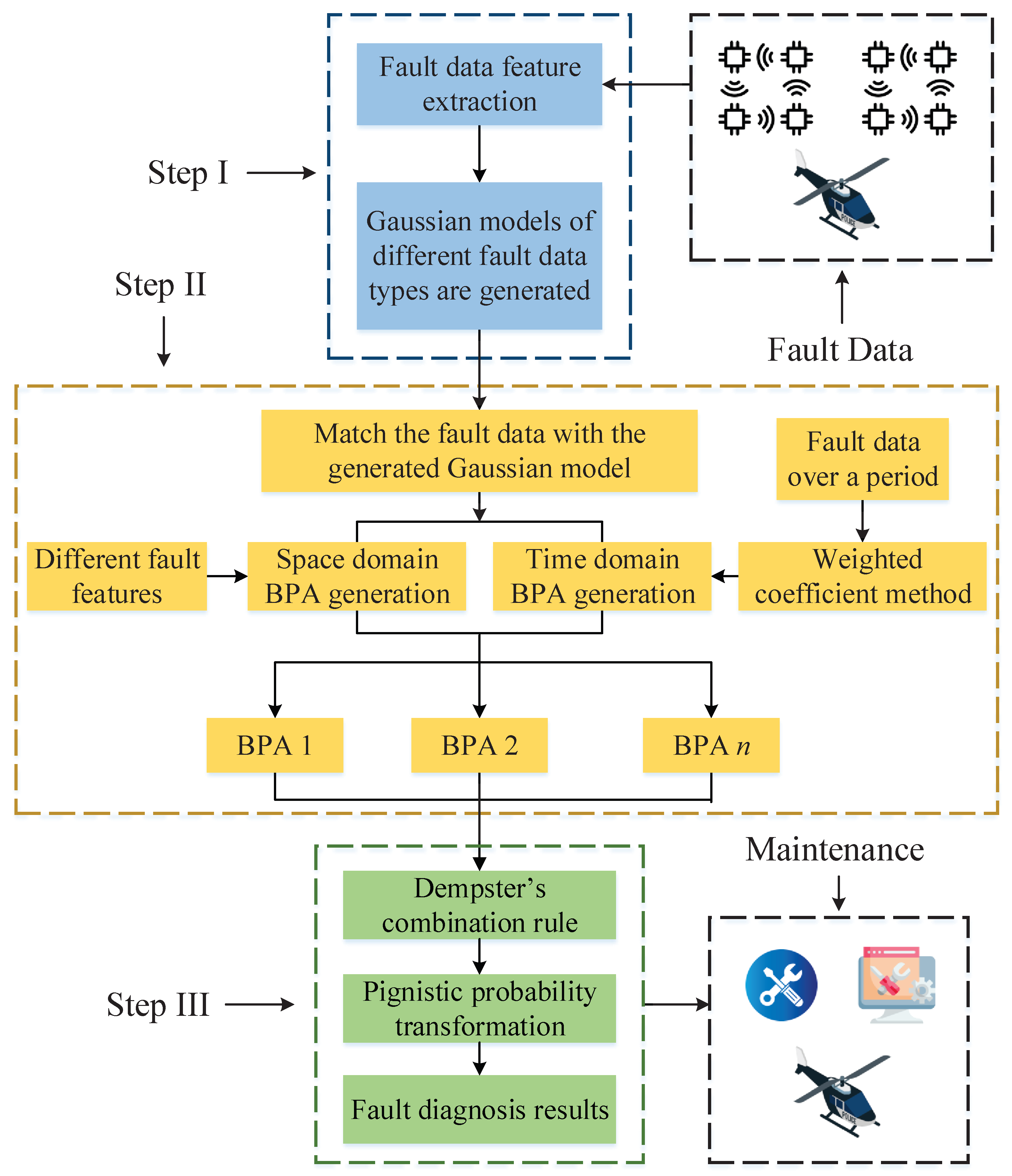
Figure 1 details the overall process of the proposed fault diagnosis method, consisting of three steps. According to the following steps, we can obtain the fault diagnosis results.

Figure 1.
The overall process of the proposed fault diagnosis method.
- Step I: Feature extraction of fault data is performed to construct the Gaussian fault model.
- Step II: In the time domain (multi-feature) and space domain (multi-moment), the fault data are fused to generate the BPAs. Additionally, in the time domain, the weighted coefficient method is used to fuse BPAs over a period.
- Step III: The BPAs generated in Part II are fused by using the Dempster’s combination rule. Then, the pignistic probability transformation is employed for decision-making.
2.1. Gaussian Fault Model
We define the Gaussian fault model with the fault type and fault feature as follows:
where X is the set whose fault type is and whose fault feature is . The steps for generating the Gaussian fault model of fault data with different features are as follows.
- Step I: We calculate the average value of the fault data with fault type and fault feature as follows:
- Step II: We calculate the standard deviation of the fault data with the fault type and fault feature as follows:
- Step III: Based on and , the constructed Gaussian fault model can be expressed as follows:
2.2. Time–Space Domain BPA Generation
In Section 2.2, we use the time–space domain combined information fusion method for fault diagnosis, where the BPAs are generated from both time and space domains.
2.2.1. Space Domain BPA Generation
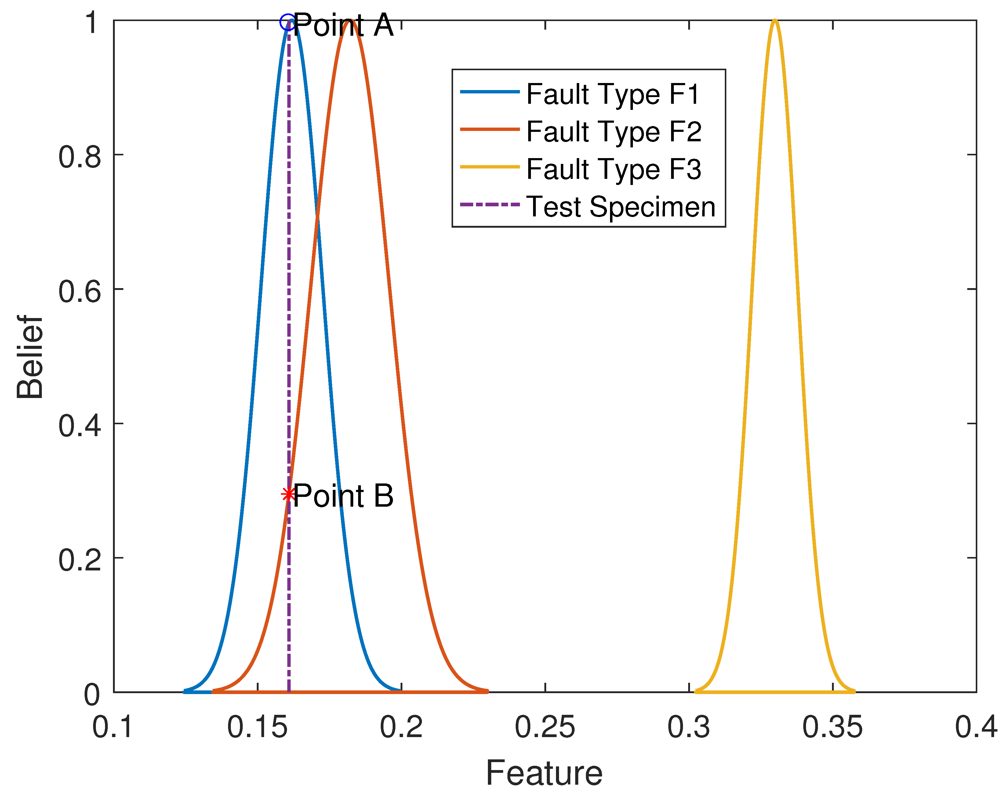
First, the generation of BPAs is implemented from the space domain (i.e., the feature of fault data). Specifically, according to (2) and (3), the average value and standard deviation of n different fault features are solved, respectively. Then, the Gaussian fault model with n different fault features is obtained. Based on the fault feature , we can obtain the constructed Gaussian fault model, as shown in Figure 2. We can find that the Gaussian model describes the central location and dispersion of data through their mean and variance parameters, providing a mathematical foundation for distinguishing between different fault types. Within the D-S evidence theory, each fault type’s Gaussian model not only reflects the typical characteristics of the fault but also expresses the uncertainty and similarity between different fault types through overlaps between models. Figure 2 is a simple example of a Gaussian fault model, including three types of faults. More precisely, the dashed line indicates the test specimen. The blue line, orange line, and yellow line indicate three different fault types, respectively. By constructing the Gaussian fault model, the similarity between test specimens and each fault model can be calculated. On this basis, we can determine the matching degree and BPA by the points of intersection between the test specimen and the constructed Gaussian fault model, i.e., points A and B.
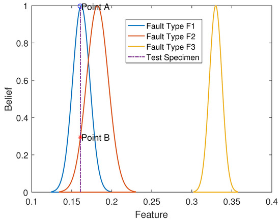
Figure 2.
A simple example of the Gaussian fault model: Since the fault features of UASs usually show an approximate normal (Gaussian) distribution, the Gaussian fault modes can be constructed for the proposed fault diagnosis methods.
2.2.2. Time-Domain BPA Generation
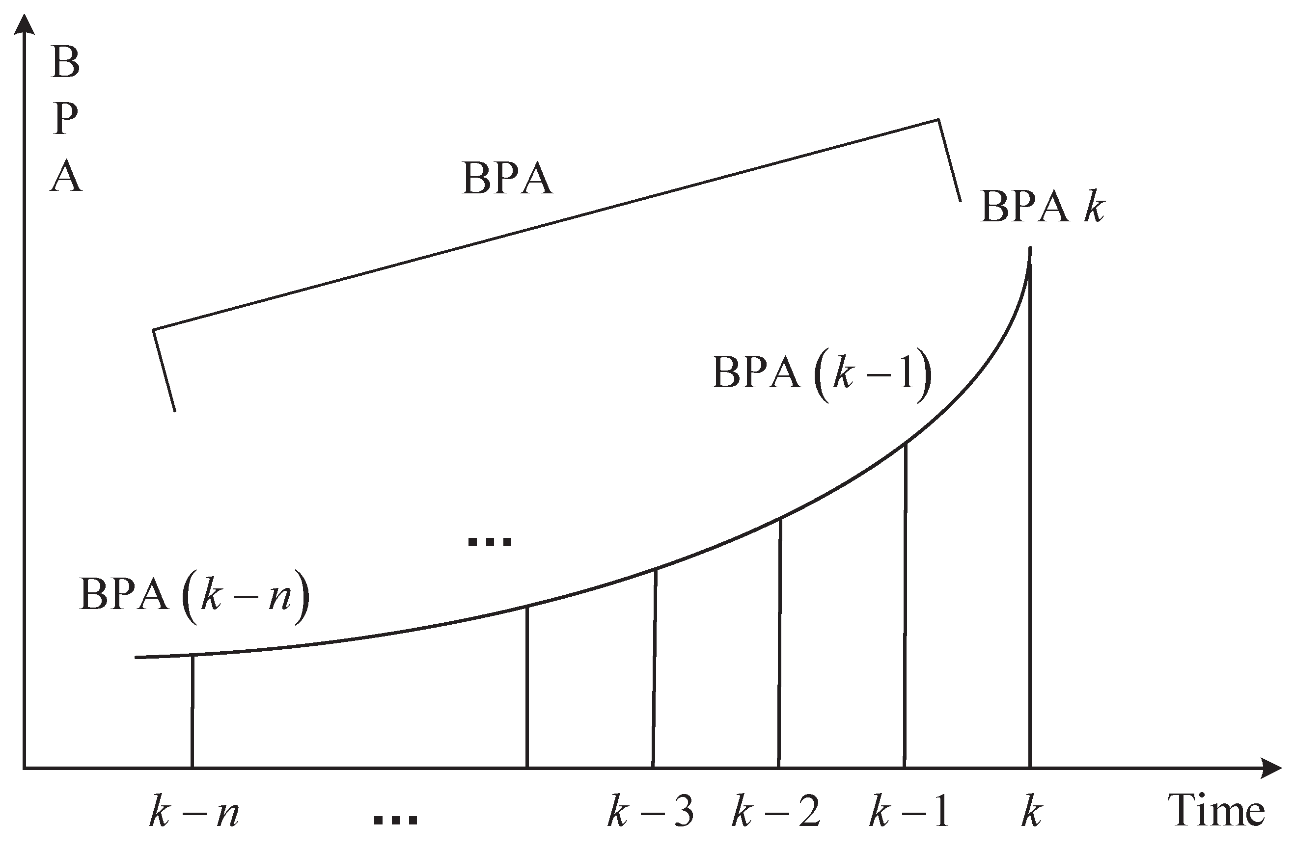
Because of the diversity and uncertainty of the fault data, it is not accurate to diagnose the fault solely from the feature. In this situation, time-domain information is considered. When the fault diagnosis is performed at time k, we select the fault data in at different times. The weighted coefficient method is used to deal with the weight of BPAs, i.e., BPAs in different times are generated from the test specimen. Then, these BPAs are weighted to obtain new BPAs. Figure 3 illustrates the generation of BPAs by using the weighted coefficient method. Specifically, the weighted coefficient method for processing BPAs refers to a technique used within the D-S evidence theory, which is aimed at combining evidence from various sources to manage uncertainty and incompleteness in information [36]. The key steps are as follows. First, a weight coefficient is assigned to each source based on its reliability, accuracy, or other relevant criteria. These weights are numeric values between 0 and 1, reflecting the trust level in the source. Second, each source’s BPA is adjusted according to its corresponding weight. For each possible proposition or set of propositions, its BPA value is multiplied by the respective weight to obtain the weighted BPA. Third, using Dempster’s combination rule, all the weighted BPAs are merged. The merging process accounts for potential conflicts among sources and adjusts the combined belief distribution accordingly. Finally, the merged BPA provides a comprehensive view of the truthfulness of different propositions, which can be used for decision support or further analysis.
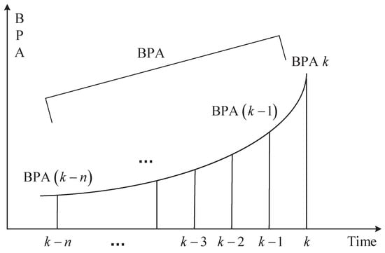
Figure 3.
A diagram of the generation of BPAs by using the weighted coefficient method: Each evidence source is assigned a weight based on its reliability. Then, the final BPA is calculated by adding these weighted values.
2.3. Information Fusion and Decision-Making
According to the D-S evidence theory, we use Dempster’s combination rule to fuse the BPAs generated in Section 2.1 [36,37,38]. Specifically, Dempster’s composition rule is a fundamental component of D-S evidence theory and is employed to systematically combine multiple belief functions into a single belief function. The Dempster’s combination rule operates by aggregating the BPAs from different sources, focusing on the intersection of evidence to compute the degree of belief for each proposition. Through normalization, it can ensure that the resultant belief function is a coherent representation of the combined evidence, which helps in making decisions based on aggregated and validated data. By integrating various evidence, our objective is to achieve information that is both logical and dependable while minimizing the uncertainty associated with the acquired data. However, since the fused BPAs may contain uncertainties, it is not conducive to making decisions. Thus, the BPAs can be converted to probabilities using the pignistic probability transformation, based on which the fault type of test specimens can be diagnosed. The pignistic probability transformation is defined as follows:
It is assumed that m is a BPA in FOD, and its pignistic probability transformation can be expressed as follows:
where is the power set of , and is the cardinal number of set Y.
Discussion: The integration of the time–space domain weighted information fusion and D-S evidence theory provides significant advantages for fault diagnosis in UASs by leveraging comprehensive data analysis and enhanced decision-making capabilities. By combining data across different times and locations, time–space fusion constructs a holistic view of the system’s operational status, facilitating the detection of abnormal patterns and potential faults more accurately. This approach is particularly effective in environments where sensor data may be uncertain or incomplete, as the D-S evidence theory excels in managing such uncertainties. It aggregates multiple sources of evidence to calculate probabilities of potential faults, providing a reliable basis for diagnostic assessments.
Moreover, the D-S theory enhances decision-making by quantifying the confidence levels associated with different diagnostic scenarios, allowing for prioritized and informed response strategies. This capability is critical in UASs where timely and accurate fault resolution is paramount. The fusion of time–space data and D-S theory support dynamic updating, enabling real-time system monitoring and immediate response to emerging faults. The adaptability of this methodology means that it can be applied across various time–space and operational scales, making it a versatile and robust tool for maintaining system reliability and performance.
3. Performance Evaluation
3.1. Simulation Environment
This section illustrates the application of the proposed fault diagnosis method by demonstrating its effectiveness in diagnosing motor rotor faults of UASs, as depicted in Figure 4. Specifically, on the left part of Figure 4, an operational schematic of the UAS in flight demonstrates its control and navigation mechanisms. On the right part of Figure 4, an expanded view of the motor rotors is highlighted for fault diagnosis, utilizing the proposed method to identify and analyze potential fault types within the rotors of UASs.
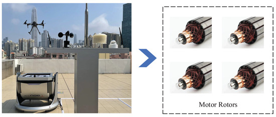
Figure 4.
A diagram of the considered UAS and the corresponding motor rotor for fault diagnosis.
In the simulation, fault data are collected from vibration signals using displacement and accelerometer sensors mounted on the rotor, from which key features are extracted. The simulation setup includes three common types of rotor faults (rotor imbalance, misalignment, and looseness of the base), denoted as . Normally, when the rotor faults, the vibration amplitude at any frequency does not exceed 0.1 m per second. If a fault occurs, the vibration amplitude will significantly increase, and different types of faults will cause changes in different vibration frequencies or bands.
To accurately diagnose the fault type, the simulation environment not only analyzes the vibration amplitude at each frequency but also specifically focuses on the vibration energy concentrated at 1× (fundamental frequency), 2× (second harmonic), and 3× (third harmonic). By combining the vibration amplitudes from 1× to 3× and the average amplitude of time-domain vibration displacement, a fault feature vector is formed to identify specific fault types. The fault features are defined as . Specifically, are the amplitudes of these three frequencies, and is the time-domain vibration displacement.
3.2. Numerical Results
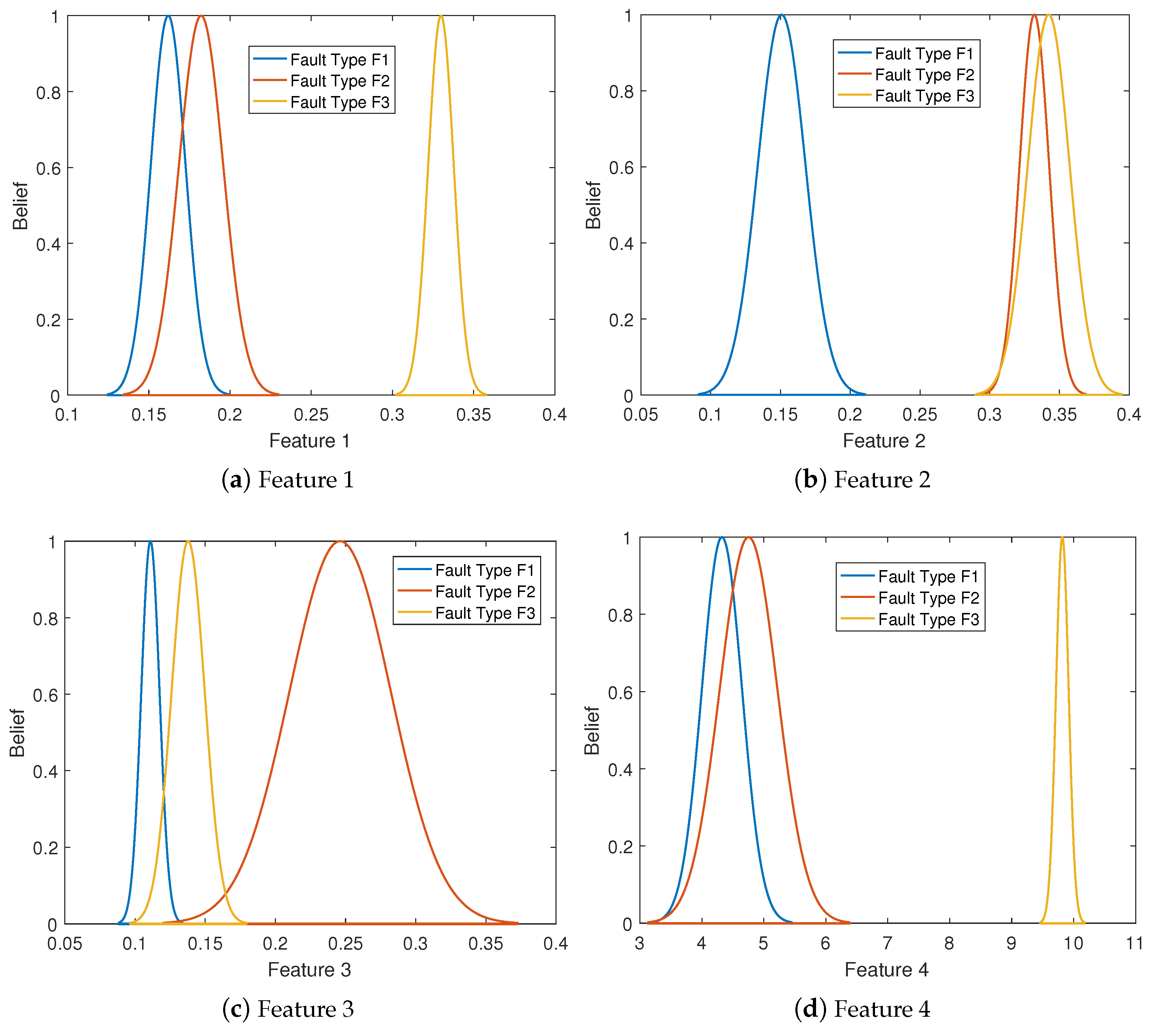
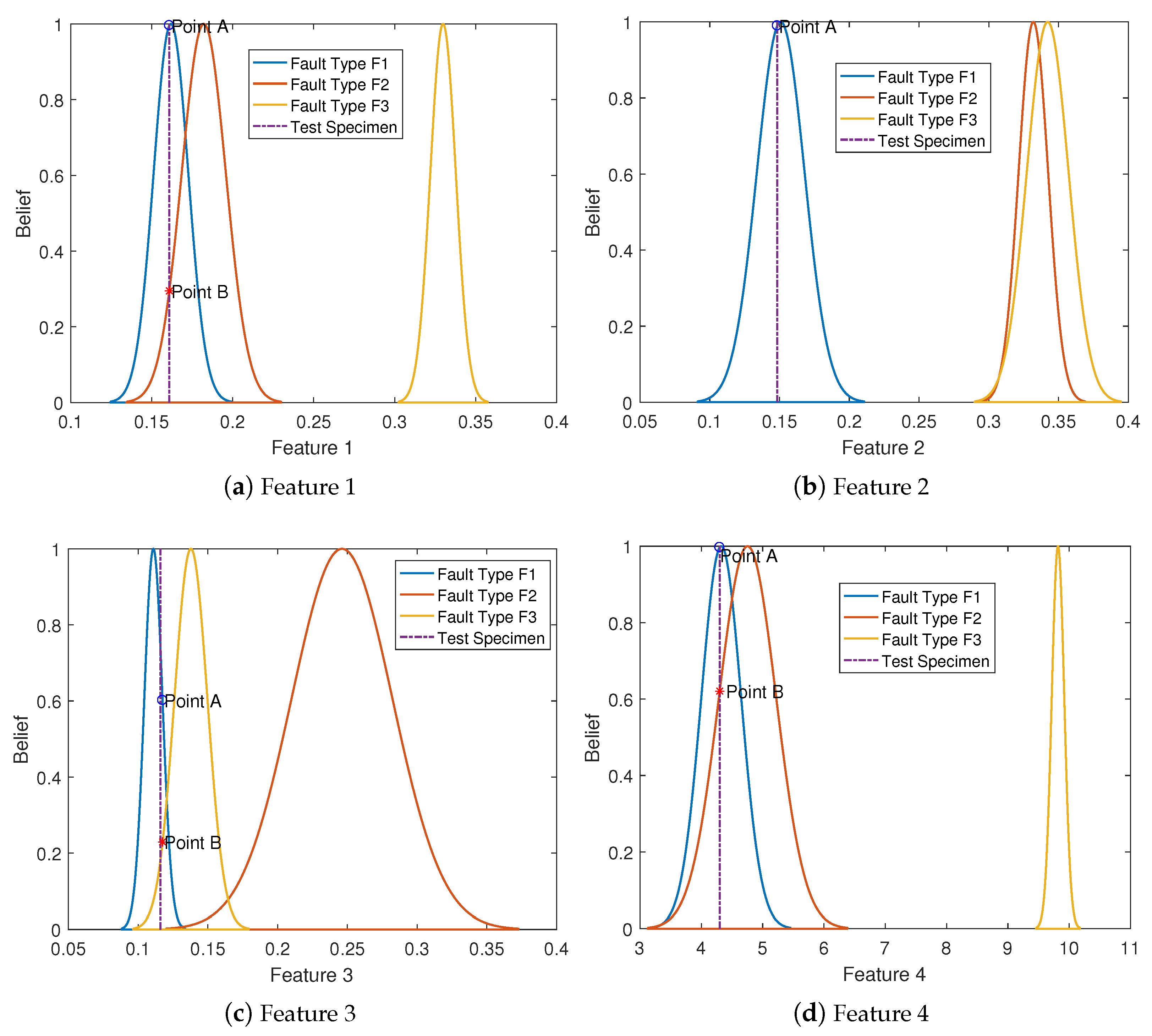
First, we calculate and by using (2) and (3). Based on (4), we can construct the Gaussian fault model, as shown in Figure 5a,b. Then, the fault data are matched with the generated Gaussian fault model as shown in Figure 6a,b. Based on this, Table 1 shows the time-domain BPAs under different fault features. As shown in Figure 6a,b, in the application of the proposed method for fault diagnosis, matching fault data with the generated Gaussian fault model aims to enhance the accuracy and reliability of fault diagnosis. The Gaussian model represents the statistical characteristics of faults. Matching the fault data with these models allows for more precise identification of faults within UASs, thereby pinpointing the fault types. Furthermore, as observed from Figure 6a,b, the generated Gaussian fault model effectively reduces the intersection areas between different fault features. This reduction in intersection areas indicates an improvement in the ability to identify fault features.
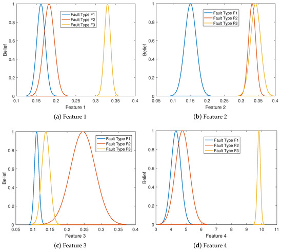
Figure 5.
A diagram of the constructed Gaussian fault model under different fault features: In a constructed Gaussian fault model based on different fault features, each feature is statistically analyzed to determine its mean and variance.
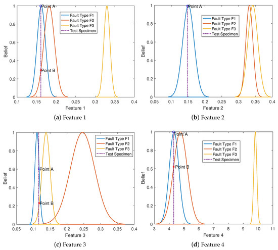
Figure 6.
The generation of BPAs in the space domain: Fault features are processed through Gaussian models to generate BPAs that diagnose the fault type.

Table 1.
The time-domain BPAs.
As previously discussed, we select the fault data in at different times. In our numerical simulations, , thereby generating 10 BPAs. By using the weighted coefficient method, we can obtain the time–space domain BPAs, as shown in Table 2. As shown in Table 2, the fault features provide specific information about the UASs, while fault types are inferred causes behind these features. In the proposed fault diagnosis method, we associate collected features with the probabilities of different fault types, thereby offering a quantitative approach to assess the likelihood of each fault type. Specifically, the fault features can be seen as sources of evidence used to update the belief and plausibility of various fault types. By combining and computing the beliefs associated with different features, we can infer the relative confidence in various fault types. Therefore, the fault features directly influence the estimation of probabilities for fault types.

Table 2.
The time–space domain BPAs.
Finally, using the Dempster’s combination rule fuses the time–space domain BPAs, and we have by performing normalization. Based on this, the pignistic probability transformation is employed, and we can obtain . According to the above results, we can find that the fault type is . The diagnosis result is consistent with the real fault type, which confirms the effectiveness of the proposed fault diagnosis method.
4. Conclusions
In this paper, we studied the fault diagnosis problem for UASs and presented a fault diagnosis method based on time–space domain weighted information fusion. Compared to the conventional fault diagnosis method based on time or space domain, the proposed fault diagnosis method had higher diagnostic accuracy and reliability. First, according to different fault features in the space domain, the Gaussian fault model was constructed, and the test specimens were matched with the constructed Gaussian fault model to obtain the corresponding BPAs. Since the uncertainty of fault diagnosis at a single moment was high, the Gaussian fault model was constructed by using different fault features over a period. Then, the weighted coefficient method was adopted to obtain the time–space domain BPAs. Afterward, the Dempster’s combination rule was employed to fuse the generated BPAs, where the normalization was performed. Finally, by using the pignistic probability transformation, we obtained the fault type. Through numerical simulations, we verified the efficacy of the proposed fault diagnosis method.
However, the proposed fault diagnosis method has its shortcomings. On the one hand, the fault features are self-defined, which might not comprehensively represent actual operational scenarios. This limitation could possibly restrict the method’s accuracy and general applicability across different UAS operations. On the other hand, the paper lacks a thorough analysis of the UAS’s reliability under varied and real-world conditions, focusing only on idealized fault scenarios. Addressing these gaps, especially through leveraging insights from [39,40], could enhance the development of more robust and reliable fault diagnosis solutions for UASs or drone fleets.
For future work on the fault diagnosis of UASs, several key areas can be explored and improved.
- Real-time fault diagnosis: In UASs, real-time fault diagnosis is essential for preventing system failures and reducing downtime. Future research can concentrate on developing efficient and low-latency fusion algorithms that can provide timely fault diagnosis and enable proactive maintenance.
- Multi-modal information fusion: Instead of only considering time and space domains, integrating data from various modalities, such as frequency domain or image data, can further improve the accuracy and robustness of fault diagnosis. Combining data from different sources can offer complementary information and lead to a more comprehensive understanding of the system’s health.
- Uncertainty quantification: Fault diagnosis methods of UASs should be capable of estimating and quantifying uncertainties in their predictions. This is crucial in high-stakes applications where the reliability of diagnosis plays a vital role. Uncertainty estimation can provide confidence intervals for fault predictions and enhance decision-making processes.
Author Contributions
N.L.: formal analysis, investigation, methodology, software, validation, visualization, and writing—review and editing. Z.Z.: conceptualization, methodology, software, and writing—original draft preparation. L.Z.: data curation, resources, and funding acquisition. Y.H.: conceptualization, resources, writing—review and editing, supervision, and funding acquisition. F.H.: conceptualization, methodology, and formal analysis. All authors have read and agreed to the published version of the manuscript.
Funding
This work was supported in part by the “Pioneer” and “Leading Goose” R&D Program of Zhejiang under grant nos. 2024C04004 and 2023C01162, in part by the Zhejiang Provincial Natural Science Foundation of China under grant LQ24F010003, in part by the University-Industry Collaborative Education Program under Grant 231000287070509, and in part by the China National University Student Innovation & Entrepreneurship Development Program under Grant 202410354039.
Data Availability Statement
Data are contained within the article.
Conflicts of Interest
The authors declare no conflicts of interest.
References
- Schweiger, K.; Preis, L. Urban air mobility: Systematic review of scientific publications and regulations for vertiport design and operation. Drones 2022, 6, 179. [Google Scholar] [CrossRef]
- He, Y.; Wang, D.; Huang, F.; Zhang, R.; Min, L. Aerial-ground integrated vehicular networks: A UAV-vehicle collaboration perspective. IEEE Trans. Intell. Transp. Syst. 2024, 25, 5154–5169. [Google Scholar] [CrossRef]
- Dai, M.; Luan, T.H.; Su, Z.; Zhang, N.; Xu, Q.; Li, R. Joint channel allocation and data delivery for UAV-assisted cooperative transportation communications in post-disaster networks. IEEE Trans. Intell. Transp. Syst. 2022, 23, 16676–16689. [Google Scholar] [CrossRef]
- He, Y.; Wang, D.; Huang, F.; Zhang, R.; Gu, X.; Pan, J. A V2I and V2V collaboration framework to support emergency communications in ABS-aided Internet of Vehicles. IEEE Trans. Green Commun. Netw. 2023, 7, 2038–2051. [Google Scholar] [CrossRef]
- Yuan, Q.; Lv, M.; Zhou, R.; Liu, H.; Liang, C.; Cheng, L. Use of composite multivariate multiscale permutation fuzzy entropy to diagnose the faults of rolling bearing. Entropy 2023, 25, 1049. [Google Scholar] [CrossRef] [PubMed]
- Gao, Z.; Cecati, C.; Ding, S.X. A survey of fault diagnosis and fault-tolerant techniques–Part II: Fault diagnosis with knowledge-based and hybrid/active approaches. IEEE Trans. Ind. Electron. 2015, 62, 3768–3774. [Google Scholar] [CrossRef]
- Hu, Q.; Qin, A.; Zhang, Q.; He, J.; Sun, G. Fault diagnosis based on weighted extreme learning machine with wavelet packet decomposition and KPCA. IEEE Sens. J. 2018, 18, 8472–8483. [Google Scholar] [CrossRef]
- Ciaburro, G. Machine fault detection methods based on machine learning algorithms: A review. Math. Biosci. Eng. 2019, 19, 11453–11490. [Google Scholar] [CrossRef] [PubMed]
- Shraim, H.; Awada, A.; Youness, R. A survey on quadrotors: Configurations, modeling and identification, control, collision avoidance, fault diagnosis and tolerant control. IEEE Aerosp. Electron. Syst. Mag. 2018, 33, 14–33. [Google Scholar] [CrossRef]
- Peng, B.; Bi, Y.; Xue, B.; Zhang, M.; Wan, S. Multi-view feature construction using genetic programming for rolling bearing fault diagnosis [application notes]. IEEE Comput. Intell. Mag. 2021, 16, 79–94. [Google Scholar] [CrossRef]
- Zhang, X.; Luo, H.; Li, K.; Kaynak, O. Time-domain frequency estimation with application to fault diagnosis of the unmanned aerial vehicles’ blade damage. IEEE Trans. Ind. Electron. 2022, 69, 5257–5266. [Google Scholar] [CrossRef]
- Rudin, K.; Ducard, G.J.J.; Siegwart, R.Y. Active fault-tolerant control with imperfect fault detection information: Applications to UAVs. IEEE Trans. Aerosp. Electron. Syst. 2020, 56, 2792–2805. [Google Scholar] [CrossRef]
- Wang, B.; Peng, X.; Jiang, M.; Liu, D. Real-time fault detection for UAV based on model acceleration engine. IEEE Trans. Instrum. Meas. 2020, 69, 9505–9516. [Google Scholar] [CrossRef]
- Cao, Y.; Yang, J.-B.; Deng, X.; Jiang, W. The fusion of discrete Z-numbers with application for fault diagnosis. IEEE Trans. Instrum. Meas. 2022, 71, 2516615. [Google Scholar] [CrossRef]
- Zhang, Z.; Jiang, W.; Geng, J.; Deng, X.; Li, X. Fault diagnosis based on non-negative sparse constrained deep neural networks and Dempster-Shafer theory. IEEE Access 2020, 8, 18182–18195. [Google Scholar] [CrossRef]
- Ramu, S.K.; Vairavasundaram, I.; Aljafari, B.; Kareri, T. Rotor bar fault diagnosis in indirect field-oriented control-fed induction motor drive using hilbert transform, discrete wavelet transform, and energy eigenvalue computation. Machines 2023, 11, 711. [Google Scholar] [CrossRef]
- Ahmed, H.O.A.; Nandi, A.K. Convolutional-transformer model with long-range temporal dependencies for bearing fault diagnosis using vibration signals. Machines 2023, 11, 746. [Google Scholar] [CrossRef]
- Li, M.; Zhou, Y.; Jia, L.; Qin, Y.; Wang, Z. Sequential-fault diagnosis strategy for high-speed train traction systems based on unreliable tests. Appl. Sci. 2023, 13, 8226. [Google Scholar] [CrossRef]
- Huang, F.; He, Y.; Deng, X.; Jiang, W. A novel discount-weighted average fusion method based on reinforcement learning for conflicting data. IEEE Syst. J. 2023, 17, 4748–4751. [Google Scholar] [CrossRef]
- Kim, H.; Lee, H.; Kim, S.; Kim, S.W. Attention recurrent neural network-based severity estimation method for early-stage fault diagnosis in robot harness cable. Sensors 2023, 23, 5299. [Google Scholar] [CrossRef]
- Ciaburro, G.; Padmanabhan, S.; Maleh, Y.; Puyana-Romero, V. Fan Fault Diagnosis Using Acoustic Emission and Deep Learning Methods. Informatics 2023, 10, 24. [Google Scholar] [CrossRef]
- Iannace, G.; Ciaburro, G.; Trematerra, A. Fault diagnosis for UAV blades using artificial neural network. Robotics 2019, 8, 59. [Google Scholar] [CrossRef]
- Wan, S.; Li, T.; Fang, B.; Yan, K.; Hong, J.; Li, X. Bearing fault diagnosis based on multisensor information coupling and attentional feature fusion. IEEE Trans. Instrum. Meas. 2023, 72, 3514412. [Google Scholar] [CrossRef]
- Xiong, J.; Zhang, Q.; Sun, G.; Zhu, X.; Liu, M.; Li, Z. An information fusion fault diagnosis method based on dimensionless indicators with static discounting factor and KNN. IEEE Sens. J. 2016, 16, 2060–2069. [Google Scholar] [CrossRef]
- Hoang, D.T.; Kang, H.J. A motor current signal-based bearing fault diagnosis using deep learning and information fusion. IEEE Trans. Instrum. Meas. 2020, 69, 3325–3333. [Google Scholar] [CrossRef]
- Gao, X.; Pan, L.; Deng, Y. Quantum pythagorean fuzzy evidence theory: A negation of quantum mass function view. IEEE Trans. Fuzzy Syst. 2022, 30, 1313–1327. [Google Scholar] [CrossRef]
- Zhao, J.; Deng, Y. Complex network modeling of evidence theory. IEEE Trans. Fuzzy Syst. 2021, 29, 3470–3480. [Google Scholar] [CrossRef]
- Liu, Q. Coverage reliability evaluation of wireless sensor network considering common cause failures based on D-S evidence theory. IEEE Trans. Reliab. 2021, 70, 331–345. [Google Scholar] [CrossRef]
- Wang, F.; Liu, Y.; Wang, Y.; Wu, K.; Wu, D. A Multisensor Approach Integrating Cyclostationary Analysis and Evidence Theory for Explainable Bearing Fault Diagnosis. IEEE Sens. J. 2024, 24, 17885–17895. [Google Scholar] [CrossRef]
- Ding, W.; Sun, Y.; Li, M.; Liu, J.; Ju, H.; Huang, J.; Lin, C.T. A Novel Spark-Based Attribute Reduction and Neighborhood Classification for Rough Evidence. IEEE Trans. Cybern. 2024, 54, 1470–1483. [Google Scholar] [CrossRef]
- Ma, Y.; Zhang, J.; Qin, G.; Jin, J.; Zhang, K.; Pan, D.; Chen, M. 3D Multi-Object Tracking Based on Dual-Tracker and D-S Evidence Theory. IEEE Trans. Intell. Veh. 2023, 8, 2426–2436. [Google Scholar] [CrossRef]
- Wang, H.; Lin, D.; Qiu, J.; Ao, L.; Du, Z.; He, B. Research on multiobjective group decision-making in condition-based maintenance for transmission and transformation equipment based on D-S evidence theory. IEEE Trans. Smart Grid 2015, 6, 1035–1045. [Google Scholar] [CrossRef]
- Liu, Y.; Li, Z.; Zhang, L.; Fu, H. Fault Diagnosis Method for Space Fluid Loop Systems Based on Improved Evidence Theory. Entropy 2024, 26, 427. [Google Scholar] [CrossRef] [PubMed]
- Jiang, D.; Wang, Z. Research on Mechanical Equipment Fault Diagnosis Method Based on Deep Learning and Information Fusion. Sensors 2023, 23, 6999. [Google Scholar] [CrossRef] [PubMed]
- Liang, X.; Luo, Y.; Deng, F.; Li, Y. Application of Improved MFDFA and D-S Evidence Theory in Fault Diagnosis. Appl. Sci. 2022, 12, 4976. [Google Scholar] [CrossRef]
- Zhang, Y.; Jiang, W.; Deng, X. Fault diagnosis method based on time domain weighted data aggregation and information fusion. Int. Distrib. J. Sens. Netw. 2019, 15. [Google Scholar] [CrossRef]
- Zhang, W.; Sun, H.; Fang, W.; Zhu, C.; Jia, G. Trust Evaluation and Decision Based on D-S Evidence Theory: Early Models and Future Perspectives. IEEE Access 2023, 11, 16032–16041. [Google Scholar] [CrossRef]
- Tang, Y.; Wu, S.; Zhou, Y.; Huang, Y.; Zhou, D. A New Reliability Coefficient Using Betting Commitment Evidence Distance in Dempster–Shafer Evidence Theory for Uncertain Information Fusion. Entropy 2023, 25, 462. [Google Scholar] [CrossRef] [PubMed]
- Zaitseva, E.; Levashenko, V.; Mukhamediev, R.; Brinzei, N.; Kovalenko, A.; Symagulov, A. Review of Reliability Assessment Methods of Drone Swarm (Fleet) and a New Importance Evaluation Based Method of Drone Swarm Structure Analysis. Mathematics 2023, 11, 2551. [Google Scholar] [CrossRef]
- Marek, D.; Paszkuta, M.; Szyguła, J.; Biernacki, P.; Domański, A.; Szczygieł, M.; Król, M.; Wojciechowski, K. Swarm of Drones in a Simulation Environment—Efficiency and Adaptation. Appl. Sci. 2024, 14, 3703. [Google Scholar] [CrossRef]
Disclaimer/Publisher’s Note: The statements, opinions and data contained in all publications are solely those of the individual author(s) and contributor(s) and not of MDPI and/or the editor(s). MDPI and/or the editor(s) disclaim responsibility for any injury to people or property resulting from any ideas, methods, instructions or products referred to in the content. |
© 2024 by the authors. Licensee MDPI, Basel, Switzerland. This article is an open access article distributed under the terms and conditions of the Creative Commons Attribution (CC BY) license (https://creativecommons.org/licenses/by/4.0/).

