Abstract
The nonlinear characteristics of the pneumatic servo system are the main factors limiting its control accuracy. A new mathematical model of the nonlinear system of the valve control cylinder is proposed in order to improve the control accuracy of the pneumatic servo system. Firstly, the mass flow equation of the gas flowing through each port is established by analyzing the physical structure of the proportional directional control valve. Then, the dynamic equation of the system is set up by applying the Stribeck friction model for the friction model of the valve control cylinder and building a pneumatic circuit experiment to identify the friction model parameters. Finally, the correctness of the mathematical model is verified by the inflation and deflation experiment of the fixed capacitive chamber and the servo controls experiment based on PID position. The Simulink simulation of the mathematical model better reflects the characteristics of the pneumatic position servo system.
1. Introduction
Pneumatic technology, also known as pneumatic transmission technology, is a technology that uses an air compressor as the power source to realize the automatic production of various industries. It can also be said that it is an effective means to use compressed gas as a working medium to realize the transmission of energy and signals and achieve the purpose of mechanization and automation of the production process [1]. After a long period of development, pneumatic technology has now become one of the three major drive technologies in the machinery industry and has been applied in various industries [2,3,4]. Compared with mechanical transmission, electric transmission and hydraulic transmission, pneumatic technology has the characteristics of zero pollution, safety and reliability, simple structure and low cost. Under the advocacy of the modern green development concept, pneumatic technology has good development prospects [5].
Because the pneumatic servo drive has the advantages of compact structure, small volume, convenient installation and fewer control parameters, scholars at home and abroad gradually began to increase their research on it. The magnetically coupled rodless cylinder is widely used in the positioning of mechanical arm coordinates, electrostatic painting and other industrial occasions [6]. However, through a survey, it was found that most of the commodities exported to foreign countries in China are low-end products, and there are relatively few products with higher technical requirements. Most of the reasons are due to the relatively high accuracy requirements of high-end position servo control accuracy requirements products. The main reasons affecting pneumatic servo position control accuracy are: (1) there are often many unknown parameters in the pneumatic servo system model, and these parameters have a great impact on the position control effect of the servo system. Therefore, these unknown parameters also need to be identified. (2) The pneumatic system itself has strong nonlinear characteristics and model uncertainty. In order to solve the position control problem of the pneumatic system, most scholars generally use the method of linearizing the mathematical model of a nonlinear dynamic system near the ideal working position. However, if the model state of motion deviates too far from the ideal operating point, all analysis and design lose practical significance [7,8]. Therefore, based on the nonlinear characteristics of the pneumatic servo system [9,10], a more accurate nonlinear mathematical model needs to be established.
The nonlinearity of the pneumatic servo system is mainly manifested in the nonlinearity of the system model, the nonlinearity of the proportional valve flow equation and the nonlinearity of the friction force in the actuator. The nonlinearity of the pneumatic servo system is not only the main reason affecting the control accuracy of the servo system; it also brings great difficulties to the mathematical modeling of the servo system. Early on, Hearer and Blackburn [11] studied servo systems, and they built mathematical models of the pneumatic servo system using the transfer function method, but such mathematical models had limitations and only applied to the pistons in the cylinders working at the midpoint. Scavanda [12] extended the mathematical model of the linearized pneumatic servo system to multiple operating positions by applying the state-space method while ignoring nonlinear factors such as the friction of the cylinder during motion. The fifth-order nonlinear mathematical model proposed by Valdiero and Antonio et al. [13] expresses the main features of this nonlinear dynamic system, such as the servo valve dead zone, the airflow–pressure relationship through the valve bore, the air compressibility and the friction effect between the actuator seal and the contact surface. The simulation results show the dynamic performance of the different cylinders, making it easy to understand the impact of certain characteristics on the performance of the system. Bai [14] of Taiyuan University of Science and Technology established a position servo system for an oscillating cylinder through the study of the nonlinear characteristics of the proportional valve, the nonlinear characteristics of friction and the limit of the actuator at the end. Finally, the correctness of the simulation model was verified by simulation and experiments.
In this paper, in order to accurately establish the mathematical model of the nonlinear position servo system of the magnetically coupled rodless cylinder and consider the influence of the gap between the valve core and the sleeve, the mass flow rate of each valve gas body flowing through the proportional directional control valve is obtained. The friction model of the system is established by applying the Stribeck friction model to the friction model of the valve control cylinder, and a pneumatic circuit experiment is built to identify the friction model parameters. Finally, the dynamic equation of the system is established. The correctness of the mathematical model of the nonlinear system of the valve control cylinder is verified by the filling and venting experiment of the fixed capacity chamber and the position servo control experiment based on PID.
2. Experimental Set-Up
Figure 1 represents the experimental principle of the magnetically coupled rodless cylinder position servo system. The solid line represents the pneumatic connection, and the dashed line indicates the circuit connection. The compressed air produced by the compressor can be filtered, decompressed and dried through the pneumatic triplet (air filter, regulator and lubricator), providing a stable pressure to the system. The system selects a three-position five-way proportional directional control valve as the pneumatic control element of the system by use of a tie-rod displacement sensor to measure the displacement of the magnetically coupled rodless cylinder and a pressure transmitter to measure the supply pressure and the pressure of the two chambers of the cylinder. The tie-rod displacement sensor and pressure transmitter can produce a 1–5 V analog voltage signal. The data acquisition card is collected after the data acquisition. It can also convert the digital signal into an analog voltage signal. Through the collection and processing of the signal, the flow and flow direction of the gas at the two valve ports can be changed to accurately control the movement of the magnetically coupled rodless cylinder.
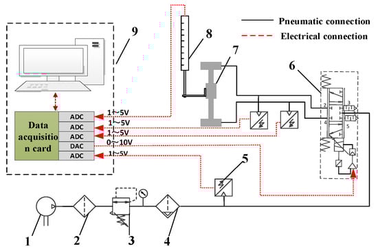
Figure 1.
Schematic of the servo control system for the position of the magnetically even rodless cylinder (1—air compressor; 2—air filter; 3—air regulator; 4—air lubricator; 5—pressure transmitter; 6—proportional directional control valve; 7—magnetically coupled rodless cylinder; 8— pull-rod displacement sensor; 9—IPC).
Figure 2 shows the experimental platform for the magnetically coupled rodless cylinder position servo system. The magnetically coupled rodless cylinder is fixed on a horizontal guide rail, and the proportional directional control valve is parallel to the horizontal plane. The models of the main components are shown in Table 1.
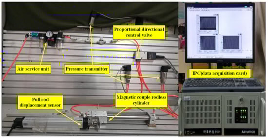
Figure 2.
Experimental platform of the magnetic even rodless cylinder position servo control system.

Table 1.
Main components of the system.
3. Establishment of the Mass Flow Equation for Proportional Directional Control Valves
The gas flow principle of the valve control cylinder system is shown in Figure 3. Ports 2 and 4 of the proportional directional control valve are connected to the two ends of the magnetically coupled rodless cylinder, assuming that the left and right chambers of the cylinder are Chambers A and B. The left-and-right movement of the spool of the proportional directional control valve changes the flow direction of the gas and realizes the left-and-right round-trip movement of the piston in the cylinder. , in the figure show the mass flow of the control valve flowing through the proportional direction to the two chamber gases of the cylinder. , represent the pressure of the two chambers of the cylinder. , show the volume of the two chambers of the cylinder. , indicate the temperature of the two chambers in the cylinder. m represents the mass of the load, and indicates the displacement of the piston in the cylinder. In addition, , indicate atmospheric pressure and supply pressure, respectively.
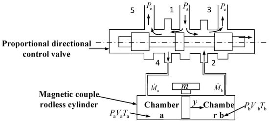
Figure 3.
Gas flow schematic for valve control cylinder systems.
Due to the complex flow characteristics of gases such as viscosity and compressibility, in order to simplify the mathematical model of valve control cylinder systems, the following assumptions are made [15,16]:
- (1)
- The air used in the system is an ideal gas;
- (2)
- When the gas flows through the proportional directional control valve and cylinder, it is regarded as an isentropic insulation state;
- (3)
- The gas pressure and temperature in the same chamber are equal everywhere;
- (4)
- During the left-and-right round-trip movement of the piston in the cylinder, the heat exchange between the gas inside the two chambers and the outside world does not occur as an insulation process;
- (5)
- The pressure and temperature of the gas supply are not affected by the external surrounding environment and remain constant.
3.1. Establishment of Mass Flow Equation When the Spool Is Moving Forward
Assuming that the spool of the proportional directional control valve is moved to the right, it is a positive movement. As shown in Figure 4, due to the movement of the valve spool to the right, the left side of Port 1 becomes a throttle hole, the right side becomes a gap and Ports 5 and 3 become a gap and a throttle, respectively. After the gas flows in from Port 1, most of it will flow into the chamber through the left side of Port 1. On the other hand, a small part of the gas flowing into the chamber on the left side of Port 1 will enter the atmosphere through the gap out of Port 5. On the left side of Port 1, it will flow into Chamber A of the cylinder through Port 4. The mass flow of gas flowing through Port 4 at this time is equal to the mass flow of gas flowing into Chamber A of the cylinder. Therefore, the difference between the mass flow of the gas flowing into Port 1 of the valve and the mass flow of gas flowing to the atmosphere from Port 5 of the valve is the mass flow of Chamber A of the cylinder.
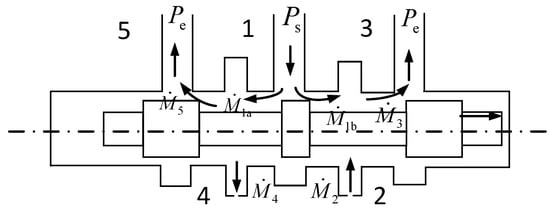
Figure 4.
Proportional directional control valve core forward movement of the flow schematic of the gas.
Since Port 2 of the proportional directional control valve is connected to Chamber B of the cylinder, the mass flow of gas flowing into the valve body through Port 2 is equal to the mass flow of Chamber b. The difference between the mass flow of gas flowing in from the right side of Port 1 and the mass flow is the mass flow of Chamber B of the cylinder.
3.2. Establishment of the Mass Flow Equation for Gases at the Orifice
When the spool of the proportional directional control valve is moved to the right, two throttle holes are formed in the same vertical direction of the valve body. After passing through these two throttles, the gas enters the chamber or atmosphere of the cylinder, respectively. There is a slight gap between the sleeve and the spool, as shown in Figure 5, so the mass flow of the gas in the horizontal direction and the mass flow in the vertical direction are the mass flow ,
where represents the gap between the spool and the sleeve; indicates the inner diameter of the sleeve, with a value of 0.006023 m; represents the outer diameter between the spool tables, with a value of 0.006 m; and is:
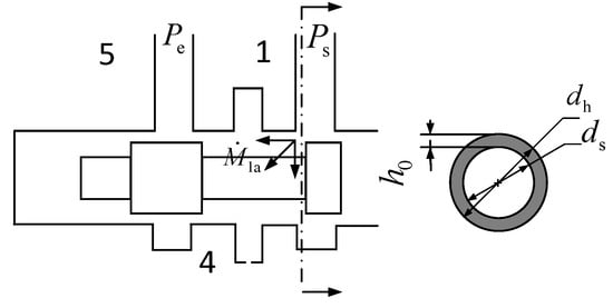
Figure 5.
Shunt flow of the throttle hole.
Due to the nonlinear relationship between the opening area of the proportional directional control valve port and the control voltage, it cannot be measured directly with an effective measuring tool. Bai [17] and Li [18] deduced the mathematical relationship between the valve spool displacement and the opening geometry of the proportional directional control valve by analyzing the position state of the spool during the movement. In this paper, the volume flow rate of the valve gas body is measured by building an experimental platform, the volume flow rate is brought into the volume flow formula in the standard state and, finally, the effective area of the valve opening is calculated.
Formula:
—Effective area of the valve opening, mm2;
—Absolute pressure upstream of the valve body, MPa;
—Temperature upstream of the valve body, K;
—Volume flow through the valve port, L/min.
The volume flow measurement method is shown in Figure 6: the supply pressure is set to 0.4 MPa and remains unchanged. The control voltage is adjusted from 0 V to 10 V and then from 10 V to 0 V, and the volume flow rate flowing through the proportional directional valve port under different control voltages is measured. The experiment is repeated three times. The results of the experiment are added to obtain the average, then substituted into Equation (4) to calculate the effective area of the valve opening. Finally, the numerical values of the control voltage and the effective area of the valve opening are brought into the fitting toolbox in MATLAB. The mathematical relationship between the effective area of the valve opening and the voltage change is obtained by using the polynomial fitting method. The results are shown in Figure 7.
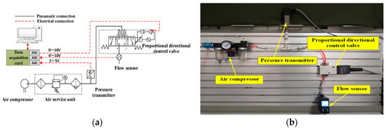
Figure 6.
Pneumatic circuit diagram: (a) schematic; (b) experimental test platform.
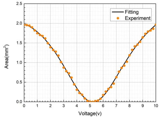
Figure 7.
Graph of the effective area and control voltage.
The mathematical relationship between the effective area of the valve opening and the control voltage is obtained by using the polynomial fitting method as follows:
According to Professor Sanville, the mass flow equation for gases flowing through the orifice is [19]:
where the gas constant is 8.31432 × 10³ J·mol−1·K−1, with a critical pressure ratio b of 0.528 and an equal entropy index k of 1.4, and Cv represents a flow coefficient.
3.3. Establishment of the Mass Flow Equation for Gases at Gaps
The flow state of the gas in the gap between the valve body of the proportional directional control valve is the same as the flow state between two panels parallel to each other. Figure 8 is a schematic diagram of the flow of the gas in the gap at Port 5 of the valve when the spool of the proportional directional control valve moves in the positive direction. With reference to the gap flow equation between the parallel plates [20], the differential equation of gas pressure can be derived:
where P is the gas microelement pressure in the gap; is the viscosity coefficient of the gas, with a value of 0.0000183; u is the speed of the gas microelement in the x-direction; indicates the initial length of the gap, with a value of 0.002 m; and indicates the displacement of the valve spool.
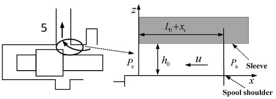
Figure 8.
Schematic of valve core clearance flow.
The constraints on its boundaries are:
and
Combining Equations (8) and (9) gives the gas velocity formula in the gap:
The mass flow rate of the gas flowing through the gap is:
where is the density of the gas.
Because the gap size of the parallel plate is fixed along the -direction, the pressure of the gas in the gap will gradually increase as the shaft increases. Combined with Equation (10), it yields:
According to the equation of state of the gas, it obtains:
Bringing Equations (3), (11), (13) and (14) into Equation (12) gives the mathematical expression of the mass flow of gas flowing through Port 5:
The mathematical expressions of available for the same reasoning are:
3.4. Establishment of the Mass Flow Equation When the Spool Moves in Reverse
As shown in Figure 9, during the reverse movement of the spool of the proportional control valve, most of the gas flows from the throttle hole on the right side of Port 1 of the valve into the capacity chamber on the right side of the valve body, and then part of the gas flows out of the gap at Port 3 of the valve. The gas flowing in from the gap on the left side of Port 1 of the valve enters the chamber on the left side of the valve body. Finally, it is discharged into the atmosphere through the throttle hole of Port 5 of the valve.
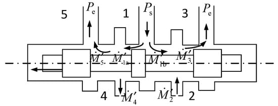
Figure 9.
Directional control valve core Is moving in gas flow schematic.
During the forward and reverse movement of the proportional directional control valve core, the spool of a proportional directional control valve has the same mathematical relationship:
The mass flow equation for gases through the throttle hole is:
The mass flow equation for the gap gas is:
3.5. Measurement of Flow Coefficient of Proportional Directional Valve
In the experimental test delivery pipeline, when the pressure of the gas remains constant, the gas flow rate coefficient can be expressed as the mass gas flow through the valve port (the valve port flow rate). The pressure loss when the gas flows through the valve port is inversely proportional to ; that is, the larger the flow coefficient, the greater the flow capacity of the gas to flow through the valve port. The value of the flow coefficient can only be determined under the conditions of experimental tests and formula calculations.
Test principle of the flow coefficient: With the change in the control voltage, the effective opening area of the valve port will also change. Since the flow capacity is related to the change of the flow coefficient, it is necessary to measure the mass flow of the valve port at different voltages and then calculate the different flow coefficients. The calculated value of the quantity coefficient can be brought into MATLAB’s fitting toolbox, and the mathematical relationship between the flow coefficient and the control voltage can be polynomially fitted [21]. According to Equations (1), (5) and (6), the value of the flow coefficient can be calculated by:
Experimental test of flow coefficient is shown in Figure 10: The supply pressure of the experimental test is 0.5 MPa, and the temperature is set to 297 k. Pressure sensors and flow sensors are used to measure the value of supply pressure and mass flow , at Ports 4 and 5. Finally, Formula (23) is brought in to calculate the value of the flow coefficient. By changing the size of the control voltage, the values of , , at different control voltages are measured. The value of at different control voltages is then calculated. The polynomial fitted curve is shown in Figure 11.
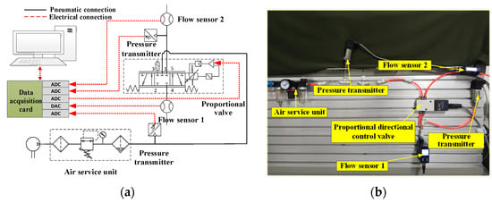
Figure 10.
Tests of the pneumatic circuit of the flow coefficient of the proportional valve: (a) schematic; (b) experimental test platform.
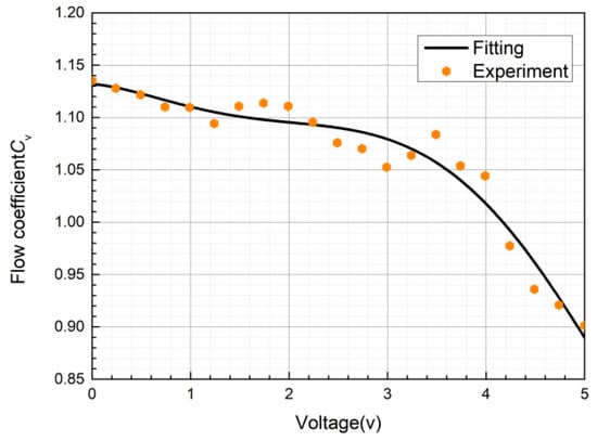
Figure 11.
Graph of flow coefficients and control voltages.
As shown in Figure 11, with the increase in the valve control voltage, the flow coefficient will gradually become smaller, indicating that the flow capacity of the gas through the valve port is getting smaller and smaller, and the control voltage range of the proportional directional control valve is 0–10 V. When , the valve core moves to the left. When , the spool moves to the right. The relationship between the control voltage and the valve spool displacement is shown in the following equation:
The mathematical relationship between the proportional valve spool displacement and the flow coefficient fitted by polynomial is:
4. Establishment of Differential Pressure Equations
Since the gases in Chambers A and B are regarded as ideal, the differential equation of state of the ideal gas results in a differential equation of pressure [22], which simplifies to:
In the formula, the volume of the two chambers of the cylinder is:
where is the initial volume of Chamber A, is the initial volume of Chamber B and the area of the piston.
5. Establishment of Kinetic Equations
5.1. Measurement of Stribeck Friction Model Parameters
The Stribeck friction model is also known as an exponential model [23]. In 1902, Stribeck found that the change in friction of an object moving at low speed shows a negative damping characteristic; that is, the friction will decrease with the increasing speed of the object. This is mainly because when an object is moving at low speed, the effective contact surface of the object is not in a state of sufficient lubrication. As the speed of the object gradually increases, the degree of lubrication of the object will also gradually increase. Therefore, the friction force will decrease. When the object is moving rapidly, the contact surface of the object is in a complete lubrication state, and the viscosity friction plays a dominant role and increases with the increasing speed. As shown in Figure 12, the relationship between friction and operating speed is described. Its friction model is as follows:
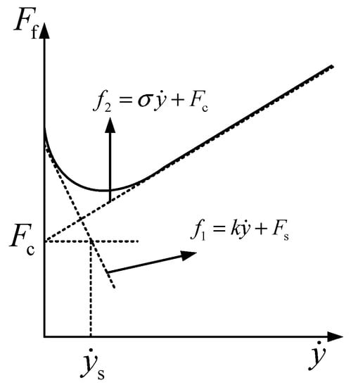
Figure 12.
Stribeck friction model graph.
When , the friction is:
When , the friction is:
where is a small positive constant, is the maximum static friction force, is the driving force of the piston, is the Coulomb friction force, is the angular velocity of the actuator, is Stribeck speed and is the viscous friction coefficient.
The Stribeck friction model has four unknown parameters, , , , , that need to be measured. The method of measurement is obtained by constructing auxiliary lines in the Stribeck friction model graph. The Stribeck friction model graph describes the relationship between the running speed of the object and the friction. The cylinder in the process of operation and its operating speed test method are as follows:
The magnetically coupled rodless cylinder has always been accompanied by friction during the working process. When the cylinder moves in a straight line at a low and uniform speed, the piston in the cylinder is only driven by the pressure difference between the two ends of the cylinder. Thus, the size of the friction force can be calculated according to Newton’s second law:
According to Equation (28), when the cylinder moves in a slow and uniform linear motion, the friction force of the cylinder is equal to the pressure difference between the two ends of the piston. Therefore, as long as the pressure difference between the two chambers of the cylinder is tested, the friction force of the cylinder in a state of slow and uniform motion can be obtained. The speed of the cylinder at la ow and uniform speed can be controlled by adjusting the control voltage of the proportional directional control valve. The data of the cylinder running at different slow and uniform speeds and the corresponding friction force can be brought into MATLAB’s fitting toolbox for curve fitting, and the Stribeck friction models curve diagram can be obtained.
The method of construction of the auxiliary line is shown in Figure 12. The curve of the cylinder at rest can be approximated by its tangent line , and the intersection of the straight line and the friction axis is the maximum static friction force . The curve of the cylinder in the motion stage is approximated by its tangent line f2, and the slope of the straight line f2 is expressed as the size of the viscous friction coefficient . The intersection point between the straight line and the frictional force axis is expressed as the size of the Coulomb friction force . The straight line parallel to the -axis is made, and the horizontal coordinate of the intersection of the straight line and the straight line is the critical velocity of Stribeck .
During the experiment, the supply pressure of the air source is 0.5 MPa. The pressure difference between the two ends of the cylinder at different speeds (slow and uniform speed) is measured by adjusting the control voltage of the proportional directional control valve. Then, brought into Formula (28), the corresponding friction force can be obtained. The speed at which the cylinder is operated is obtained by guiding time by the displacement of the uniform linear motion. The forward and reverse motions of the cylinder when the control voltage is 5.24 V and 4.395 V are shown in Figure 13 and Figure 14. By bringing the experimental data of the speed and friction at a slow and uniform speed operation to MATLAB for fitting, the resulting Stribeck friction model curve can be obtained, as shown in Figure 15.
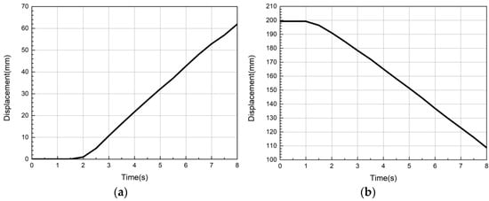
Figure 13.
Displacement graph: (a) forward motion; (b) reverse motion.
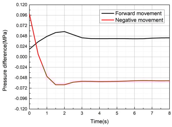
Figure 14.
Pressure difference graph.

Figure 15.
Friction fit graph.
From Figure 15, it can clearly be seen that the friction curve of the cylinder is significantly different during the forward and reverse motion, which is caused by the tilted installation of the slider in the lower part of the slider in the magnetically coupled rodless cylinder. Figure 16 shows the measurement process of the parameters of the Stribeck friction model during the forward and reverse motion of the cylinder, and the results are shown in Table 2.
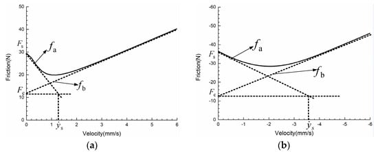
Figure 16.
Measurement diagram of frictional force parameters: (a) forward movement; (b) reverse movement.
Table 2.
Stribeck friction model parameter values.
5.2. Establishment of Kinetic Equations
According to Newton’s second law, the kinetic equation for a magnetically coupled rodless cylinder is:
Among them, the effective area of the piston is 0.00491 m2, which is the friction.
6. Validation of Nonlinear Models of the System
6.1. Validation of Inflation and Deflation of Fixed Chambers
The experimental platform for fixing the chamber inflation and deflation is shown in Figure 17. The experimental process is as follows: the supply pressure is set to 0.4 MPa. First the spool of the proportional directional control valve is adjusted to the end of the valve body, and then the control voltage is adjusted to 5.08 V. When the pressure of the two chambers of the cylinder is stabilized, the control voltage is adjusted to 4.4 V. At this time, Chamber A will be deflated, Chamber B will be inflated, and both will then slowly reach a stable state. The piston of the cylinder remains stationary throughout the experimental process [24]. In order to avoid the accident of the experiment, adjust the air supply pressures to 0.5 MPa and 0.6 MPa respectively, and repeat the above experimental process.
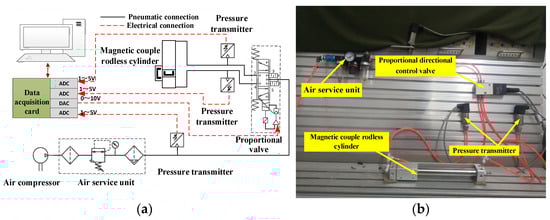
Figure 17.
Air-filling experiment diagram of fixed chamber: (a) experimental principle; (b) experimental test platform.
The simulated curve and the experimental results are shown in Figure 18, and the simulated curve is the same as the experimental curve, which can explain the correctness of the mathematical model. From the figure, we can find:
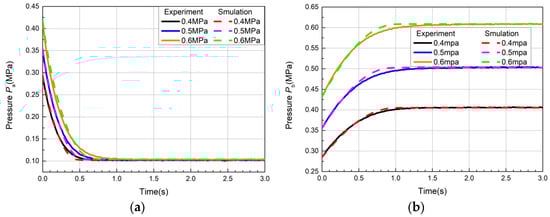
Figure 18.
Filling simulation and experimental diagram of fixed chamber: (a) Chamber A deflating; (b) Chamber B inflating.
- (1)
- With the increase in the supply pressure, when the pressure of the gas in the chamber reaches a stable value, the error between the experiment and the simulation will gradually increase. This is due to the fact that the greater the supply pressure, the leakage of the gas will gradually increase, meaning the experiment cannot be changed according to the ideal situation.
- (2)
- As the supply pressure increases, the initial pressure of the gas will gradually increase. This is because when the spool is located in the middle of the valve body, there is a gap between the spool and the valve sleeve, and the gas will enter the two chambers of the cylinder through the gap.
6.2. Positioning Experiment Verification of Nonlinear Model Systems
According to the pneumatic circuit shown in Figure 1, the nonlinear model is verified by PID-controlled positioning experiments. The air supply pressure is constant at 0.52 MPa, and given a step signal, the target position is 58. The results of the experiment and simulation are shown in Figure 19, because the cylinder inflation requires a certain reaction time during the experiment, and the simulation is carried out under ideal conditions, so the experimental reaction time will be slower than the simulation. However, the experiment is consistent with the trend of the simulation curve.
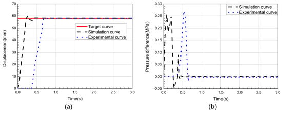
Figure 19.
Step signal position control graph: (a) displacement graph; (b) differential graph.
6.3. Trajectory Tracking Experimental Verification of Nonlinear Model Systems
Given a sinusoidal signal, trajectory tracking experimental verification based on PID control is performed. The frequency is set to 0.381 Hz, and the obtained experimental and simulation curves are shown in Figure 20. The trend of the experiment and the simulation curves are consistent, which proves the correctness of the simulation model.
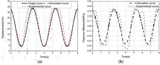
Figure 20.
Sine signal position control graph: (a) Displacement graph; (b) The differential graph.
The causes of experimental errors are:
- (1)
- The friction coefficient is variable during the experiment, and the fixed friction coefficient is considered when modeling and simulation, which will also produce a certain error;
- (2)
- There is a certain gas leakage in the gas circuit system and the cylinder;
- (3)
- The sensitivity of the sensor element is too small;
- (4)
- The instability of the gas supply pressure of the gas source.
7. Conclusions
In this paper, through the analysis and experimental test of the physical structure of the proportional control valve. the mathematical relationship between the valve port area and the control voltage of the proportional directional control valve, the mathematical relationship between the valve port flow coefficient and the valve core displacement is determined. Then, the mass flow equation of each valve port is established. Through the experimental test, the relevant parameters of the Stribeck friction model are determined, and the Stribeck friction model is applied to the kinematic equation. Finally, the gap between the valve core and the valve sleeve is proved by the inflation and deflation experiment of the fixed cavity, and the correctness of the mathematical model of the fixed cavity is verified. Through the positioning experiment and trajectory tracking experiment based on PID control, the results show that the trajectory of the simulation curve and the experimental curve is basically consistent, which verifies the correctness of the mathematical model of the position servo control system. The stability error between the positioning simulation curve and the experimental curve is less than 0.2 mm. The error between the trajectory tracking simulation curve and the experimental curve is less than 10 mm. This reflects the characteristics of the pneumatic position servo system.
Author Contributions
Conceptualization, Y.Z. and K.L.; Data curation, F.W.; Funding acquisition, Y.Z. and M.C.; Project administration, Y.Z.; Software, S.G.; Supervision, S.L. and B.L.; Writing—original draft, K.L.; Writing—review and editing, Y.Z. and K.L. All authors have read and agreed to the published version of the manuscript.
Funding
This work was funded by the Outstanding Young Scientists in Beijing (Grant No. BJJWZYJH01201910006021), Open Foundation of the State Key Laboratory of Fluid Power and Mechatronic Systems (Grant No. GZKF-202016), the Key Scientific and Technological Project of Henan Province (Grant No. 202102210081, 212102210050, 212102210006), Subproject of Strengthening Key Basic Research Projects in the Basic Plan of the Science and Technology Commission of the Military Commission (2019-JCJQ-ZD-120-13), and the Fundamental Research Funds for the Universities of Henan Province (Grant No. NSFRF200403).
Acknowledgments
The authors would like to thank Henan Polytechnic University, Beihang University and Zhejiang University for their support. The authors are sincerely grateful to the reviewers for their valuable review comments, which substantially improved the paper.
Conflicts of Interest
The authors declare no conflict of interest.
Nomenclature
| Mass flow rate of the gas in Chamber A or B (kg/s) | |
| Pressure of cylinder Chamber A or B (MPa) | |
| Temperature of cylinder Chamber A or B (K) | |
| Mass of the load (kg) | |
| Displacement of the cylinder (mm) | |
| Atmospheric pressure (MPa) | |
| Supply pressure (MPa) | |
| Mass flow rate of the gas flowing from Port 1 to Chamber A or B (kg/s) | |
| Mass flow rate of the gas flowing through Port 4 or 5 (kg/s) | |
| Mass flow rate of the gas flowing through Port 2 or 3 (kg/s) | |
| Length of the clearance (m) | |
| Inner diameter of the sleeve (m) | |
| Diameter of the spool shoulder (m) | |
| Effective area of the valve opening (mm2) | |
| Absolute pressure upstream of the valve body (MPa) | |
| Temperature upstream of the valve body (K) | |
| Volume flow through the valve port (L/min) | |
| Gas constant (J/(kg·K)) | |
| Critical pressure ratio | |
| Isentropic index | |
| Flow coefficient | |
| Initial length of the clearance (m) | |
| Spool displacement (m) | |
| Velocity of the gas micelles in the horizontal direction (m/s) | |
| Atmospheric density (kg/ m3) | |
| Viscosity coefficient of the gas (Pa·s) | |
| Mass flow rate of gas when the spool moves in the opposite direction (kg/s) | |
| Temperature under standard conditions (K) | |
| Control voltage (V) | |
| Initial volume of Chamber A or B (m3) | |
| Time (s) | |
| Thermodynamic energy change in a chamber (J) | |
| Velocity of the gas micelles in the horizontal direction (m/s) | |
| Initial volume of Chamber A or B (m3) | |
| Effective area of the actuator piston (m2) | |
| Coulomb friction force, friction and the maximum static friction force (N) | |
| Stribeck speed (mm/s) | |
| Viscous friction coefficient (N·s/mm) | |
| Speed of cylinder (mm/s) | |
| Positive constant |
References
- Wu, X. Modern Pneumatic Components and System; Chemical Industry Press: Beijing, China, 2015; Volume 1. [Google Scholar]
- Xie, Y.; Hao, C. Hydraulic and Pneumatic Technology; Fudan University Press: Shanghai, China, 2011; pp. 22–36. [Google Scholar]
- Wu, D. Greater development of pneumatic technology is expected. Hydraul. Pneum. Seals 2013, 9, 104–105. [Google Scholar]
- Yan, J.; Shi, P.; Zhang, X.B. Review of biomimetic mechanism, actuation, modeling and control in soft manipulators. J. Mech. Eng. 2018, 54, 1–14. [Google Scholar] [CrossRef]
- Li, X. The development for pneumatic drive. Mach. Build. Autom. 2003, 2, 5–7. [Google Scholar]
- Chen, Q. Thinking about the present and future development of china pneumatic industry suggestions to the 12th five-year development plan for pneumatic field. Hydraul. Pneum. Seals 2012, 32, 16–22. [Google Scholar]
- Luo, W.; Zhang, Q.; Huang, R.; Wang, S. Model of calculus of variation used for determination of sliding surface. J. Yangtze River Sci. Res. Inst. 2000, 3, 35–37. [Google Scholar]
- Liu, S.; Bobrow, J.E. An Analysis of a pneumatic servo system and its application to a computer-controlled robot. J. Dyn. Syst. Meas. Control 1988, 110, 228–235. [Google Scholar] [CrossRef]
- Rao, Z.; Bone, G.M. Non-linear Modeling and Control of Servo Pneumatic Actuators. IEEE Trans. Control. Syst. Technol. 2008, 16, 562–569. [Google Scholar]
- Lee, L.-W.; Li, I.-H. Wavelet-based adaptive sliding-mode control with H∞ tracking performance for pneumatic servo system position tracking control. IET Control. Theory Appl. 2012, 6, 1699–1714. [Google Scholar] [CrossRef]
- Blackburn, J.F.; Reethof, G.; Shearer, J.L. Fluid Power Control; Technology Press of M.I.T: Boston, MA, USA, 1966. [Google Scholar]
- Scavarda, S.; Kellal, A.; Richard, E. Linearised models for an electropneumatic cylinder servo valve system. In Proceedings of the Science and Engineering Education Lecture, Tokyo, Japan, 29 August 2013; pp. 306–307. [Google Scholar]
- Valdiero, A.C.; Ritter, C.S.; Rios, C.F.; Rafikov, M. Nonlinear mathematical modeling in pneumatic servo position applications. Math. Probl. Eng. 2011, 2011, 472903. [Google Scholar] [CrossRef]
- Bai, Y.; Li, X. Establishment of simulation model of pneumatic position servo system. Mach. Tool Hydraul. 2008, 7, 87–89, 128. [Google Scholar]
- Tao, G.; Mao, W.; W, X. Experimental study on mechanism modeling of pneumatic servo system. Hydraul. Pneum. Seals 1999, 5, 26–31. [Google Scholar]
- Wang, X. Modeling study of the PCM pneumatic servo system. Mach. Tool Hydraul. 1997, 4, 20–22. [Google Scholar]
- Bai, Y. Research on Pneumatic Rotation Position Servo Control Technology; Nanjing University of Science & Technology: Nanjing, China, 2006. [Google Scholar]
- Zhang, Y.; Li, K.; Wang, G.; Liu, J.; Cai, M. Nonlinear model establishment and experimental verification of a pneumatic rotary actuator position servo system. Energies 2019, 12, 1096. [Google Scholar] [CrossRef] [Green Version]
- Sanville, F.E. A new method of specifying the flow capacity of pneumatic fluid power valves. Hydraul. Pneum. Power 1971, 17, 120–126. [Google Scholar]
- Daugherty, R.L.; Ingersoll, A.C. Fluid Mechanics; McGraw Hill: New York, NY, USA, 1954. [Google Scholar]
- Wang, Y. Research Trajectory on Three-Axis Pneumatic Servo Space Control System; Harbin Institute of Technology: Harbin, China, 2008. [Google Scholar]
- Cai, M. Theory and Practice of Modern Pneumatic Technology Lecture 5: Characteristics of Cylinder Drive System. Hydraul. Pneum. Seals 2007, 6, 55–58. [Google Scholar]
- Yuan, D.; Liu, L.; Liu, H.; Wu, Z.; Wang, Z. Progress of Pre-sliding Friction Model. J. Syst. Simul. 2009, 4, 1142–1147. [Google Scholar]
- Zhang, Y.; Li, K.; Xu, M.; Liu, J.; Yue, H. Medical Grabbing Servo System with Friction Compensation Based on the Differential Evolution Algorithm. Chin. J. Mech. Eng. 2021, 34, 107. [Google Scholar] [CrossRef]
Publisher’s Note: MDPI stays neutral with regard to jurisdictional claims in published maps and institutional affiliations. |
© 2022 by the authors. Licensee MDPI, Basel, Switzerland. This article is an open access article distributed under the terms and conditions of the Creative Commons Attribution (CC BY) license (https://creativecommons.org/licenses/by/4.0/).